A point dislocation in a layered, transversely isotropic and self-gravitating Earth. Part I: analytical dislocation Love numbers

Zhou, J; Pan, E; Bevis, M

doi:10.1093/gji/ggz110

SUMMARY

In this paper, we derive analytical expressions for the dislocation Love numbers (DLNs) for a layered, spherical, transversely isotropic and self-gravitating Earth. This solution is based on the spherical system of vector functions (or the vector spherical harmonics) and a new propagating matrix method called the dual variable and position method. The DLNs can be obtained with high accuracy to an arbitrarily high degree, thereby allowing a wide range of applications based on high resolution earth models. Compared to the traditional numerical integration approach, the present analytical solution is at least 3 orders of magnitude faster. Our calculation also indicates that, compared to the isotropic PREM model, the effect of anisotropy is small, with a relative error about 5 per cent for DLN h¹² at degree n = 69 with source located at depth 100 km. We provide MATLAB code for computing the analytical DLNs in the supplementary materials section, along with a user manual.

Composition and structure of the mantle, Geomechanics, Theoretical seismology, Dynamics and mechanics of faulting, Mechanics, theory, and modelling

1 INTRODUCTION

Seismicity is an important geodynamic phenomenon. Earthquakes can cause great social and economic damage, but they also provide insights into plate motion, intraplate deformation, the mechanical structure of the earth and the behaviour of active fault systems. Earthquakes deform the Earth, producing redistributions of mass, stress and strain and causing measurable surface displacements as well as changes in the external gravity field.

Simulation of coseismic deformation was pioneered by Steketee (1958) who applied the theory of dislocations developed in solid-state physics to explain the strength of crystalline materials. This work was expanded by many geophysicists who examined numerous special classes of dislocation and fault movement, including vertical strike-slip faults, pure dip-slip faults and dislocations in Poisson solids. After a careful summary of previous work (e.g. Steketee 1958; Berry & Sales 1962; Maruyama 1964; Press 1965; Yamazaki 1978; Davis 1983), Okada (1985, 1992) presented a complete suite of closed analytical expressions for both surface and internal displacements, strains and tilts due to inclined shear and tensile faults in a homogeneous isotropic half-space. Both point dislocations and finite rectangular dislocations were considered. This analytical solution was extended to the finite triangular dislocation case by Meade (2007), and more recently by Nikkhoo & Walter (2015) where any possible pseudo singularity was completely removed. Okubo (1991) and Okubo (1992) examined analytically the potential and acceleration changes caused by point dislocations and by finite planar faults embedded in a homogeneous half-space. Analytical solutions were also derived for finite dislocations of polygonal shape in a transversely isotropic half-space (Pan et al.2014) and in a general anisotropic half-space (Pan et al.2015a).

The Earth is not homogeneous, and its material compositions and physical properties tend to change most rapidly in the vertical direction. Accordingly, layered half-space models are considerably more realistic than homogeneous half-space models. The elastic response to a dislocation embedded in a layered half-space is usually formulated using integral transforms, both for point dislocations (e.g. Singh 1970; Pan 1989) and finite dislocations (e.g. Fukahata & Matsu'ura 2005; Wang et al.2006).

The Earth is not flat, but approximately spherical in shape, so even a layered half-space solution is valid only in the near-field of an earthquake, say within ∼100 km. A more realistic earth model has to be spherical, layered and self-gravitating. Sun (1992) extended the dislocation theory from layered half-space to the layered spherical Earth and showed that the curvature effect is significant, especially for far-field results (Sun & Okubo 2002). This implies the necessity of using a spherical Earth. There exist some dislocation formulations and codes which incorporate layering and sphericity but ignore the impact of gravity (Pollitz 1992). This can also lead to significant prediction errors since the coupling between strain energy and gravitational potential energy needs to be considered (Gomez et al.2017). Invoking the dislocation problem in a layered spherical Earth with gravity significantly complicates its solution. For the special case of a homogeneous and elasto-gravitational sphere, an analytical solution exists (Love 1911; Gilbert & Backus 1968). Furthermore Love (1911) solved the force loading problem, which can be applied to find the corresponding dislocation solution by making use of Betti's reciprocity relation between the force solution and the dislocation solution (Pan 1991; Pan & Chen 2015). This reciprocity relation was further applied by Okubo (1993) to derive the relations between spherical coefficients in the surface-loading solution and the internal-dislocation solution. The reciprocity relation for the coefficients has been used to calculate coseismic displacement, geoid and strain changes (Sun 2003, 2004a, 2004b; Tang & Sun 2017), the deformation field due to surface rupture (Sun & Dong 2013), and more recently to simulate viscoelastic relaxation (Tang & Sun 2018).

We point out that besides the analytical solutions for a spherical Earth by Love (1911) and Gilbert & Backus (1968), various other analytical solutions have been derived and applied to problems in Earth science. Under the assumption of incompressibility, earth deformation by surface loading and by earthquakes were analytically solved, respectively, by Wu & Peltier (1982) for homogeneous sphere and Sabadini & Vermeersen (1997) for a layered sphere. Other analytical advances can be found in the recent monograph by Sabadini et al. (2016). On the other hand, for more realistic layered and spherical earth models, numerical methods, such as the Runge–Kutta integration, are normally utilized. This numerical method can be computationally expensive, even with the use of the reciprocity relation of Okubo (1993), when simulating the post-seismic transient deformation driven by viscoelastic relaxation (Wang 1999; Tanaka et al.2006).

Pan et al. (2015b) derived the analytical loading Love numbers for a spherically symmetric non-rotating, elastic and transversely isotropic (SNRETI) Earth. This is achieved by assuming that the density is constant and gravity varies linearly with radius in any layer within the Earth's core, while density is inversely proportional to radius and gravity is constant in any layer within the Earth's mantle. The isotropic (ISO) and transversely isotropic (TI) PREM models of Pan et al. (2015b) nearly overlap with the real earth PREM (Dziewonski & Anderson 1981). For instance, with only 56 mantle layers and 26 core layers, the difference of the material properties (including density and gravity) between the real PREM model and the ISO and TI PREM is less than l per cent in the entire core and less than 0.6 per cent in the entire mantle. Furthermore, one can easily further increase the accuracy in the discretized model by adding more layers. Chen et al. (2018) used this analytical solution and applied the stiffness matrix method to stably compute load Love numbers to an arbitrarily high degree. However, this analytical method has not been applied to the problem of internal dislocations. This motivates the present study.

Simulations of co- and post-seismic deformation are important to our understanding of Earth's mechanical properties, structure and behaviour. For instance, solutions obtained can be used to interpret ground- and space-based observations (Imanishi et al.2004; Sun & Okubo 2004; Heki & Matsuo 2010); to study earthquake-induced changes in Earth's rotation and polar motion (Chao & Gross 1987; Gross & Chao 2006; Zhou et al.2013, 2014; Cambiotti et al.2016), changes in its gravity field (Han et al.2006), and changes in reference frames (Zhou et al.2015, 2016), sea level variation (Melini et al.2010), as well as changes in Earth's volume (Xu & Sun 2014) and gravitational potential energy (Xu & Chao 2017; Zhou et al.2017). Therefore, an analytical solution for the dislocation Love numbers (DLNs) would greatly reduce the computational cost involved in calculating the DLNs and the associated Green's functions, for any given earth model. This desire also motivates the present study.

In this paper (Paper 1) we derive, for the first time, the analytical solutions for the DLNs within a layered, spherical and self-gravitating Earth. Some rocks exhibit transverse isotropy and the effect of this special and relatively simple class of anisotropy is sometimes significant (Pan et al.2014; Lynner et al.2018). Furthermore, the effective anisotropy could exist due to imbalanced tectonic stress and strain fields (Cambiotti et al.2014), and viscoelastic anisotropy could be large in mantle materials (Hansen et al.2012). As such, we further allow for the possibility of transverse isotropy in our earth model, though the user needs not to invoke it. We recognize that invoking transverse isotropy typically makes only minor changes to deformation solutions. However since it is relatively easy to incorporate transverse isotropy into the earth model, we do so to allow the user the freedom to invoke it whenever necessary.

We consider an internal point dislocation within the SNRETI Earth, which is also called a concentrated or infinitesimal dislocation, where the dislocation has a unit area, a given surface-normal direction and a 3-D Burgers’ vector. This paper is organized as follows: we first briefly describe the theory on how to analytically compute elastic DLNs in Section 2. Section 3 presents the source function expressions of a point dislocation by making use of the equivalent body-force method. Section 4 defines the DLNs for the four fundamental dislocations and the corresponding expressions of the Green's functions (to be used in Paper 2). Section 5 derives the Green's functions of an arbitrary dislocation from the results for the four fundamental dislocations. Section 6 verifies the accuracy and efficiency of our approach for calculating the DLNs. Conclusions are drawn in Section 7. Additionally, Appendix A presents the spherical system of vector functions or vector spherical harmonics. Appendix B discusses the specific cases of degrees n = 0 and 1. Appendix C lists the source functions of the four fundamental types of point dislocations, for both a TI and and ISO Earth. Appendix D provides the Green's function expressions for the displacements, gravity and geoid changes, as well as gravity disturbance at a given field point, induced by an arbitrary point dislocation.

2 THEORETICAL BASIS OF THE ANALYTICAL SOLUTIONS

The theory we use to obtain analytical solutions is briefly described below. The solutions are governed by the following first-order differential equations in terms of the spherical system of vector functions (i.e. Farrell 1972; Takeuchi & Saito 1972; see also Appendix A for easy reference).

\begin{eqnarray*} \frac{{{\rm{d}}{{\boldsymbol{Y}}^s}}}{{{\rm{d}}r}} = [{{\boldsymbol{B}}^s}{\rm{\ }}\left( {r,\rho ,g,{c_{ij}}} \right)]{{\boldsymbol{Y}}^s} \end{eqnarray*}

(1)

for spheroidal deformation (with superscript s), and

\begin{eqnarray*} \frac{{{\rm{d}}{{\boldsymbol{Y}}^t}}}{{{\rm{d}}r}} = [{{\boldsymbol{B}}^t}{\rm{\ }}\left( {r,{c_{ij}}} \right)]{{\boldsymbol{Y}}^t} \end{eqnarray*}

(2)

for toroidal deformation (with superscript t), where Y^s = [U_L, U_M, Φ, T_L, T_M, Q]^T and Y^t = [U_N, T_N]^T; the superscript T means transpose; the six (coefficient) components for spheroidal deformation refer to vertical displacement, horizontal displacement, potential change, vertical traction, horizontal traction and gravity flux, respectively; the two components for toroidal deformation are the horizontal displacement and horizontal traction, respectively; the two matrices [B^s] and [B^t] are functions of the radius r, density ρ, gravity g, and the elastic stiffness c_ij (in the Voigt notation). For the transversely isotropic medium, there are five independent components, which are also called elastic moduli.

While the analytical solutions based on the Gilbert–Backus formulation can be extended to the layered spherical Earth, such an approximation is unsatisfactory at low harmonic degrees and if the contribution of the internal buoyancy modes cannot be neglected (Cambiotti et al.2009). On the other hand, by looking closely at the data and curves in PREM model and considering further the possibility of an analytical solution, Pan et al. (2015b) came up perhaps the best and yet more realistic earth model which can be solved analytically. In this spherical and radially heterogeneous earth model made of multiple layers, the density is constant and gravity varies linearly with radius in each core layer, whilst the density variation is inversely linear with the radius and gravity is constant in each mantle layer. With only 56 mantle layers and 26 core layers, the material properties in the entire radial direction of Earth (in both core and mantle) overlap with the original PREM model (Dziewonski & Anderson 1981). In any jth layer bounded by r_j_-1 < r < r_j of the PREM model (Pan et al.2015b), by introducing the exponential variable substitution of r = r_j_-1e^ξ, eqs (1) and (2) can be transformed each into a linear system of first-order differential equations with constant coefficients, as

\begin{eqnarray*} \frac{{{\rm{d}}{{\boldsymbol{X}}^s}}}{{{\rm{d}}\xi }} = \left[ {{{\boldsymbol{C}}^s}} \right]{{\boldsymbol{X}}^s} \end{eqnarray*}

(3)

and

\begin{eqnarray*} \frac{{{\rm{d}}{{\boldsymbol{X}}^t}}}{{{\rm{d}}\xi }} = \left[ {{{\boldsymbol{C}}^t}} \right]{{\boldsymbol{X}}^t}, \end{eqnarray*}

(4)

respectively, where X^s = [U_L, U_M, Φ, rT_L, rT_M, rQ]^T, X^t = [U_N, rT_N]^T. Notice that matrices [C^s] and [C^t] in eqs (3) and (4) are now constants, independent of radius r if in each layer (when its thickness is relatively small) the five elastic moduli are constants. Consequently, eqs (3) and (4) both have analytical solutions which can be solved, for example via the propagator matrix method (e.g. Pan et al.2015b; Sabadini et al.2016).

The dislocation problem differs from the surface load problem in two ways: (1) there are discontinuities across or equivalent body forces at the source level, and hence there are inhomogeneous Dirac functions on the right-hand side of eqs (3) and (4), and (2) the boundary conditions are ‘traction’ free on the Earth's surface. Takeuchi & Saito (1972) showed that it was not necessary to directly solve the inhomogeneous differential equations, but instead, to solve twice the homogeneous differential equations. First, three general solutions with three unknown coefficients are obtained by setting three independent initial values in the Earth's centre. Then a particular solution is derived by integrating from the source to the Earth's surface with initial values being the given discontinuities of the source. Finally, the sum of the general and particular solutions must satisfy the traction-free boundary conditions on the surface, which determines the three unknown coefficients. In this paper, however, we introduce a novel and more efficient approach.

Although the solution on the Earth's surface can be analytically obtained by the propagator matrix method (e.g. Pan et al.2015b), numerical difficulties are introduced by round-off and propagating errors. The direct propagator matrix method in Pan et al. (2015b) was unable to provide correct results for higher harmonic degrees, say n > 6000. To overcome this problem, Chen et al. (2018) applied the stiffness matrix method to obtain stable results for arbitrary harmonic degree. In this paper, we employ yet another new method, called dual variable and position (DVP) method (e.g. Liu et al.2018), to propagate the solution from the Earth's centre to the surface. This method was developed and advanced from the well-known precise integration technique (e.g. Zhong et al.2004; Ai & Cheng 2014), and it has been shown to be very accurate and extremely powerful (e.g. Pan et al.2018). The main relations of the DVP method are described below, using the spheroidal case as an example.

The propagator matrix in each layer can be represented by an exponential matrix as

\begin{eqnarray*} [{e^{{{\boldsymbol{C}}^s}\xi }}] = [{\boldsymbol{P}}{\boldsymbol {\Lambda} }{{\boldsymbol{P}}^{ - 1}}] \end{eqnarray*}

(5)

in which superscript "−1" means matrix inverse; the exponentials of the eigenvalues of [C^s] form the diagonal matrix [Λ] and the corresponding eigenvectors of [C^s] form matrix [P]. It is straightforward that eq. (5) forms the basic solution of eq. (3). It should be noted that [PΛ] is also a basic solution of eq. (3). Furthermore, of all the eigenvalues, in general, half have positive real parts and the other half have negative real parts. Therefore, we can rearrange the basic solution eq. (5) to form the general solution of eq. (3) as

\begin{eqnarray*} {\boldsymbol{X}} = \left[ {\begin{array}{@{}*{2}{c}@{}} {{{\boldsymbol{A}}_1}}&{{{\boldsymbol{A}}_2}}\\ {{{\boldsymbol{B}}_1}}&{{{\boldsymbol{B}}_2}} \end{array}} \right]\ \left[ {\begin{array}{@{}*{2}{c}@{}} {\left\langle {{{\boldsymbol{s}}_1}\xi } \right\rangle }&0\\ 0&{\left\langle {{{\boldsymbol{s}}_2}\xi } \right\rangle } \end{array}} \right]\left[ {\begin{array}{@{}*{1}{c}@{}} {{{\boldsymbol{\kappa }}_1}}\\ {{{\boldsymbol{\kappa }}_2}} \end{array}} \right] \end{eqnarray*}

(6)

where the eigenvectors and eigenvalues are rearranged correspondingly, and

\begin{eqnarray*} \left\langle {{{\boldsymbol{s}}_1}\xi } \right\rangle = \left[ {\begin{array}{@{}*{3}{c}@{}} {{e^{\lambda _1^ + \xi }}}&0&0\\ 0&{{e^{\lambda _2^ + \xi }}}&0\\ 0&0&{{e^{\lambda _3^ + \xi }}} \end{array}} \right]\ ,\left\langle {{{\boldsymbol{s}}_2}\xi } \right\rangle = \left[ {\begin{array}{@{}*{3}{c}@{}} {{e^{\lambda _1^ - \xi }}}&0&0\\ 0&{{e^{\lambda _2^ - \xi }}}&0\\ 0&0&{{e^{\lambda _3^ - \xi }}} \end{array}} \right] \end{eqnarray*}

(7)

are two diagonal matrices being composed of exponential eigenvalues; s₁ and s₂ contain eigenvalues (λ_i; for i = 1 to 3) with positive and negative real parts, respectively; κ₁ and κ₂ are two unknown vectors to be determined by boundary/interface conditions. As a result, in jth layer (with 0 ≤ ξ≤ ξ_j), the solution can be expressed as

\begin{eqnarray*} {{\boldsymbol{X}}_j} = \left[ {\begin{array}{@{}*{2}{c}@{}} {{{\boldsymbol{A}}_1}}&{{{\boldsymbol{A}}_2}}\\ {{{\boldsymbol{B}}_1}}&{{{\boldsymbol{B}}_2}} \end{array}} \right]\ \left[ {\begin{array}{@{}*{2}{c}@{}} {\left\langle {{{\boldsymbol{s}}_1}(\xi - {\xi _j}} \right\rangle }&0\\ 0&{\left\langle {{{\boldsymbol{s}}_2}} \right\rangle } \end{array}} \right]\left[ {\begin{array}{@{}*{1}{c}@{}} {{{\boldsymbol{\kappa }}_1}}\\ {{{\boldsymbol{\kappa }}_2}} \end{array}} \right] \end{eqnarray*}

(8)

in which some constants are correspondingly combined into the components of the unknown vectors κ₁ and κ₂, which are to be determined.

Denoting U = [U_L, U_M, Φ]^Tand T = [T_L, T_M, Q]^T, and applying eq. (8) to the upper (ξ = ξ_j, denoted by superscript u) and lower (ξ = 0, denoted by superscript l) interfaces of the jth layer, we have

\begin{eqnarray*} \left[ {\begin{array}{@{}*{1}{c}@{}} {{\boldsymbol{U}}_j^u}\\ {{r_j}{\boldsymbol{T}}_j^u} \end{array}} \right] = \left[ {\begin{array}{@{}*{2}{c}@{}} {{{\boldsymbol{A}}_1}}&{{{\boldsymbol{A}}_2}}\\ {{{\boldsymbol{B}}_1}}&{{{\boldsymbol{B}}_2}} \end{array}} \right]\ \left[ {\begin{array}{@{}*{2}{c}@{}} {\boldsymbol{I}}&0\\ 0&{\left\langle {{{\boldsymbol{s}}_2}{\xi _j}} \right\rangle } \end{array}} \right]\left[ {\begin{array}{@{}*{1}{c}@{}} {{{\boldsymbol{\kappa }}_1}}\\ {{{\boldsymbol{\kappa }}_2}} \end{array}} \right];\quad \left[ {\begin{array}{@{}*{1}{c}@{}} {{\boldsymbol{U}}_j^l}\\ {{r_{j-1}}{\boldsymbol{T}}_j^l} \end{array}} \right] = \left[ {\begin{array}{@{}*{2}{c}@{}} {{{\boldsymbol{A}}_1}}&{{{\boldsymbol{A}}_2}}\\ {{{\boldsymbol{B}}_1}}&{{{\boldsymbol{B}}_2}} \end{array}} \right]\ \left[ {\begin{array}{@{}*{2}{c}@{}} {\left\langle { - {{\boldsymbol{s}}_1}{\xi _j}} \right\rangle }&0\\ 0&{\boldsymbol{I}} \end{array}} \right]\left[ {\begin{array}{@{}*{1}{c}@{}} {{{\boldsymbol{\kappa }}_1}}\\ {{{\boldsymbol{\kappa }}_2}} \end{array}} \right] \end{eqnarray*}

(9)

where [I] is the identity matrix of size 3 × 3.

Eliminating the unknown vectors κ₁ and κ₂ from eq. (9), we arrive at

\begin{eqnarray*} \left[ {\begin{array}{@{}*{1}{c}@{}} {{\boldsymbol{U}}_j^l}\\ {{r_j}{\boldsymbol{T}}_j^u} \end{array}} \right] = \left[ {\begin{array}{@{}*{2}{c}@{}} {{\boldsymbol{S}}_{11}^j}&{{\boldsymbol{S}}_{12}^j}\\ {{\boldsymbol{S}}_{21}^j}&{{\boldsymbol{S}}_{22}^j} \end{array}} \right]\ \left[ {\begin{array}{@{}*{1}{c}@{}} {{\boldsymbol{U}}_j^u}\\ {{r_{j-1}}{\boldsymbol{T}}_j^l} \end{array}} \right], \end{eqnarray*}

(10)

where

\begin{eqnarray*} \left[ {{{\boldsymbol{S}}^j}} \right] = \left[ {\begin{array}{@{}*{2}{c}@{}} {{\boldsymbol{S}}_{11}^j}&{{\boldsymbol{S}}_{12}^j}\\ {{\boldsymbol{S}}_{21}^j}&{{\boldsymbol{S}}_{22}^j} \end{array}} \right]{\rm{\ }} = \left[ {\begin{array}{@{}*{2}{c}@{}} {{{\boldsymbol{A}}_1}\left\langle { - {{\boldsymbol{s}}_1}{\xi _j}} \right\rangle }&{{{\boldsymbol{A}}_2}}\\ {{{\boldsymbol{B}}_1}}&{{{\boldsymbol{B}}_2}\left\langle {{{\boldsymbol{s}}_2}{\xi _j}} \right\rangle } \end{array}} \right]\ {\left[ {\begin{array}{@{}*{2}{c}@{}} {{{\boldsymbol{A}}_1}}&{{{\boldsymbol{A}}_2}\left\langle {{{\boldsymbol{s}}_2}{\xi _j}} \right\rangle }\\ {{{\boldsymbol{B}}_1}\left\langle { - {{\boldsymbol{s}}_1}{\xi _j}} \right\rangle }&{{{\boldsymbol{B}}_2}} \end{array}} \right]^{ - 1}}. \end{eqnarray*}

(11)

We emphasize that since the real parts of vector s₁ are all positive and those of s₂ are all negative, only exponentials with negative real parts are involved in eq. (11), which guarantees the computation stability. We further point out that the layer matrix (10) introduced in this paper is different from both the traditional propagator matrix (Pan et al.2015b) and the stiffness matrix (Chen et al.2018). It is this special ordering which makes the DVP method unique.

Similarly, we have, for (j + 1)th layer,

\begin{eqnarray*} \left[ {\begin{array}{@{}*{1}{c}@{}} {{\boldsymbol{U}}_{j + 1}^l}\\ {{r_{j + 1}}{\boldsymbol{T}}_{j + 1}^u} \end{array}} \right] = \left[ {\begin{array}{@{}*{2}{c}@{}} {{\boldsymbol{S}}_{11}^{j + 1}}&{{\boldsymbol{S}}_{12}^{j + 1}}\\ {{\boldsymbol{S}}_{21}^{j + 1}}&{{\boldsymbol{S}}_{22}^{j + 1}} \end{array}} \right]\ \left[ {\begin{array}{@{}*{1}{c}@{}} {{\boldsymbol{U}}_{j + 1}^u}\\ {{r_j}{\boldsymbol{T}}_{j + 1}^l} \end{array}} \right]. \end{eqnarray*}

(12)

Noting that |${\boldsymbol{U}}_j^u = {\boldsymbol{U}}_{j + 1}^l{\boldsymbol{\ }},{\boldsymbol{\ \ T}}_j^u = {\boldsymbol{T}}_{j + 1}^l{\boldsymbol{\ }}$| due to the continuity conditions on their common interface and further combining eqs (10) and (12), we arrive at

\begin{eqnarray*} \left[ {\begin{array}{@{}*{1}{c}@{}} {{\boldsymbol{U}}_j^l}\\ {{r_{j + 1}}{\boldsymbol{T}}_{j + 1}^u} \end{array}} \right] = \left[ {\begin{array}{@{}*{2}{c}@{}} {{\boldsymbol{S}}_{11}^{j:j + 1}}&{{\boldsymbol{S}}_{12}^{j:j + 1}}\\ {{\boldsymbol{S}}_{21}^{j:j + 1}}&{{\boldsymbol{S}}_{22}^{j:j + 1}} \end{array}} \right]\ \left[ {\begin{array}{@{}*{1}{c}@{}} {{\boldsymbol{U}}_{j + 1}^u}\\ {{r_{j-1}}{\boldsymbol{T}}_j^l} \end{array}} \right], \end{eqnarray*}

(13)

where the involved submatrices are defined as

\begin{eqnarray*} \left. {\begin{array}{@{}*{1}{c}@{}} {[{\boldsymbol{S}}_{11}^{j:j + 1}]{\rm{\ }} = \left[ {{\boldsymbol{S}}_{11}^j{\boldsymbol{S}}_{11}^{j + 1} + {\boldsymbol{S}}_{11}^j{\boldsymbol{S}}_{12}^{j + 1}{{\left\{ {{\boldsymbol{I}} - {\boldsymbol{S}}_{21}^j{\boldsymbol{S}}_{12}^{j + 1}} \right\}}^{ - 1}}{\boldsymbol{S}}_{21}^j{\boldsymbol{S}}_{11}^{j + 1}} \right]}\\ {[{\boldsymbol{S}}_{12}^{j:j + 1}]{\rm{\ }} = \left[ {{\boldsymbol{S}}_{11}^j{\boldsymbol{S}}_{12}^{j + 1}{{\left\{ {{\boldsymbol{I}} - {\boldsymbol{S}}_{21}^j{\boldsymbol{S}}_{12}^{j + 1}} \right\}}^{ - 1}}{\boldsymbol{S}}_{22}^j + {\boldsymbol{S}}_{12}^j} \right]}\\ {\left[ {{\boldsymbol{S}}_{21}^{j:j + 1}} \right]{\rm{\ }} = {\rm{\ }}\left[ {{\boldsymbol{\ S}}_{21}^{j + 1} + {\boldsymbol{S}}_{22}^{j + 1}{{\left\{ {{\boldsymbol{I}} - {\boldsymbol{S}}_{21}^j{\boldsymbol{S}}_{12}^{j + 1}} \right\}}^{ - 1}}{\boldsymbol{S}}_{21}^j{\boldsymbol{S}}_{11}^{j + 1}} \right]}\\ {\left[ {{\boldsymbol{S}}_{22}^{j:j + 1}} \right]{\rm{\ }} = \left[ {{\boldsymbol{S}}_{22}^{j + 1}{{\left\{ {{\boldsymbol{I}} - {\boldsymbol{S}}_{21}^j{\boldsymbol{S}}_{12}^{j + 1}} \right\}}^{ - 1}}{\boldsymbol{S}}_{22}^j} \right]} \end{array}} \right\} \end{eqnarray*}

(14)

eq. (13) is the important recursive relation in the DVP method. It relates the solutions in adjacent layers. Therefore, making use of eq. (13) repeatedly, we can propagate the solution from one layer to any other layer.

We now describe how to obtain solutions on the Earth's surface due to an internal dislocation. As Takeuchi & Saito (1972) pointed out, the inhomogeneous Dirac term can be transferred equivalently to the discontinuities across the source level at r_s as

\begin{eqnarray*} \left[ {\begin{array}{@{}*{1}{c}@{}} {{\boldsymbol{U}}\left( {r_s^ + } \right)}\\ {{r_s}{\boldsymbol{T}}\left( {r_s^ + } \right)} \end{array}} \right] = \left[ {\begin{array}{@{}*{1}{c}@{}} {{\boldsymbol{U}}\left( {r_s^ - } \right)}\\ {{r_s}{\boldsymbol{T}}\left( {r_s^ - } \right)} \end{array}} \right]{\boldsymbol{\ }} + \left[ {\begin{array}{@{}*{1}{c}@{}} {\Delta {\boldsymbol{U}}}\\ {{r_s}\Delta {\boldsymbol{T}}} \end{array}} \right], \end{eqnarray*}

(15)

where |$r_s^ + $| and |$r_s^ - $| mean the upper and lower sides of the source level r_s; the discontinuities |$\Delta {\boldsymbol{U}}$| and |$\Delta {\boldsymbol{T}}$| are defined in Section 3 and their final expressions are listed in Appendix C.

Unlike Pan et al. (2015b), where the entire core was assumed liquid, we assume more realistically here that there is a homogeneous inner solid core in the Earth. Therefore, three regular solutions at the interface of the inner solid core can be directly obtained according to Love (1911). They are represented by the spherical Bessel functions of first kind and power functions (Takeuchi & Saito 1972). These three solutions can then be connected to the lower interface of the (outer) liquid core so that they can be propagated to the core–mantle boundary. It is worth pointing out that our numerical results show that the inner solid core has only a very slight effect on the DLNs.

No matter if the outer liquid core is homogeneous or layered, and compressible or incompressible, we follow the same technique as in Pan et al. (2015b) to derive the solutions on the core–mantle boundary (r = r_c). For instance, for the layered and compressible outer liquid core, we have

\begin{eqnarray*} \left[ {\begin{array}{@{}*{1}{c}@{}} {{\boldsymbol{U}}\left( {{r_c}} \right)}\\ {{r_c}{\boldsymbol{T}}\left( {{r_c}} \right)} \end{array}} \right] = \left[ {\begin{array}{@{}*{1}{c}@{}} {{{\boldsymbol{M}}_1}}\\ {{{\boldsymbol{M}}_2}} \end{array}} \right]{\boldsymbol{\ c}} \end{eqnarray*}

(16)

in which (matrices [M₁] and [M₂] both being 3 × 3)

\begin{eqnarray*} \left[ {\begin{array}{@{}*{1}{c}@{}} {{{\boldsymbol{M}}_1}}\\ {{{\boldsymbol{M}}_2}} \end{array}} \right] = \left[ {\begin{array}{@{}*{3}{c}@{}} 0& \quad0& \quad1\\ 0& \quad1& \quad0\\ {\Phi \left( {{r_c}} \right)}& \quad0& \quad0\\ {{r_c}\rho \left( {{r_c}} \right)\Phi \left( {{r_c}} \right)}& \quad0& \quad{{r_c}\rho \left( {{r_c}} \right)g\left( {{r_c}} \right)}\\ 0& \quad0& \quad0\\ {{r_c}Y\left( {{r_c}} \right) + 4\pi G{r_c}\rho \left( {{r_c}} \right)\Phi \left( {{r_c}} \right)/g\left( {{r_c}} \right)}& \quad0& \quad{4\pi G{r_c}\rho \left( {{r_c}} \right)} \end{array}} \right] \end{eqnarray*}

(17a)

\begin{eqnarray*} {\boldsymbol{c}} = {\left[ {{c_1},{c_2},{c_3}} \right]^T}\ ;\ Y = Q - \frac{{4\pi G}}{g}{T_L}, \end{eqnarray*}

(17b)

where Q and T_L are the expansion coefficients on the core–mantle boundary (Pan et al.2015b; Chen et al.2018).

Applying eqs (13) and (14) from the core–mantle boundary (layer 1 in the mantle) to the source level r_s (on the lower side of the source level), we have

\begin{eqnarray*} \left[ {\begin{array}{@{}*{1}{c}@{}} {{\boldsymbol{U}}\left( {{r_c}} \right)}\\ {{r_s}{\boldsymbol{T}}\left( {r_s^ - } \right)} \end{array}} \right] = \left[ {\begin{array}{@{}*{2}{c}@{}} {{\boldsymbol{S}}_{11}^{1:k}}&{{\boldsymbol{S}}_{12}^{1:k}}\\ {{\boldsymbol{S}}_{21}^{1:k}}&{{\boldsymbol{S}}_{22}^{1:k}} \end{array}} \right]\ \left[ {\begin{array}{@{}*{1}{c}@{}} {{\boldsymbol{U}}\left( {r_s^ - } \right)}\\ {{r_c}{\boldsymbol{T}}\left( {{r_c}} \right)} \end{array}} \right] \end{eqnarray*}

(18)

in which we have assumed that the dislocation is located in the kth layer which has been subdivided into two sublayers.

Similarly from the source level (on the upper side of the source level) to the Earth's surface (r = a, of layer p), we have

\begin{eqnarray*} \left[ {\begin{array}{@{}*{1}{c}@{}} {{\boldsymbol{U}}\left( {r_s^ + } \right)}\\ {a{\boldsymbol{T}}\left( a \right)} \end{array}} \right] = \left[ {\begin{array}{@{}*{2}{c}@{}} {{\boldsymbol{S}}_{11}^{k:p}}&{{\boldsymbol{S}}_{12}^{k:p}}\\ {{\boldsymbol{S}}_{21}^{k:p}}&{{\boldsymbol{S}}_{22}^{k:p}} \end{array}} \right]\ \left[ {\begin{array}{@{}*{1}{c}@{}} {{\boldsymbol{U}}\left( a \right)}\\ {{r_s}{\boldsymbol{T}}\left( {r_s^ + } \right)} \end{array}} \right]. \end{eqnarray*}

(19)

Combining eqs (15), (16), (18) and (19), and further making use of the boundary condition T(a) = 0, we arrive at the following system of equations (after arranging all the given values to the right-hand side and all the unknowns to the left-hand side)

\begin{eqnarray*} \left[ {\begin{array}{@{}*{4}{c}@{}} {{\boldsymbol{S}}_{12}^{1:k}{{\boldsymbol{M}}_2} - {{\boldsymbol{M}}_1}}& \quad{\bf 0}& \quad{{\boldsymbol{S}}_{11}^{1:k}}& \quad{\bf 0}\\ {{\boldsymbol{S}}_{22}^{1:k}{{\boldsymbol{M}}_2}}& \quad{\bf 0}& \quad{{\boldsymbol{S}}_{21}^{1:k}}& \quad{ - {\boldsymbol{I}}}\\ {\bf 0}& \quad{{\boldsymbol{S}}_{11}^{k:p}}& \quad{ - {\boldsymbol{I}}}& \quad{{\boldsymbol{S}}_{12}^{k:p}}\\ {\bf 0}& \quad{{\boldsymbol{S}}_{21}^{k:p}}& \quad{\bf 0}& \quad{{\boldsymbol{S}}_{22}^{k:p}} \end{array}} \right]\ \left[ {\begin{array}{@{}*{1}{c}@{}} {\boldsymbol{c}}\\ {{\boldsymbol{U}}\left( a \right)}\\ {{\boldsymbol{U}}\left( {{r_{s - }}} \right)}\\ {{r_s}{\boldsymbol{T}}\left( {{r_{s - }}} \right)} \end{array}} \right] = \left[ {\begin{array}{@{}*{1}{c}@{}} {\bf 0}\\ {\bf 0}\\ {{\rm{\Delta }}{\boldsymbol{U}} - [{\boldsymbol{S}}_{12}^{k:p}]{r_s}{\rm{\Delta }}{\boldsymbol{T}}}\\ { - [{\boldsymbol{S}}_{22}^{k:p}]{r_s}{\rm{\Delta }}{\boldsymbol{T}}} \end{array}} \right], \end{eqnarray*}

(20)

where all the submatrices are 3 × 3. eq. (20) can be solved for all the unknowns involved. Particularly one can obtain the solution, U(a), on the Earth's surface. It is further noted that eq. (20) is valid only for degree n > 1. The solutions for degrees n = 0 and n = 1 are presented in Appendix B for easy reference.

Our propagating method, that is from the core–mantle boundary to the source level, and then from the source level to Earth's surface, is different from that of Takeuchi & Saito (1972) wherein the solution is propagated from core–mantle boundary to Earth's surface, and then from the source to Earth's surface. Numerical results show that our method results in the DLNs almost identical to those computed using the approach of Takeuchi & Saito (1972). Since our method requires less matrix propagation, that is propagating from the core–mantle boundary to source versus from the core–mantle boundary to Earth's surface, and furthermore it is analytical, it is more stable and computationally more efficient, particularly when n is large.

Furthermore, two novel techniques are introduced to suppress possible propagating errors. The first technique is the variable renormalization (by n). In other words, we define the following eight new independent variables

\begin{eqnarray*} {Y^s} = {\left[ {{U_L},r{T_L}/n,n{U_M},r{T_M},n\Phi ,rQ} \right]^T};\ \ {Y^t} = {\left[ {n{U_N},r{T_N}} \right]^T}\ . \end{eqnarray*}

(21)

In so doing, all the variables now have the same order of n, which makes the computation more stable when n is very large.

The second technique is to reverse the relations of eqs (18) and (19). In other words, we use the following new propagating relations

\begin{eqnarray*} \left[ {\begin{array}{@{}*{1}{c}@{}} {{\boldsymbol{U}}\left( {r_s^ - } \right)}\\ {{r_c}{\boldsymbol{T}}\left( {{r_c}} \right)} \end{array}} \right] = \left[ {\begin{array}{@{}*{2}{c}@{}} {{\boldsymbol{P}}_{11}^{1:k}}&{{\boldsymbol{P}}_{12}^{1:k}}\\ {{\boldsymbol{P}}_{21}^{1:k}}&{{\boldsymbol{P}}_{22}^{1:k}} \end{array}} \right]\ \left[ {\begin{array}{@{}*{1}{c}@{}} {{\boldsymbol{U}}\left( {{r_c}} \right)}\\ {{r_s}{\boldsymbol{T}}\left( {r_s^ - } \right)} \end{array}} \right] \equiv {\left[ {\begin{array}{@{}*{2}{c}@{}} {{\boldsymbol{S}}_{11}^{1:k}}&{{\boldsymbol{S}}_{12}^{1:k}}\\ {{\boldsymbol{S}}_{21}^{1:k}}&{{\boldsymbol{S}}_{22}^{1:k}} \end{array}} \right]^{ - 1}}\left[ {\begin{array}{@{}*{1}{c}@{}} {{\boldsymbol{U}}\left( {{r_c}} \right)}\\ {{r_s}{\boldsymbol{T}}\left( {r_s^ - } \right)} \end{array}} \right] \end{eqnarray*}

(22a)

\begin{eqnarray*} \left[ {\begin{array}{@{}*{1}{c}@{}} {{\boldsymbol{U}}\left( a \right)}\\ {{r_s}{\boldsymbol{T}}\left( {r_s^ + } \right)} \end{array}} \right] = \left[ {\begin{array}{@{}*{2}{c}@{}} {{\boldsymbol{P}}_{11}^{k:p}}&{{\boldsymbol{P}}_{12}^{k:p}}\\ {{\boldsymbol{P}}_{21}^{k:p}}&{{\boldsymbol{P}}_{22}^{k:p}} \end{array}} \right]\ \left[ {\begin{array}{@{}*{1}{c}@{}} {{\boldsymbol{U}}\left( {r_s^ + } \right)}\\ {a{\boldsymbol{T}}\left( a \right)} \end{array}} \right] \equiv {\left[ {\begin{array}{@{}*{2}{c}@{}} {{\boldsymbol{S}}_{11}^{k:p}}&{{\boldsymbol{S}}_{12}^{k:p}}\\ {{\boldsymbol{S}}_{21}^{k:p}}&{{\boldsymbol{S}}_{22}^{k:p}} \end{array}} \right]^{ - 1}}\left[ {\begin{array}{@{}*{1}{c}@{}} {{\boldsymbol{U}}\left( {r_s^ + } \right)}\\ {a{\boldsymbol{T}}\left( a \right)} \end{array}} \right]. \end{eqnarray*}

(22b)

In terms of these two new relations, eq. (20) is then replaced by

\begin{eqnarray*} \left[ {\begin{array}{@{}*{4}{c}@{}} { - {\boldsymbol{I}}}&{{\boldsymbol{P}}_{11}^{k:p}}&0&0\\ 0&{{\boldsymbol{P}}_{21}^{k:p}}&{ - {\boldsymbol{I}}}&0\\ 0&{ - {\boldsymbol{I}}}&{{\boldsymbol{P}}_{12}^{1:k}}&{{\boldsymbol{P}}_{11}^{1:k}{{\boldsymbol{M}}_1}}\\ 0&0&{{\boldsymbol{P}}_{22}^{1:k}}&{{\boldsymbol{P}}_{21}^{1:k}{{\boldsymbol{M}}_1} - {{\boldsymbol{M}}_2}} \end{array}} \right]\ \left[ {\begin{array}{@{}*{1}{c}@{}} {{\boldsymbol{U}}\left( a \right)}\\ {{\boldsymbol{U}}\left( {{r_{s - }}} \right)}\\ {{r_s}{\boldsymbol{T}}\left( {{r_{s - }}} \right)}\\ {\boldsymbol{c}} \end{array}} \right] = \left[ {\begin{array}{@{}*{1}{c}@{}} { - [{\boldsymbol{P}}_{11}^{k:p}]{\rm{\Delta }}{\boldsymbol{U}}}\\ { - \left[ {{\boldsymbol{P}}_{21}^{k:p}} \right]{\rm{\Delta }}{\boldsymbol{U}} + {r_s}{\rm{\Delta }}{\boldsymbol{T}}}\\ 0\\ 0 \end{array}} \right]. \end{eqnarray*}

(23)

It is noted that matrix [P] is the inverse of matrix [S] and that the source functions should be correspondingly changed according to eq. (21). Similar relations can be obtained for the corresponding toroidal deformation (by simply replacing any matrix or vector of dimension 3 in the spheroidal deformation by dimension 1 in the toroidal deformation).

3 SOURCE FUNCTIONS OF POINT DISLOCATIONS

Without loss of generality, we assume that there is a point dislocation of unit magnitude applied at (r,θ,ϕ) = (r_s,0,0) in layer k of the layered mantle. To find the discontinuity at the source level related to this concentrated dislocation, we rely on the equivalent body-force expression of a general dislocation over the internal area Σ (Aki & Richards 1980)

\begin{eqnarray*} \ {f_p} = - \iint {{c_{ijpq}}{\rm{\Delta }}u{v_i}{n_j}}\frac{{\partial \delta \left( {{\boldsymbol{r}} - {{\boldsymbol{r}}_s}} \right)}}{{{H_q}\partial q}}{\rm{d}}\Sigma , \end{eqnarray*}

(24)

where c_ijkl is the 4th-order stiffness tensor, Δu the dislocation magnitude, v_i the dislocation component along i-direction (or the i-direction of the Burgers’ vector), n_j the j-component of the normal of the infinitesimal dislocation area d∑, H_q the Lamé constant of the spherical coordinates, and

\begin{eqnarray*} \delta \ \left( {{\boldsymbol{r}} - {{\boldsymbol{r}}_s}} \right) = \frac{{\delta \left( {r - {r_s}} \right)\delta \left( \theta \right)\delta \left( \phi \right)}}{{{r^2}{\rm{sin}}\theta }}. \end{eqnarray*}

(25)

It is noted that summation is implied for repeated indices in eq. (24).

If the dislocation is concentrated at r_s = (r_s,0,0) then eq. (24) is changed to

\begin{eqnarray*} \ {f_p} = - {\rm{\Delta }}ud\Sigma \left[ {{c_{ijpq}}{v_i}{n_j}\frac{{\partial \delta \left( {r - {r_s}} \right)\delta \left( \theta \right)\delta \left( \phi \right)/r^2\rm\sin\theta}}{{{H_q}\partial q}}} \right]. \end{eqnarray*}

(26)

Expanding the equivalent force in terms of the vector spherical harmonics, that is substituting eq. (26) into eq. (A8) in Appendix A, it can be shown that the expansion coefficients of the equivalent force can be separated into two parts as

\begin{eqnarray*} \left[ {\begin{array}{@{}*{1}{c}@{}} {{F_L}\left( {r,n,m} \right)}\\ {{F_M}\left( {r,n,m} \right)}\\ {{F_N}\left( {r,n,m} \right)} \end{array}} \right] = \left[ {\begin{array}{@{}*{1}{c}@{}} {F_L^\delta }\\ {F_M^\delta }\\ {F_N^\delta } \end{array}} \right]\ \frac{{\delta \left( {r - {r_s}} \right)}}{{{r^3}}} + \left[ {\begin{array}{@{}*{1}{c}@{}} {F_L^d}\\ {F_M^d}\\ {F_N^d} \end{array}} \right]\frac{{\partial \delta \left( {r - {r_s}} \right)}}{{{r^2}\partial r}}. \end{eqnarray*}

(27)

The first term on the right-hand side induces discontinuities in tractions only and the second term causes discontinuities in both tractions and displacements. Combining the discontinuities by both terms, the following source functions can be found (Takeuchi & Saito 1972; Kennett 1983).

\begin{eqnarray*} \left[ {\begin{array}{@{}*{1}{c}@{}} {{\rm{\Delta }}{{\boldsymbol{U}}^s}\left( {{r_s},\ n,\ m} \right)}\\ {{r_s}{\rm{\Delta }}{{\boldsymbol{T}}^s}\left( {{r_s},\ n,\ m} \right)} \end{array}} \right] = \left[ {\begin{array}{@{}*{1}{c}@{}} 0\\ 0\\ 0\\ {{r_s}F_L^\delta }\\ {{r_s}F_M^\delta }\\ 0 \end{array}} \right] + {{\boldsymbol{C}}^s}\left[ {\begin{array}{@{}*{1}{c}@{}} 0\\ 0\\ 0\\ {{r_s}F_L^d}\\ {{r_s}F_M^d}\\ 0 \end{array}} \right] \end{eqnarray*}

(28a)

for spheroidal deformation, and

\begin{eqnarray*} \left[ {\begin{array}{@{}*{1}{c}@{}} {{U_N}\left( {{r_s},\ n,\ m} \right)}\\ {{r_s}{T_N}\left( {{r_s},\ n,\ m} \right)} \end{array}} \right] = \left[ {\begin{array}{@{}*{1}{c}@{}} 0\\ {{r_s}F_N^\delta } \end{array}} \right] + {{\boldsymbol{C}}^t}\left[ {\begin{array}{@{}*{1}{c}@{}} 0\\ {{r_s}F_N^d} \end{array}} \right] \end{eqnarray*}

(28b)

for toroidal deformation.

The final discontinuities are listed in Appendix C for easy reference.

4 DLNS AND GREEN'S FUNCTIONS

With the solutions of the coefficients U_L, U_M and Φ on the Earth's surface, we can derive the DLNs. To simplify the computation, we remove the common factors which depend on the harmonic degree n and source depth r_s in eq. (C1) in Appendix C. These factors will be recovered in computing the Green's functions. The imaginary unit i is also processed similarly. In what follows, we define the DLNs and derive the corresponding Green's functions of the spheroidal and toroidal displacements (at a given radius r in the mantle) for the four fundamental dislocations (Ben-Menahem & Singh 1981; Sun & Okubo 1993).

The Burgers vector associated with a dislocation characterizes the relative motion of two points on opposite sides of the dislocation surface when the distance between these points is infinitesimally small. Let the Burger's vector be v and the normal to the dislocation surface be n. There are two unit normals for any flat surface: they have opposite signs and point in opposite directions. We choose n so that it defines (by pointing towards) the ‘positive’ side of the dislocation, allowing us to establish a sign convention for the Burgers vector v. We define v = (u₊ − u₋), where u₊ and u₋ are the displacement vectors on the positive and negative sides of the dislocation, respectively. We decompose both vectors, v and n, in a local, right-handed, Cartesian coordinate system with its origin at the centre of the dislocation, and its 1, 2 and 3 axes are the unit vectors e_θ, e_φ and e_r, respectively (Fig. 1). This axis system is also referred to as the SEU axis system since its axes point south, east and up. The Burger's vector v has components (v₁,v₂,v₃) or equivalently (v_s,v_e,v_u), and the normal vector has components (n₁,n₂,n₃) or equivalently (n_s,n_e,n_u). For an isotropic or transversely isotropic medium, it is possible to characterize a dislocation with any orientation and any Burgers vector as a linear combination of four elementary dislocations (Sun & Okubo 1993) in which the normal vector and the Burgers vector are both unit vectors aligned with the 1, 2 or 3 axes [e.g. see Ben-Menahem & Singh (1981) for a review of this and surrounding concepts].

Figure 1.

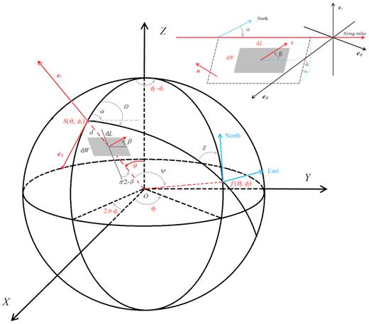
Geometric relations in spherical coordinates among both global and local orientation angles and distances. The source coordinate of the fault is at (r_s,θ_s,ϕ_s) and its epicentre is at s(a,θ_s,ϕ_s). The observation point or the field point is located on the surface at f(a,θ_f,ϕ _f). East is along e_ϕ, South along e_θ, up along e_r. The zoom-in fault parameters are: depth d = a − r_s, strike α, dip δ, slip β, length dL, width dW, slip vector ν, and fault normal n.

Open in new tab Download slide

Following Sun & Okubo (1993) we specify the standard dislocation modes with a double index i j in which i refers to the direction of the unit Burgers vector and j refers to the direction of the unit normal vector. Thus the ‘12″ mode means v = (1,0,0) and n = (0,1,0), so the fault normal points east, (i.e. it is a vertical fault that strikes north), and the unit Burger's vector points south, meaning that this is a vertical, right-lateral, strike-slip fault. This is one of the four standard modes of dislocation. Two of them are shear dislocations and the other two are tensile (i.e. dilatational or opening-mode) dislocations, as summarized in Table 1.

Table 1.

Open in new tab

The four standard dislocations: their unit Burgers vectors and unit normal vectors.

	Burgers (v₁,v₂,v₃)	Normal (n₁,n₂,n₃)
Mode index	(s, e, u)	(s, e, u)	Geological description: H = horizontal, V = vertical, SS = strike-slip, DS = dip-slip, T = tensile, RL = right lateral
12	(1,0,0)	(0,1,0)	V RL SS fault, strikes north, east wall moves south
32	(0,0,1)	(0,1,0)	V DS fault, strikes north, east wall moves up
22	(0,1,0)	(0,1,0)	V T fault, strikes north, east wall moves east (opening)
33	(0,0,1)	(0,0,1)	H T fault, upper wall moves up (opening)

	Burgers (v₁,v₂,v₃)	Normal (n₁,n₂,n₃)
Mode index	(s, e, u)	(s, e, u)	Geological description: H = horizontal, V = vertical, SS = strike-slip, DS = dip-slip, T = tensile, RL = right lateral
12	(1,0,0)	(0,1,0)	V RL SS fault, strikes north, east wall moves south
32	(0,0,1)	(0,1,0)	V DS fault, strikes north, east wall moves up
22	(0,1,0)	(0,1,0)	V T fault, strikes north, east wall moves east (opening)
33	(0,0,1)	(0,0,1)	H T fault, upper wall moves up (opening)

Table 1.

Open in new tab

The four standard dislocations: their unit Burgers vectors and unit normal vectors.

	Burgers (v₁,v₂,v₃)	Normal (n₁,n₂,n₃)
Mode index	(s, e, u)	(s, e, u)	Geological description: H = horizontal, V = vertical, SS = strike-slip, DS = dip-slip, T = tensile, RL = right lateral
12	(1,0,0)	(0,1,0)	V RL SS fault, strikes north, east wall moves south
32	(0,0,1)	(0,1,0)	V DS fault, strikes north, east wall moves up
22	(0,1,0)	(0,1,0)	V T fault, strikes north, east wall moves east (opening)
33	(0,0,1)	(0,0,1)	H T fault, upper wall moves up (opening)

	Burgers (v₁,v₂,v₃)	Normal (n₁,n₂,n₃)
Mode index	(s, e, u)	(s, e, u)	Geological description: H = horizontal, V = vertical, SS = strike-slip, DS = dip-slip, T = tensile, RL = right lateral
12	(1,0,0)	(0,1,0)	V RL SS fault, strikes north, east wall moves south
32	(0,0,1)	(0,1,0)	V DS fault, strikes north, east wall moves up
22	(0,1,0)	(0,1,0)	V T fault, strikes north, east wall moves east (opening)
33	(0,0,1)	(0,0,1)	H T fault, upper wall moves up (opening)

4.1 Vertical strike-slip (v₁ = 1, n₂ = 1) for m = ± 2 (denoted with superscript "12")

The DLNs at radius r are defined as

\begin{eqnarray*} \left. {\begin{array}{@{}*{1}{c}@{}} {h_n^{12}\ \left( r \right) = U_L^{12}\ \left( r \right)}\\ {l_n^{12}\ \left( r \right) = U_M^{12}\ \left( r \right)}\\ {k_n^{12}\ \left( r \right) = {\Phi ^{12}}\ \left( r \right)/{g_a}}\\ {l_n^{t,12}\ \left( r \right) = U_N^{12}\ \left( r \right)} \end{array}} \right\}, \end{eqnarray*}

(29)

where g_a is the gravity on the Earth's surface and |$U_L^{12},U_M^{12},U_N^{12},{\Phi ^{12}}$| are the expansion coefficients of the displacement and potential change at r due to the vertical strike-slip source at r = r_s

\begin{eqnarray*} \left. {\begin{array}{@{}*{1}{c}@{}} {\ {\rm{\Delta }}U_L^{12} = 0;{r_s}\ {\rm{\Delta }}T_L^{12} = 0;\ \ {\rm{\Delta }}U_M^{12} = 0}\\ {{r_s}\ {\rm{\Delta }}T_M^{12} = \pm \frac{{{c_{66}}}}{2},\ \ \ m = \pm 2}\\ {\ {\rm{\Delta }}U_N^{12} = 0}\\ {{r_s}\ {\rm{\Delta }}T_N^{12} = \frac{{{c_{66}}}}{2},\ \ \ m = \pm 2} \end{array}} \right\}. \end{eqnarray*}

(30)

Therefore the Green's functions of the spheroidal and toroidal displacements are as follows.

The vertical displacement on the Earth's surface is

\begin{eqnarray*} {\boldsymbol{u}}_L^{12}\ \left( {\theta ,} \right) &=& i\mathop \sum \nolimits_{n\ = \ 2}^\infty h_n^{12}\left( a \right){F^{12}}\left[ {{\boldsymbol{L}}\left( {\theta ,\phi ;n,2} \right) - {{\left( { - 1} \right)}^2}{{\boldsymbol{L}}^{\boldsymbol{*}}}\left( {\theta ,\phi ;n,2} \right)} \right] \nonumber \\ &=& - 2\mathop \sum \nolimits_{n\ = \ 2}^\infty h_n^{12}\left( a \right){F^{12}}\ {\rm{Im}}\left[ {S\left( {\theta ,\phi ;n,2} \right)} \right]{{\boldsymbol{e}}_r} , \end{eqnarray*}

(31)

where Im[S] means imaginary part of the spherical harmonic function S. Therefore

\begin{eqnarray*} {\boldsymbol{u}}_L^{12}\ \left( {\theta ,\phi } \right) = - 2\mathop \sum \nolimits_{n\ = \ 2}^\infty h_n^{12}\left( a \right){F^{12}}\bar{P}_n^2\left( {{\rm{cos}}\theta } \right){\rm{sin}}2\phi {{\boldsymbol{e}}_r} \end{eqnarray*}

(32)

through which, omitting the longitude dependence variable ϕ, we define the Green's function of the vertical displacement as

\begin{eqnarray*} \bar{u}_r^{12}\ \left( \theta \right) = - 2\mathop \sum \nolimits_{n\ = \ 2}^\infty h_n^{12}\left( a \right){F^{12}}\bar{P}_n^2\left( {{\rm{cos}}\theta } \right). \end{eqnarray*}

(33)

Similarly, the horizontal displacements are

\begin{eqnarray*} {\boldsymbol{u}}_M^{12}\ \left( {\theta ,\phi } \right) &=& i\mathop \sum \nolimits_{n\ = \ 2}^\infty l_n^{12}\left( a \right){F^{12}}\left[ {{\boldsymbol{M}}\left( {\theta ,\phi ;n,2} \right) - {{\left( { - 1} \right)}^2}{{\boldsymbol{M}}^{\boldsymbol{*}}}\left( {\theta ,\phi ;n,2} \right)} \right] \nonumber \\ &=& - 2\mathop \sum \nolimits_{n\ = \ 2}^\infty l_n^{12}\left( a \right){F^{12}}\left[ {{{\boldsymbol{e}}_\theta }\frac{{\partial \bar{P}_n^2\left( {{\rm{cos}}\theta } \right)}}{{\partial \theta }}{\rm{sin}}2\phi + {{\boldsymbol{e}}_\phi }\frac{{\bar{P}_n^2\left( {{\rm{cos}}\theta } \right)}}{{{\rm{sin}}\theta }}2{\rm{cos}}2\phi } \right] \end{eqnarray*}

(34a)

\begin{eqnarray*} {\boldsymbol{u}}_N^{12}\ \left( {\theta ,\phi } \right) &=& \mathop \sum \nolimits_{n = 2}^\infty l_n^{t,12}\left( a \right){F^{12}}\left[ {{\boldsymbol{N}}\left( {\theta ,\phi ;n,2} \right) + {{\left( { - 1} \right)}^2}{{\boldsymbol{N}}^{\boldsymbol{*}}}\left( {\theta ,\phi ;n,2} \right)} \right] \nonumber \\ &=& - 2\mathop \sum \nolimits_{n\ = \ 2}^\infty l_n^{t,12}\left( a \right){F^{12}}\left[ {{{\boldsymbol{e}}_\theta }\frac{{\bar{P}_n^2\left( {{\rm{cos}}\theta } \right)}}{{{\rm{sin}}\theta }}2{\rm{sin}}2\phi + {{\boldsymbol{e}}_\phi }\frac{{\partial \bar{P}_n^2\left( {{\rm{cos}}\theta } \right)}}{{\partial \theta }}{\rm{cos}}2\phi } \right] . \end{eqnarray*}

(34b)

Then the corresponding Green's functions of the spheroidal and toroidal horizontal displacements are defined as, by omitting their dependence on the longitude variable ϕ,

\begin{eqnarray*} \bar{u}_\theta ^{s,12}\ \left( \theta \right) = - 2\mathop \sum \nolimits_{n\ = \ 2}^\infty l_n^{12}\left( a \right){F^{12}}\frac{{\partial \bar{P}_n^2\left( {{\rm{cos}}\theta } \right)}}{{\partial \theta }} \end{eqnarray*}

(35a)

\begin{eqnarray*} \bar{u}_\phi ^{s,12}\left( \theta \right) = - 2\mathop \sum \nolimits_{n\ = \ 2}^\infty l_n^{12}\left( a \right){F^{12}}\frac{{\bar{P}_n^2\left( {{\rm{cos}}\theta } \right)}}{{{\rm{sin}}\theta }} \end{eqnarray*}

(35b)

\begin{eqnarray*} \bar{u}_\theta ^{t,12}\left( \theta \right) = - 2\mathop \sum \nolimits_{n\ = \ 2}^\infty l_n^{t,12}\left( a \right){F^{12}}\frac{{\bar{P}_n^2\left( {{\rm{cos}}\theta } \right)}}{{{\rm{sin}}\theta }} \end{eqnarray*}

(35c)

\begin{eqnarray*} \bar{u}_\phi ^{t,12}\ \left( \theta \right) = - 2\mathop \sum \nolimits_{n\ = \ 2}^\infty l_n^{t,12}\left( a \right){F^{12}}\frac{{\partial \bar{P}_n^2\left( {{\rm{cos}}\theta } \right)}}{{\partial \theta }}. \end{eqnarray*}

(35d)

In the above equations, the common factor is defined as

\begin{eqnarray*} {F^{12}}\ \left( {n,{r_s}} \right) = \frac{1}{{r_s^2}}\ \sqrt {\frac{{\left( {2n + 1} \right)\left( {n + 2} \right)\left( {n - 1} \right)}}{{4\pi n\left( {n + 1} \right)}}} . \end{eqnarray*}

(36)

4.2 Vertical dip-slip (v₃ = 1, n₂ = 1) for m = ± 1 (denoted with superscript "32")

The DLNs at radius r are defined as

\begin{eqnarray*} \left. {\begin{array}{@{}*{1}{c}@{}} {h_n^{32}\ \left( r \right) = U_L^{32}\ \left( r \right)}\\ {l_n^{32}\ \left( r \right) = U_M^{32}\ \left( r \right)}\\ {k_n^{32}\ \left( r \right) = {\Phi ^{32}}\ \left( r \right)/{g_a}}\\ {l_n^{t,32}\ \left( r \right) = U_N^{32}\ \left( r \right)} \end{array}} \right\} \end{eqnarray*}

(37)

where |$U_L^{32},\ U_M^{32},\ U_N^{32},{\Phi ^{32}}$| are the expansion coefficients of the displacement and potential change at r due to the vertical dip-slip source at r = r_s

\begin{eqnarray*} \left. {\begin{array}{@{}*{1}{c}@{}} {\ {\rm{\Delta }}U_L^{32} = 0;{r_s}\ {\rm{\Delta }}T_L^{32} = 0;{r_s}{\rm{\Delta }}T_M^{32}\ = 0}\\ {\ {\rm{\Delta }}U_M^{32} = - \frac{1}{2},\ \ \ m = \pm 1}\\ {\ {\rm{\Delta }}U_N^{32} = \mp \frac{1}{2},\ \ \ m = \ \pm 1}\\ {{r_s}\ {\rm{\Delta }}T_N^{32} = 0} \end{array}} \right\} \end{eqnarray*}

(38)

Similarly, the vertical displacement is

\begin{eqnarray*} {\boldsymbol{u}}_L^{32}\ \left( {\theta ,\phi } \right) &=& i\mathop \sum \nolimits_{n\ = \ 1}^\infty h_n^{32}\left( a \right){F^{32}}\left[ {{\boldsymbol{L}}\left( {\theta ,\phi ;n,1} \right) + {{\left( { - 1} \right)}^1}{{\boldsymbol{L}}^{\boldsymbol{*}}}\left( {\theta ,\phi ;n,1} \right)} \right] \nonumber \\ &=& - 2\mathop \sum \nolimits_{n\ = \ 2}^\infty h_n^{32}\left( a \right){F^{32}}\bar{P}_n^1\left( {{\rm{cos}}\theta } \right)\sin \phi {{\boldsymbol{e}}_r} \end{eqnarray*}

(39)

The Green's function is

\begin{eqnarray*} \bar{u}_r^{32}\ \left( \theta \right) = - 2\mathop \sum \nolimits_{n\ = \ 2}^\infty h_n^{32}\left( a \right){F^{32}}\bar{P}_n^1\left( {{\rm{cos}}\theta } \right) \end{eqnarray*}

(40)

The spheroidal and toroidal horizontal displacements are, respectively,

\begin{eqnarray*} {\boldsymbol{u}}_M^{32} \left( {\theta ,\phi } \right) &=& i\mathop \sum \nolimits_{n\ = \ 1}^\infty l_n^{32}\left( a \right){F^{32}}\left[ {{\boldsymbol{M}}\left( {\theta ,\phi ;n,1} \right) + {{\left( { - 1} \right)}^1}{{\boldsymbol{M}}^{\boldsymbol{*}}}\left( {\theta ,\phi ;n,1} \right)} \right] \nonumber \\ &=& - 2\mathop \sum \nolimits_{n\ = \ 1}^\infty l_n^{32}\left( a \right){F^{32}}\left[ {{{\boldsymbol{e}}_\theta }\frac{{\partial \bar{P}_n^1\left( {{\rm{cos}}\theta } \right)}}{{\partial \theta }}{\rm{sin}}\phi + {{\boldsymbol{e}}_\phi }\frac{{\bar{P}_n^1\left( {{\rm{cos}}\theta } \right)}}{{{\rm{sin}}\theta }}\cos \phi } \right] \end{eqnarray*}

(41a)

\begin{eqnarray*} {\boldsymbol{u}}_N^{32}\ \left( {\theta ,} \right) &=& \mathop \sum \nolimits_{n = 2}^\infty l_n^{t,32}\left( a \right){F^{32}}\left[ { - {\boldsymbol{N}}\left( {\theta ,\phi ;n,1} \right) + {{\left( { - 1} \right)}^1}{{\boldsymbol{N}}^{\boldsymbol{*}}}\left( {\theta ,\phi ;n,1} \right)} \right] \nonumber \\ &=& - 2\mathop \sum \nolimits_{n\ = \ 1}^\infty l_n^{t,32}\left( a \right){F^{32}}\left[ {{{\boldsymbol{e}}_\theta }\frac{{\partial \bar{P}_n^1\left( {{\rm{cos}}\theta } \right)}}{{\partial \theta }}\sin \phi + {{\boldsymbol{e}}_\phi }\frac{{\bar{P}_n^1\left( {{\rm{cos}}\theta } \right)}}{{{\rm{sin}}\theta }}\cos \phi } \right] \end{eqnarray*}

(41b)

Correspondingly, the Green's functions are defined as

\begin{eqnarray*} \bar{u}_\theta ^{s,32}\ \left( \theta \right) = - 2\mathop \sum \nolimits_{n\ = \ 2}^\infty l_n^{32}\left( a \right){F^{32}}\frac{{\partial \bar{P}_n^1\left( {{\rm{cos}}\theta } \right)}}{{\partial \theta }} \end{eqnarray*}

(42a)

\begin{eqnarray*} \bar{u}_\phi ^{s,32}\left( \theta \right) = - 2\mathop \sum \nolimits_{n = 2}^\infty l_n^{32}\left( a \right){F^{32}}\frac{{\bar{P}_n^1\left( {{\rm{cos}}\theta } \right)}}{{{\rm{sin}}\theta }} \end{eqnarray*}

(42b)

\begin{eqnarray*} \bar{u}_\theta ^{t,32}\ \left( \theta \right) = - 2\mathop \sum \nolimits_{n\ = \ 2}^\infty l_n^{t,32}\left( a \right){F^{32}}\frac{{\bar{P}_n^1\left( {{\rm{cos}}\theta } \right)}}{{{\rm{sin}}\theta }} \end{eqnarray*}

(42c)

\begin{eqnarray*} \bar{u}_\phi ^{t,32}\ \left( \theta \right) = - 2\mathop \sum \nolimits_{n\ = \ 2}^\infty l_n^{t,32}\left( a \right){F^{32}}\frac{{\partial \bar{P}_n^1\left( {{\rm{cos}}\theta } \right)}}{{\partial \theta }} \end{eqnarray*}

(42d)

where the common factor is defined as

\begin{eqnarray*} {F^{32}}\ \left( {n,{r_s}} \right) = \frac{1}{{r_s^2}}\ \sqrt {\frac{{2n + 1}}{{4\pi n\left( {n + 1} \right)}}} \end{eqnarray*}

(43)

4.3 Horizontal tensile fracture (v₂ = 1, n₂ = 1) for m = 0 and m = ± 2 (denoted with superscript "22")

This type of dislocation is special because both m = 0 and m = ± 2 contribute to the source functions, and needs to be discussed separately.

First for m = 0. The DLNs at radius r are defined as

\begin{eqnarray*} \left. {\begin{array}{@{}*{1}{c}@{}} {h_n^{22}\ \left( r \right) = U_L^{22}\ \left( r \right)}\\ {l_n^{22}\ \left( r \right) = U_M^{22}\ \left( r \right)}\\ {k_n^{22}\ \left( r \right) = {\Phi ^{22}}\ \left( r \right)/{g_a}}\\ {l_n^{t,22}\ \left( r \right) = U_N^{22}\ \left( r \right)} \end{array}} \right\} \end{eqnarray*}

(44)

where |$U_L^{22},U_M^{22},U_N^{22},{\Phi ^{22}}$| are the expansion coefficients of the displacement and potential change at r due to the horizontal tensile fracture source at r = r_s

\begin{eqnarray*} \left. {\begin{array}{@{}*{1}{c}@{}} {{\rm{\Delta }}U_L^{22} = \frac{{{c_{13}}}}{{{c_{33}}}}\ ,\ \ m = 0;{r_s}\ {\rm{\Delta }}T_L^{22} = - 2\left( {\frac{{c_{13}^2}}{{{c_{33}}}} - {c_{11}} + {c_{66}}} \right),\ \ m = 0;}\\ {{\rm{\Delta }}U_M^{22} = 0;\ {r_s}{\rm{\Delta }}T_M^{22} = \frac{{c_{13}^2}}{{{c_{33}}}} - {c_{11}} + {c_{66}},\ m = 0}\\ {{\rm{\Delta }}U_N^{22} = 0}\\ {{r_s}\ {\rm{\Delta }}T_N^{22} = 0} \end{array}} \right\} \end{eqnarray*}

(45)

The vertical displacement and spheroidal horizontal displacements are, respectively,

\begin{eqnarray*} {\boldsymbol{u}}_L^{22,0}\ \left( {\theta ,\phi } \right) = \mathop \sum \nolimits_{n = 0}^\infty h_n^{22}\left( a \right){F^{22}}{\boldsymbol{L}}\left( {\theta ,\phi ;n,0} \right) = \mathop \sum \nolimits_{n = 0}^\infty h_n^{22}\left( a \right){F^{22}}\bar{P}_n^0\ {\boldsymbol{e_r}} \end{eqnarray*}

(46a)

\begin{eqnarray*} {\boldsymbol{u}}_M^{22,0}\ \left( {\theta ,\phi } \right) = \mathop \sum \nolimits_{n = 0}^\infty h_n^{22}\left( a \right){F^{22}}{\boldsymbol{M}}\left( {\theta ,\phi ;n,0} \right) = \mathop \sum \nolimits_{n = 0}^\infty h_n^{22}\left( a \right){F^{22}}\frac{{\partial \bar{P}_n^0}}{{\partial \theta }}{\boldsymbol{e_\theta }} \end{eqnarray*}

(46b)

whilst there's no toroidal displacement, that is

\begin{eqnarray*} {\boldsymbol{u}}_N^{22,0}\ \left( {\theta ,\phi } \right) = 0 . \end{eqnarray*}

(46c)

Hence, the corresponding Green's functions are, respectively,

\begin{eqnarray*} \bar{u}_r^{22}\left( \theta \right) = \mathop \sum \nolimits_{n = 0}^\infty h_n^{22}\left( a \right){F^{22}}\bar{P}_n^0 \end{eqnarray*}

(47a)

\begin{eqnarray*} \bar{u}_\theta ^{22}\ \left( \theta \right) = \mathop \sum \nolimits_{n = 0}^\infty h_n^{22}\left( a \right){F^{22}}\frac{{\partial \bar{P}_n^0}}{{\partial \theta }}, \end{eqnarray*}

(47b)

where the common factor is defined as

\begin{eqnarray*} {F^{22}}\ \left( {n,{r_s}} \right) = \frac{1}{{r_s^2}}\ \sqrt {\frac{{2n + 1}}{{4\pi }}} . \end{eqnarray*}

(48)

For m = 2, it is found that the DLNs at radius r are identical to those of the vertical strike-slip (i.e. mode "12"). However the Green's functions of the displacements are different from those of the vertical strike-slip due to the imaginary unit. Therefore the vertical, spheroidal and toroidal displacements are, respectively,

\begin{eqnarray*} {\boldsymbol{u}}_L^{22,2}\ \left( {\theta ,\phi } \right) &=& \mathop \sum \nolimits_{n = 2}^\infty h_n^{12}\left( a \right){F^{12}}\left[ {{\boldsymbol{L}}\left( {\theta ,\phi ;n,2} \right) + {{\left( { - 1} \right)}^2}{{\boldsymbol{L}}^{\boldsymbol{*}}}\left( {\theta ,\phi ;n,2} \right)} \right] \nonumber \\ &=& 2\mathop \sum \nolimits_{n = 2}^\infty h_n^{12}\left( a \right){F^{12}}\bar{P}_n^2\left( {{\rm{cos}}\theta } \right)\cos 2\phi {{\boldsymbol{e}}_r} \end{eqnarray*}

(49a)

\begin{eqnarray*} {\boldsymbol{u}}_M^{22,2}\ \left( {\theta ,\phi } \right) &=& \mathop \sum \nolimits_{n = 2}^\infty l_n^{12}\left( a \right){F^{12}}\left[ {{\boldsymbol{M}}\left( {\theta ,\phi ;n,2} \right) + {{\left( { - 1} \right)}^2}{{\boldsymbol{M}}^{\boldsymbol{*}}}\left( {\theta ,\phi ;n,2} \right)} \right] \nonumber \\ &=& 2\mathop \sum \nolimits_{n = 2}^\infty l_n^{12}\left( a \right){F^{12}}\left[ {{{\boldsymbol{e}}_\theta }\frac{{\partial \bar{P}_n^2\left( {{\rm{cos}}\theta } \right)}}{{\partial \theta }}{\rm{cos}}2\phi - {{\boldsymbol{e}}_\phi }\frac{{\partial \bar{P}_n^2\left( {{\rm{cos}}\theta } \right)}}{{\partial \theta }}2{\rm{sin}}2\phi } \right] \end{eqnarray*}

(49b)

\begin{eqnarray*} {\boldsymbol{u}}_N^{22,2}\ \left( {\theta ,\phi } \right) &=& - i\mathop \sum \nolimits_{n\ = \ 2}^\infty l_n^{t,12}\left( a \right){F^{12}}\left[ {{\boldsymbol{N}}\left( {\theta ,\phi ;n,2} \right) - {{\left( { - 1} \right)}^2}{{\boldsymbol{N}}^{\boldsymbol{*}}}\left( {\theta ,\phi ;n,2} \right)} \right] \nonumber \\ &=& 2\mathop \sum \nolimits_{n\ = \ 2}^\infty l_n^{t,12}\left( a \right){F^{12}}\left[ {{{\boldsymbol{e}}_\theta }\frac{{\partial \bar{P}_n^2\left( {{\rm{cos}}\theta } \right)}}{{\partial \theta }}2{\rm{cos}}2\phi - {{\boldsymbol{e}}_\phi }\frac{{\partial \bar{P}_n^2\left( {{\rm{cos}}\theta } \right)}}{{\partial \theta }}\sin 2\phi } \right] . \end{eqnarray*}

(49c)

It is found that the displacements due to this kind of dislocation are the same as those of a vertical strike-slip except for an opposite sign and different dependences on longitude (ϕ). Therefore the Green's functions defined are identical to those of the vertical strike-slip, as in eqs (33) and eq. (35).

4.4 Vertical tensile fracture (v₃ = 1, n₃ = 1), m = 0 (denoted with superscript "33")

The DLNs at radius r are defined as

\begin{eqnarray*} \left. {\begin{array}{@{}*{1}{c}@{}} {h_n^{33}\ \left( r \right) = U_L^{33}\ \left( r \right)}\\ {l_n^{33}\ \left( r \right) = U_M^{33}\ \left( r \right)}\\ {k_n^{33}\ \left( r \right) = {\Phi ^{33}}\ \left( r \right)/{g_a}}\\ {l_n^{t,33}\ \left( r \right) = U_N^{33}\ \left( r \right)} \end{array}} \right\}, \end{eqnarray*}

(50)

where |$U_L^{33},\ U_M^{33},\ U_N^{33},{\Phi ^{33}}$| are the expansion coefficients of the displacements and potential change coefficients at r due to the vertical tensile fracture source at r = r_s

\begin{eqnarray*} \left. {\begin{array}{@{}*{1}{c}@{}} {\ {\rm{\Delta }}U_L^{33} = 1,\ \ m = 0;{r_s}\ {\rm{\Delta }}T_L^{33} = 0;}\\ {\ {\rm{\Delta }}U_M^{33} = 0;\ {r_s}{\rm{\Delta }}T_M^{33} = 0}\\ {{\rm{\Delta }}U_N^{33} = 0}\\ {{r_s}\ {\rm{\Delta }}T_N^{33} = 0} \end{array}} \right\}. \end{eqnarray*}

(51)

The corresponding displacements are

\begin{eqnarray*} {\boldsymbol{u}}_L^{33}\ \left( {\theta ,\phi } \right) = \mathop \sum \nolimits_{n = 0}^\infty h_n^{33}\left( a \right){F^{33}}{\boldsymbol{L}}\left( {\theta ,\phi ;n,0} \right) = \mathop \sum \nolimits_{n = 0}^\infty h_n^{33}\left( a \right){F^{33}}S\left( {\theta ,\phi ;n,0} \right){{\boldsymbol{\hat{e}}}_r} \end{eqnarray*}

(52a)

\begin{eqnarray*} {\boldsymbol{u}}_M^{33}\left( {\theta ,\phi } \right) = \mathop \sum \nolimits_{n = 0}^\infty h_n^{33}\left( a \right){F^{33}}{\boldsymbol{M}}\left( {\theta ,\phi ;n,0} \right) = \mathop \sum \nolimits_{n = 0}^\infty h_n^{33}\left( a \right){F^{33}}\frac{{\partial S\left( {\theta ,\phi ;n,0} \right)}}{{\partial \theta }}{{\boldsymbol{\hat{e}}}_\theta } \end{eqnarray*}

(52b)

whilst

\begin{eqnarray*} {\boldsymbol{u}}_N^{33}\ \left( {\theta ,\phi } \right) = 0 . \end{eqnarray*}

(52c)

Accordingly, the Green's functions are, respectively,

\begin{eqnarray*} \bar{u}_r^{33}\left( \theta \right) = \mathop \sum \nolimits_{n = 0}^\infty h_n^{33}\left( a \right){F^{33}}\bar{P}_n^0 \end{eqnarray*}

(53a)

\begin{eqnarray*} \bar{u}_\theta ^{33}\ \left( \theta \right) = \mathop \sum \nolimits_{n = 0}^\infty h_n^{33}\left( a \right){F^{33}}\frac{{\partial \bar{P}_n^0}}{{\partial \theta }}, \end{eqnarray*}

(53b)

where the common factor is

\begin{eqnarray*} {F^{33}}\ \left( {n,{r_s}} \right) = {F^{22}}\ \ \left( {n,{r_s}} \right) = \frac{1}{{r_s^2}}\ \sqrt {\frac{{2n + 1}}{{4\pi }}} . \end{eqnarray*}

(54)

5 GREEN'S FUNCTIONS DUE TO AN ARBITRARY POINT DISLOCATION

Let us approximate a fault as a point dislocation with a magnitude over the infinitesimal area as Δud∑ which is embedded in the Earth with radius r_s and epicentre s(a,θ_s,ϕ_s). Let an observer or field point f on the surface location be f(a,θ_f,ϕ_f), as shown in Fig. 1. The strike, dip and slip angles of the fault are denoted, respectively, by α, δ, β such that the normal direction of the fault is

\begin{eqnarray*} {\boldsymbol{n}} = \cos \delta {{\boldsymbol{e}}_r} + \sin \alpha \sin \delta {{\boldsymbol{e}}_\theta } + \cos \alpha \sin \delta {{\boldsymbol{e}}_\phi }. \end{eqnarray*}

(55)

Below, we discuss both the shear-mode and tensile-mode separately.

For the shear-mode case where the slip occurs on the fault plane, then there is no tensile component, and the direction of slip is

\begin{eqnarray*} {\boldsymbol{v}} = {\rm{sin}}\delta {\rm{sin\beta }}{{\boldsymbol{e}}_r} - \left( {{\rm{cos}}\alpha {\rm{cos}}\beta + {\rm{sin}}\alpha {\rm{sin}}\beta {\rm{cos}}\delta } \right){{\boldsymbol{e}}_\theta } + \left( {{\rm{sin}}\alpha {\rm{cos}}\beta - {\rm{cos}}\alpha {\rm{sin}}\beta {\rm{cos}}\delta } \right){{\boldsymbol{e}}_\phi } . \end{eqnarray*}

(56)

Without loss of generality, we assume that the source point s is located at the Earth's northern pole. That is, the problem will be analysed in the local coordinate system, so that the expansion of the equivalent body force in Section 3 has only harmonic orders m = 0 to 2. This will substantially simplify the derivation of DLNs and the corresponding Green's functions. Since the source and field points are relative to each other, one only needs to apply the addition theorem of the Legendre functions for any given field point on the Earth's surface. In this way, the colatitude θ in the Green's functions is replaced by ψ and longitude ϕ by α–Ω, respectively, where ψ is the angular distance from the epicentre s to field point f, and Ω the azimuth of the arc from s to f counting from north clockwise. Equivalently, eqs (56) and (55) are changed to, that is setting α = 180°,

\begin{eqnarray*} {\boldsymbol{v}} = {\rm{sin}}\delta {\rm{sin\beta }}{{\boldsymbol{e}}_r} + {\rm{cos\beta }}{{\boldsymbol{e}}_\theta } + {\rm{sin\beta cos}}\delta {{\boldsymbol{e}}_\phi } \end{eqnarray*}

(57a)

\begin{eqnarray*} {\boldsymbol{n}} = {\rm{cos}}\delta {{\boldsymbol{e}}_r} - {\rm{sin}}\delta {{\boldsymbol{e}}_\phi }. \end{eqnarray*}

(57b)

Consequently, eq. (57) introduces only six, not nine, components of an arbitrary dislocation. For instance, therefore, the vertical displacement induced by this fault, after some algebra and replacing α–Ω by A for convenience (summation of the repeated indices ij over their relevant components), is found as

\begin{eqnarray*} {\boldsymbol{u}}_{\boldsymbol{L}}^{Shear}{\boldsymbol{\ }}\left( {\psi ,A} \right) = {\boldsymbol{u}}_L^{ij}\ \left( {\psi ,A} \right){v_i}\ {n_j} = {\rm{cos}}\beta \left( { - {\boldsymbol{u}}_L^{12}{\rm{sin}}\delta + {\boldsymbol{u}}_L^{13}{\rm{cos}}\delta } \right) + {\rm{sin}}\beta \left[ {0.5\left( {{\boldsymbol{u}}_L^{33} - {\boldsymbol{u}}_L^{22,0} - {\boldsymbol{u}}_L^{22,2}} \right){\rm{sin}}2\delta + {\boldsymbol{u}}_L^{32}{\rm{cos}}2\delta } \right] \end{eqnarray*}

(58)

in which the symmetry is used and the term with superscript 13, identical to 31, is related to that of vertical dip slip defined in Section 4. The relation is

\begin{eqnarray*} {\boldsymbol{u}}_L^{13}\ \left( {\theta ,\phi } \right) = {\boldsymbol{u}}_L^{32}\ \left( {\theta ,\phi + \pi /2} \right) \end{eqnarray*}

(59)

which can be proved by the source function in Appendix C. This relation can also be observed from Fig. 1: The vertical dip-slip fault orientates along e_ϕ (denoted by superscript pairs 32) will orientate along e_θ (denoted by superscript pairs 31) after rotating 90° clockwise around the radial axis. This means α–Ω will increase by 90°, which results in eq. (59). Therefore, the Green's function components in eq. (58) can be rewritten as, say for its radial components (also omitting directional unit vector e_r),

\begin{eqnarray*} u_r^{Shear}\ \left( {\psi ,A} \right) &=& {\rm{cos\beta }}\left[ { - \bar{u}_r^{12}\left( \psi \right){\rm{sin}}2A{\rm{sin}}\delta + \bar{u}_r^{32}\left( \psi \right){\rm{cos}}A{\rm{cos}}\delta } \right] \nonumber \\ &&+ {\rm{sin\beta }}\left\{ {0.5\left[ {\bar{u}_r^{33}\left( \psi \right) - \bar{u}_r^{22}\left( \psi \right) + \bar{u}_r^{12}\left( \psi \right){\rm{cos}}2A} \right]{\rm{sin}}2\delta } \right. \left. { + \bar{u}_r^{32}\left( \psi \right){\rm{sin}}A{\rm{cos}}2\delta } \right\} . \end{eqnarray*}

(60)

Other quantities, such as the spheroidal and toroidal horizontal displacements, have similar expressions as eq. (60), which are derived and listed in Appendix D for easy reference.

For the tensile-mode case, that is if the fault has a tensile component, then in the local coordinate system, we have (both the fault normal and fault slip are in the same direction)

\begin{eqnarray*} {\boldsymbol{n}} = {\boldsymbol{v}} = {\rm{cos}}\delta {{\boldsymbol{e}}_r} - {\rm{sin}}\delta {{\boldsymbol{e}}_\phi }. \end{eqnarray*}

(61)

Therefore, the displacement induced by this tensile fault is (again, summation of the repeated indices ij over their relevant components)

\begin{eqnarray*} {\boldsymbol{u}}_{\boldsymbol{L}}^{Tensile}{\boldsymbol{\ }}\left( {\psi ,A} \right) = {\boldsymbol{u}}_L^{ij}\ \left( {\psi ,A} \right){v_i}\ {n_j} = {\boldsymbol{u}}_L^{33}\ {\rm{co}}{{\rm{s}}^2}\delta + \left( {{\boldsymbol{u}}_L^{22,0} + {\boldsymbol{u}}_L^{22,2}} \right){\rm{si}}{{\rm{n}}^2}\delta - {\boldsymbol{u}}_L^{32}{\rm{sin}}2\delta . \end{eqnarray*}

(62)

Similarly to eq. (57), its radial components can be obtained as

\begin{eqnarray*} u_r^{Tensile}\ \left( {\psi ,A} \right) = \bar{u}_r^{33}\ \left( \psi \right){\rm{co}}{{\rm{s}}^2}\delta + \left[ {\bar{u}_r^{22,0}\left( \psi \right) - \bar{u}_r^{12}\left( \psi \right){\rm{cos}}2A} \right]{\rm{si}}{{\rm{n}}^2}\delta - \bar{u}_r^{32}\left( \psi \right){\rm{sin}}A{\rm{sin}}2\delta . \end{eqnarray*}

(63)

Other components can be easily derived by following the similar procedure as for the shear-mode induced fields.

6 DLN RESULTS AND DISCUSSION

We use two variants of the earth model PREM (Dziewonski & Anderson 1981) to generate isotropic (ISO PREM) and transversely isotropic (TI PREM) earth models which are slightly modified within each layer so as to conform with the two assumptions (for the core and mantle) discussed in Section 2. The inner solid core is assumed to be homogeneous and its parameters are the averaged ones of those listed in PREM model (with radius r_sc = 1221.5 km, ρ = 12 980.1 kg m^–3, λ = 1.2848 × 10¹² Pa, μ = 1.6953 × 10¹¹ Pa). The outer liquid core is layered and compressible. The ocean layer is replaced by the crust layer beneath it. Except for the inner solid core, all the other model parameters can be found in Pan et al. (2015b). We further point out that these two earth models (ISO PREM and TI PREM) are very close to the original isotropic and transversely isotropic earth models in Dziewonski & Anderson (1981) in terms of both curves and digital data as discussed and compared by Pan et al. (2015b).

6.1 Comparison with direct numerical integration

The DLNs are computed by the analytical DVP method proposed in this paper and are compared with those obtained by direct numerical integration. Note that the DLN results are based on the definitions in Section 4 with dimensions, unless specified otherwise. In the latter method, the reciprocity theorem proposed by Okubo (1993) is applied and the numerical integration is carried out by the Runge–Kutta technique. More specifically, the thickness of the layer (mantle and core) is the integral step of the Runge–Kutta technique. In each step, the model is homogeneous. Therefore the thickness, that is step size, of the layer is a crucial parameter in this method. A large thickness would seriously destroy the homogeneity approximation, thus producing inaccurate results. On the other hand, invoking many thinner layers would greatly increase the total computation time, and may also accumulate large levels of numerical noise.

We first produce several alternatively discretized models (i.e. with different step sizes), all based on the original ISO PREM model, and compute the DLNs for each variant. The discretization features of these variants are listed in Table 2.

Table 2.

Open in new tab

Discretization of earth model via Runge–Kutta technique (step number is actually the thickness of each discrete layer).

Step size (m)	50	100	200	500	1000	2000	5000
Number of layers	127 400	63 700	31 851	12 741	6370	3186	1275

Step size (m)	50	100	200	500	1000	2000	5000
Number of layers	127 400	63 700	31 851	12 741	6370	3186	1275

Table 2.

Open in new tab

Discretization of earth model via Runge–Kutta technique (step number is actually the thickness of each discrete layer).

Step size (m)	50	100	200	500	1000	2000	5000
Number of layers	127 400	63 700	31 851	12 741	6370	3186	1275

Step size (m)	50	100	200	500	1000	2000	5000
Number of layers	127 400	63 700	31 851	12 741	6370	3186	1275

The DLNs for a source at depth d = 20 km, computed using different numerical integration steps (corresponding to different discretizations of the Earth), are depicted in Fig. 2, and are compared with those from the analytical DVP method. The results obtained with a step size of 50 m are nearly identical to those with a step size of 100 m, so they are not shown in Fig. 2. To clearly show the differences between the curves, the factor (r_s/a)ⁿ is excluded from the values of DLNs for this particular case.

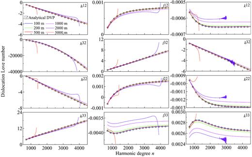
DLNs, with factor (rs/a)n being excluded, due to different types of dislocation source located at depth d ( = a − rs) = 20 km, computed by the analytical DVP method, as compared to the numerical Runge–Kutta technique with different integral steps (i.e. the thickness in each step). The earth model is ISO PREM.

Figure 2.

DLNs, with factor (r_s/a)ⁿ being excluded, due to different types of dislocation source located at depth d ( = a − r_s) = 20 km, computed by the analytical DVP method, as compared to the numerical Runge–Kutta technique with different integral steps (i.e. the thickness in each step). The earth model is ISO PREM.

Open in new tab Download slide

It is observed from Fig. 2 that the numerical DLNs with step size of 5 km are completely wrong when degree n is larger than about 1000. When the step size is 2 km, some DLNs are also wrong. For example, DLN h’s are obviously incorrect when degree n is larger than 3000, and DLN k’s begin to oscillate when n is about 2500. Although stable results can be obtained by the numerical integration when the step size is 1 km, one could still observe some relatively large differences as compared to those using the step size of 100 m. However, when the step size is set to 500 m or smaller (i.e. at 100, 200 and 500 m), the numerically calculated DNLs are closer to the analytical ones. Consequently, for a source depth of 20 km, the step size for the numerical integral method should be 500 m or smaller.

The DNLs computed by our analytical DVP method are also plotted in Fig. 2, which are consistent with the numerical ones using step sizes of 100 and 200 m. This validates the new analytical DVP method introduced in this paper. It should be noted that the original ISO PREM model consisted of less than 100 uniform layers (mantle plus core, with the largest layer thickness being 100 km) which is very small compared to the number of layers used in the numerical integration method (Table 2). As such, the proposed analytical DVP method is much faster than the direct numerical integration approach—at least 3 orders of magnitude faster!

To clearly demonstrate the excellent agreement of the DLNs computed by the analytical and numerical methods, Fig. 3 shows only the DLNs results by the numerical integral method using the step size of 50 m and those from the analytical DVP method, also for a source at depth of 20 km, but with the factor (r_s/a)ⁿ being included (i.e. the same as originally defined in Section 4). To show the results of degree zero for the tensile dislocation in logarithmic axis, n = 0 is shifted to n = 0.8. Again, the excellent agreement between the two methods can be clearly observed.

Figure 3.

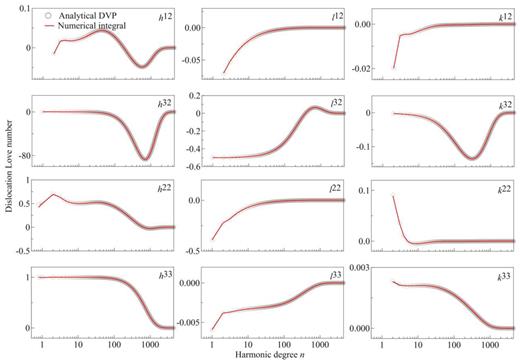
DLNs due to different types of dislocation source located at depth d = a − r_s = 20 km, computed by the analytical DVP method, as compared to the numerical Runge–Kutta technique with the step size of 50 m (i.e. with thickness of 50 m for each layer). The earth model is ISO PREM.

Open in new tab Download slide

6.2 Convergence and surface rupture

Convergence is a key issue when computing Green's functions for a layered Earth. In theory, the summation for the harmonic degree n in the Green's function goes to infinity. However, this is unnecessary because the DNLs tend to zero with increasing degree n, providing that the source depth is greater than zero. Therefore, all the summations involved in the Green's function expression in Section 4 can be always truncated to a relatively large harmonic degree as long as the Green's functions are convergent. Sun & Okubo (1993) provided a very useful criterion: to guarantee an accuracy of about 10⁻⁵ for the Green's function solution, the largest degree n needed is nMax = 10a/d, where d is the source depth and a is the Earth's radius.

To examine the criterion introduced by Sun & Okubo (1993) and to check the capability of our DVP method, we plot in Fig. 4 the source depth versus the converged degrees of the DLNs using the ISO PREM model (using DLN h¹² as example). The lower-degree parts are not presented in order to show clearly the convergence behaviour. It is obvious from Fig. 4 that all the non-zero DLNs at different depths converge to zero when harmonic degree n approaches infinity because of the factor (r_s/a)ⁿ. The inclined solid straight line shows the truncation criterion of Sun & Okubo (1993). Comparing the circles with the inclined line in Fig. 4, it is clear that our DVP method can calculate all the DLNs all the way to a very large degree n which can be much larger than nMax. For instance, for the surface rupture or near surface dislocation, our DVP method can provide DLNs all the way to degree n larger than 1 million! This will guarantee the DLN accuracy by our method to better, say, than 10⁻⁶. Hence the computed DLNs by our method are sufficient to derive the Green's functions with an accuracy of at least 10⁻⁵.

Figure 4.

Relationship between source depth d = a − r_s (in km) and converged harmonic degree n of the DLNs [circles show DLNs; horizontal dash lines are zero lines of the DLNs at different source depths; inclined solid straight line shows the truncation criterion nMax = 10a/d from Sun & Okubo (1993)]. The DLN element h¹² is used to show the convergent trend.

Open in new tab Download slide

Since a fault can reach and cut the surface of the Earth, any computational method needs also to take care of this important special case. This has been a challenge for many existing methods, such as the normal-mode method, because of the convergence issue (Sun & Dong 2013). By making use of the reciprocity theorem, Sun & Dong (2013) derived the relation between the DLNs and the conventional tide, pressure and shear Love numbers to solve this problem. Since the DVP method proposed in this paper is a very stable and flexible one, it can be also applied to this special case directly. For example, Fig. 5 shows all the non-zero spheroidal DLNs versus degree n computed by our DVP method for this specific case (when the source is exactly located on the surface, i.e. d = 0), for degrees n all the way to 1 million. It can be observed from Fig. 5 that: (1) with increasing degree n, all the DLNs converge to their individual limits; (2) for all the DLNs, they converge to their asymptotic limits at different degree n, but they all converge at a degree n which is much smaller than n = 1 million; and (3) these DLN curves are consistent with equations in Section 3 of Sun & Dong (2013), except for the different factors used in defining the DLNs and in defining the vector spherical harmonics. For example, h₃₃= (2n + 1)/(4π) in eq. (66) in Sun & Dong (2013) is exactly identical to our result h³³= 1 as shown in Fig. 5, and similar equivalences can be found for l³² and l^t³². Thus, Fig. 5 shows not only the flexibility of our analytical DVP method to the special surface dislocation case but also its accuracy in calculating the DLNs to a degree n, which can be much larger than the converged one.

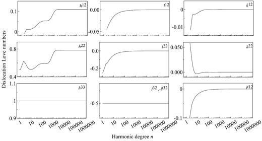
DLNs with source on the surface, that is depth d = 0, where h33, l32 and lt32 are also comparable with those in Sun & Dong (2013).

Figure 5.

DLNs with source on the surface, that is depth d = 0, where h³³, l³² and l^t³² are also comparable with those in Sun & Dong (2013).

Open in new tab Download slide

6.3 Effect of anisotropy

To show the effect of Earth anisotropy on DLNs, we compute two sets of DLNs for both isotropic and transversely isotropic earth models (i.e. using both ISO PREM and TI PREM). The results are depicted in Figs 6 and 7 for the source located at depth 20 and 100 km, respectively.

Figure 6.

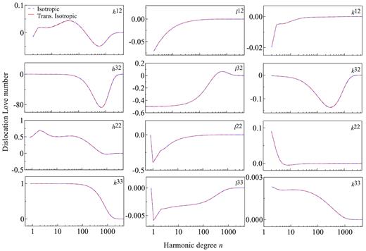
DLNs versus harmonic degree n with source at depth d = 20km: Comparison between isotropic ISO PREM (blue dashed line) and transversely isotropic TI PREM (red solid lines) earth models.

Open in new tab Download slide

Figure 7.

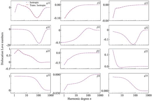
DLNs versus harmonic degree n with source at depth d = 100 km: Comparison between isotropic ISO PREM (blue dashed line) and transversely isotropic TI PREM (red solid lines) earth models.

Open in new tab Download slide

It is observed from Fig. 6 that the effect of anisotropy (as invoked in the model PREM) on all the DLNs can be neglected except for h¹² where slight difference between the two models can be seen when degree n < 100. We note that while the source is at 20 km, the anisotropy is located in the layers ranging from depth 200 to 24.4 km. Therefore, it is natural to ask if the effect of anisotropy on the DLNs would be the same if the source is located in the transversely isotropic layer. Shown in Fig. 7 are the comparison on the DLNs for the two models when the source is located at depth d = 100 km which is within the transversely isotropic layer. Compared to Fig. 6, it is observed from Fig. 7 that all the DLNs by the vertical strike-slip (with superscript pairs 12) are clearly affected by the anisotropy. There are large differences in h¹² for harmonic degree ranging from n = 6 to about 400 (≈ 5 per cent at n = 69) and some differences in l¹² for small degrees, say n < 10. There are also some tiny differences in k¹² and in h²².

To show the difference of the DLNs between ISO and TI PREM models, we exclude the factor (r_s/a)ⁿ and plot the results in Fig. 8 for the same case as shown in Fig. 7. Notice that although for the TI PREM model, the factor will be different from (r_s/a)ⁿ, excluding the same factor out will help to see the difference clearly. It is indeed observed from Fig. 8 that with increasing degree n, the difference in DLNs between ISO and TI PREM models increases. While these differences are suppressed by the factor (r_s/a)ⁿ, the effect of transverse isotropy on the DLNs could be significant when the fault is located in a shallow and anisotropic layer.

Similar to Fig. 7 but with factor (rs/a)n being excluded from both ISO and TI DLNs.

Figure 8.

Similar to Fig. 7 but with factor (r_s/a)ⁿ being excluded from both ISO and TI DLNs.

Open in new tab Download slide

Again while in general the effect of anisotropy is relatively small based on the global TI PREM model, the capability of the present formulation and the corresponding MATLAB code with anisotropy would have potential applications in the following three areas: (1) due to the imbalance between tectonic stress and strain rate and other tectonic features, the effective properties of the rock materials could be strongly anisotropic (Cambiotti et al.2014), which could substantially alter the fault-induced response away from those of the isotropic model; (2) in the regional scale, many rocks in the lithosphere are also anisotropic (Pan et al.2014), and the influence of rock anisotropy can be strong; and (3) viscous anisotropy of the mantle materials could be very strong when studying the corresponding viscoelastic response (Hansen et al.2012).

7 CONCLUSIONS

We have developed an analytical method to compute all the DLNs using a special matrix propagating approach called DVP, for a spherically symmetric, non-rotating, perfectly elastic, transversely isotropic and self-gravitating Earth. Numerical comparisons show that the results computed by DVP method are in good agreement with those based on the other methods. However, the analytical DVP method is more stable and much faster than the alternatives.

As demonstrated in this paper, our software can calculate the DNLs to an arbitrarily high degree n so as to guarantee that the corresponding elastic dislocation Green's function can be computed with an accuracy of at least 10⁻⁵. Furthermore, our analytical DNLs are applicable to a surface rupture, that is when the point dislocation is located exactly on the Earth's surface.

The effect of the upper-mantle anisotropy of the Earth on the fault DNLs is very minor, except if the fault is vertical strike-slip located within the anisotropic layer.

SUPPORTING INFORMATION

GJI Paper I on DLNs Code and Manual Revised 0226 2019.docx

Figure S1. Comparison of the DLNs between the PREM and STW105 earth models for a point dislocation located at depth d = 20 km.

Table S1. Comparison of DLN h¹² (different degrees n) for the point dislocation located at depth 20 km in the homogeneous mantle which is, respectively, subdivided into 129, 1025 and 16385 sublayers.

Table S2. Comparison of DLN l¹² (different degrees n) for the point dislocation located at depth 20 km in the homogeneous mantle which is, respectively, subdivided into 129, 1025 and 16385 sublayers.

Table S3. Comparison of DLN k¹² (different degrees n) for the point dislocation located at depth 20 km in the homogeneous mantle which is, respectively, subdivided into 129, 1025 and 16385 sublayers.

Please note: Oxford University Press is not responsible for the content or functionality of any supporting materials supplied by the authors. Any queries (other than missing material) should be directed to the corresponding author for the paper.

ACKNOWLEDGEMENTS

This study was financially supported by the National Natural Science Foundation of China projects (Grant Nos 41621091 and 41874026) (J. Zhou). The authors would like to thank the handling editor and the two reviewers for their constructive comments which have been very helpful in modifying the original version.

REFERENCES

Ai

Z.Y.

,

Cheng

Y.C.

,

2014

.

Extended precise integration method for consolidation of transversely isotropic poroelastic layered media

,

Comput. Math. Appl.

,

68

,

1806

–

1818

..

10.1016/j.camwa.2014.10.010

Aki

K.

,

Richards

P.G.

,

1980

.

Quantitative Seismology Theory and Methods

,

Vol. I

,

W. H. Freeman and Company

.

Google Scholar

Google Preview

OpenURL Placeholder Text

WorldCat

Ben-Menahem

A.

,

Singh

S.J.

,

1981

.

Seismic Waves and Sources

,

Springer-Verlag

Google Scholar

Google Preview

OpenURL Placeholder Text

WorldCat

Berry

D.S.

,

Sales

T.W.

,

1962

.

An elastic treatment of ground movement due to mining. III. Three dimensional problem, transversely isotropic ground

,

J. Mech. Phys. Solids

,

10

,

73

–

83

..

10.1016/0022-5096(62)90030-3

Cambiotti

G.

,

Sabadini

R.

,

2015

.

On the response of the Earth to a fault system: its evaluation beyond the epicentral reference frame

,

Geophys. J. Int.

,

203

,

943

–

959

..

Cambiotti

G.

,

Barletta

V.R.

,

Bordoni

A.

,

Sabadini

R.

,

2009

.

A comparative analysis of the solutions for a Maxwell Earth: the role of the advection and buoyancy force

,

Geophys. J. Int.

,

176

,

995

–

1006

..

10.1111/j.1365-246X.2008.04034.x

Cambiotti

G.

,

Rigamonti

S.

,

Splendore

R.

,

Marotta

A.M.

,

Sabadini

R.

,

2014

.

Power-law Maxwell rheologies and the interaction between tectonic and seismic deformations

,

Geophys. J. Int.

,

198

,

1293

–

1306

..

Cambiotti

G.

,

Wang

X.

,

Sabadini

R.

,

Yuen

D.A.

,

2016

.

Residual polar motion caused by coseismic and interseismic deformations from 1900 to present

,

Geophys. J. Int.

,

205

,

1165

–

1179

..

Chao

B.F.

,

Gross

R.S.

,

1987

.

Changes in the Earth's rotation and low-degree gravitational field induced by earthquakes

,

Geophys. J. R. astr. Soc.

,

91

,

569

–

596

..

10.1111/j.1365-246X.1987.tb01659.x

Chen

J.Y.

,

Pan

E.

,

Bevis

M.

,

2018

.

Accurate computation of the elastic load Love numbers to high spectral degree for a finely layered, transversely isotropic and self-gravitating Earth

,

Geophys. J. Int.

,

212

,

827

–

838

.

Davis

P.M.

,

1983

.

Surface deformation associated with a dipping hydrofracture

,

J. geophys. Res.

,

88

,

5826

–

5834

..

10.1029/JB088iB07p05826

Dziewonski

A.M.

,

Anderson

D.L.

,

1981

.

Preliminary reference Earth model

,

Phys. Earth planet. Inter.

,

25

,

297

–

356

..

10.1016/0031-9201(81)90046-7

Farrell

W.E.

,

1972

.

Deformation of the Earth by surface loads

,

Rev. Geophs. Phys.

,

10

(

3

),

761

–

797

..

10.1029/RG010i003p00761

Fukahata

Y.

,

Matsu'ura

M.

,

2005

.

General expressions for internal deformation fields due to a dislocation source in a multilayered elastic half-space

,

Geophys. J. Int.

,

161

,

507

–

521

..

10.1111/j.1365-246X.2005.02594.x

Gilbert

F.

,

Backus

G.

1968

.

Elastic-gravitational vibrations of a radially stratified sphere

, in

Dynamics of Stratified Solids

, pp.

82

–

95

.ed.

Herrmann

G.

,

American Society of Mechanical Engineers

.

Google Scholar

Google Preview

OpenURL Placeholder Text

WorldCat

Gomez

D.D.

,

Bevis

M.

,

Pan

E.

,

Smalley

R.

,

2017

.

The influence of gravity on the displacement field produced by fault slip

,

Geophys. Res. Lett.

,

44

,

9321

–

9329

..

Gross

R.S.

,

Chao

B.F.

,

2006

.

The rotational and gravitational signature of the December 26, 2004 Sumatran earthquake

,

Surv. Geophys.

,

27

,

615−632

.

10.1007/s10712-006-9008-1

Han

S.

,

Shum

C.K.

,

Bevis

M.

,

Ji

C.

,

Kuo

C.

,

2006

.

Crustal dilatation observed by GRACE after the 2004 Sumatra-Andaman Earthquake

,

Science

,

313

,

658

–

662

..

10.1126/science.1128661

Hansen

L.N.

,

Zimmerman

M.E.

,

Kohlstedt

D.L.

,

2012

.

Laboratory measurements of the viscous anisotropy of olivine aggregates

,

Nature

,

492

(

7429

),

415

–

418

..

Heiskanen

W.A.

,

Moritz

H.

,

1967

.

Physical Geodesy

,

W. H. Freeman and Company

Google Scholar

Google Preview

OpenURL Placeholder Text

WorldCat

Heki

K.

,

Matsuo

K.

,

2010

.

Coseismic gravity changes of the 2010 earthquake in central Chile from satellite gravimetry

,

Geophy. Res. Lett.

,

37

,

L24306

,

doi: 10.1029/2010GL045335

.

Imanishi

Y.

,

Sato

T.

,

Higashi

T.

,

Sun

W.

,

Okubo

S.

,

2004

.

A network of superconducting gravimeters detects submicrogal coseismic gravity changes

,

Science

,

306

,

476

–

478

..

10.1126/science.1101875

Kennett

B.L.N.

,

1983

.

Seismic Wave Propagation in Stratified Media

,

Cambridge University Press

.

Google Scholar

Google Preview

OpenURL Placeholder Text

WorldCat

Liu

H.

,

Pan

E.

,

Cai

Y.

,

2018

.

General surface loading over layered transversely isotropic pavements with imperfect interfaces

,

Adv. Eng. Software

,

115

,

268

–

282

..

10.1016/j.advengsoft.2017.09.009

Love

A.E.H.

1911

.

Some Problems of Geodynamics

,

Cambridge University Press

.

Google Scholar

Google Preview

OpenURL Placeholder Text

WorldCat

Lynner

C.

,

Beck

S.L.

,

Zandt

G.

,

Porritt

R.W.

,

Lin

F.C.

,

Eilon

Z.C.

,

2018

.

Midcrustal deformation in the central Andes constrained by radial anisotropy

,

J. geophys. Res.: Solid Earth

,

123

,

doi.org/10.1029/2017JB014936

.

Google Scholar

OpenURL Placeholder Text

WorldCat

Maruyama

T.

,

1964

.

Static elastic dislocation in an infinite and semi-infinite demium

,

Bull. Earthq. Res. Inst. Univ. Tokyo

,

42

,

289

–

368

.

Google Scholar

OpenURL Placeholder Text

WorldCat

Meade

B.J.

,

2007

.

Algorithms for the calculation of exact displacements, strains, and stresses for triangular dislocation elements in a uniform elastic half space

,

Comput. Geosci.

,

33

(

8

),

1064

–

1075

..

10.1016/j.cageo.2006.12.003

Melini

D.

,

Spada

G.

,

Piersanti

A.

,

2010

.

A sea level equation for seismic perturbations

,

Geophys. J. Int.

,

180

,

88

–

100

..

10.1111/j.1365-246X.2009.04412.x

Nikkhoo

M.

,

Walter

T.R.

,

2015

.

Triangular dislocation: an analytical, artifact-free solution

,

Geophys. J. Int.

,

201

,

1119

–

1141

..

Okada

Y.

,

1992

.

Internal deformation due to shear and tensile faults in a half-space

,

Bull. seism. Soc. Am.

,

82

,

1018

–

1040

.

Google Scholar

OpenURL Placeholder Text

WorldCat

Okada

Y.

,

1985

.

Surface deformation caused by shear and tensile faults in a half-space

,

Bull. seism. Soc. Am.

,

75

,

1135

–

1154

.

Google Scholar

OpenURL Placeholder Text

WorldCat

Okubo

S.

,

Endo

T.

,

1986

.

Static spheroidal deformation of degree 1 – consistency relation, stress solution and partials

,

Geophys. J. R. astr. Soc.

,

86

,

91

–

102

..

10.1111/j.1365-246X.1986.tb01074.x

Okubo

S.

,

1991

.

Potential and gravity changes raised by point dislocations

,

Geophys. J. Int.

,

105

,

573

–

586

..

10.1111/j.1365-246X.1991.tb00797.x

Okubo

S.

,

1992

.

Potential and gravity changes caused by shear and tensile faults

,

J. geophys. Res.

,

97

,

7137

–

7144

..

Okubo

S.

,

1993

.

Reciprocity theorem to compute the static deformation due to a point dislocation buried in a spherically symmetric Earth

,

Geophys. J. Int.

,

115

,

921

–

928

..

10.1111/j.1365-246X.1993.tb01501.x

Pan

E.

,

1989

.

Static response of a transversely isotropic and layered halfspace to general dislocation sources

,

Phys. Earth planet. Inter.

,

58

,

103

–

117

..

10.1016/0031-9201(89)90046-0

Pan

E.

,

1991

.

Dislocation in an infinite poroelastic medium

,

Acta Mech.

,

87

,

105

–

115

..

Pan

E.

,

Chen

W.Q.

,

2015

.

Static Green's Functions in Anisotropic Media

,

Cambridge University Press

.

Google Scholar

Google Preview

OpenURL Placeholder Text

WorldCat

Pan

E.

,

Yuan

J.H.

,

Chen

W.Q.

,

Griffith

W.A.

,

2014

.

Elastic deformation due to polygonal dislocations in a transversely isotropic half-space

,

Bull. seism. Soc. Am.

,

104

,

2698

–

2716

..

Pan

E.

,

Molavi Tabrizi

A.

,

Sangghaleh

A.

,

Griffith

W.A.

,

2015a

.

Displacement and stress fields due to finite shear and tensile faults in an anisotropic elastic half-space

,

Geophys. J. Int.

,

203

,

1193

–

1206

..

Pan

E.

,

Chen

J.Y.

,

Bevis

M.

,

Bordoni

A.

,

Barletta

V.R.

,

Molavi Tabrizi

A.

,

2015b

.

An analytical solution for the elastic response to surface loads imposed on a layered, transversely isotropic, and self-gravitating Earth

,

Geophys. J. Int.

,

203

,

2150

–

2181

..

Pan

E.

,

Liu

H.

,

Zhang

Z.Q.

,

2018

.

Vertical and torsional vibrations of a rigid circular disc on a transversely isotropic and layered half-space with imperfect interfaces

,

Soil Dyn. Earthq. Eng.

,

113

,

442

–

453

..

10.1016/j.soildyn.2018.06.014

Pollitz

F.F.

,

1992

.

Postseismic relaxation theory on the spherical earth

,

Bull. Seismol. Soc. Am.

,

82

,

422

–

453

.

Google Scholar

OpenURL Placeholder Text

WorldCat

Press

F.

,

1965

.

Displacements, strains and tilts at teleseismic distances

,

J. Geophys. Res.

,

70

,

2395

–

2412

..

10.1029/JZ070i010p02395

Sabadini

R.

,

Vermeersen

L.L.A.

,

1997

.

Influence of lithospheric and mantle stratification on global post-seismic deformation

,

Geophys. Res. Lett.

,

24

,

2075

–

2078

..

Sabadini

R.

,

Vermeersen

B.

,

Cambiotti

G.

,

2016

.

Global Dynamics of the Earth: Applications of Viscoelastic Relaxation Theory to Solid-Earth and Planetary Geophysics

,

Vol. 20

,

Springer

,

ISBN:9789401775526, doi:10.1007/978-94-017-7552-6

.

Google Scholar

Google Preview

OpenURL Placeholder Text

WorldCat

Singh

S.J.

,

1970

.

Static deformation of a multilayered half-space by internal sources

,

J. geophys. Res.

,

75

,

3257

–

3263

..

10.1029/JB075i017p03257

Steketee

J.A.

,

1958

.

On Volterra's dislocations in a semi-infinite elastic medium

,

Can. J. Phys.

,

36

,

192

–

205

..

Sun

W.

,

1992

.

Potential and gravity changes caused by dislocations in spherically symmetric earth models

,

Bull. Earthq. Res. Inst. Univ. Tokyo

,

67

,

89

–

238

.

Google Scholar

OpenURL Placeholder Text

WorldCat

Sun

W.

,

2003

.

Asymptotic theory for calculating deformations caused by dislocations buried in a spherical earth: Geoid change

,

J. Geod.

,

77

(

7–8

),

381

–

387

..

10.1007/s00190-003-0335-4

Sun

W.

,

2004a

.

Asymptotic solution of static displacements caused by dislocations in a spherically symmetric Earth

,

J. geophys. Res.

,

109

,

B05402

,

doi.org/10.1029/2003JB002793

.

Google Scholar

OpenURL Placeholder Text

WorldCat

Sun

W.

,

2004b

.

Short note: asymptotic theory for calculating deformations caused by dislocations buried in a spherical earth—Gravity change

,

J. Geod.

,

78

(

1

),

76

–

81

.

Google Scholar

OpenURL Placeholder Text

WorldCat

Sun

W.

,

Okubo

S.

,

1993

.

Surface potential and gravity changes due to internal dislocations in a spherical Earth, 1. Theory for a point dislocation

,

Geophys. J. Int.

,

114

,

569

–

592

..

10.1111/j.1365-246X.1993.tb06988.x

Sun

W.

,

Okubo

S.

,

2002

.

Effects of the Earth's spherical curvature and radial heterogeneity in dislocation studies for a point dislocation

,

Geophys. Res. Lett.

,

29

,

1605

.

Sun

W.

,

Okubo

S.

,

2004

.

Coseismic deformations detectable by satellite gravity missions: A case study of Alaska (1964, 2002) and Hokkaido (2003) earthquakes in the spectral domain

,

J. geophys. Res.

,

109

,

B04405

,

doi:10.1029/2003JB002554

.

Google Scholar

OpenURL Placeholder Text

WorldCat

Sun

W.

,

Dong

J.

,

2013

.

Relation of dislocation Love numbers and conventional Love numbers and corresponding Green's functions for a surface rupture in a spherical earth model

,

Geophys. J. Int.

,

193

,

717

–

733

..

Sun

W.

,

Okubo

S.

,

Vaníček

,

1996

.

Global displacements caused by point dislocations in a realistic Earth model

,

J. geophys. Res.

,

101

(

B4

),

8561

–

8577

..

Takeuchi

H.

,

Saito

M.

,

1972

.

Seismic surface waves

, in

Methods in Computational Physics

,

Vol. 11

, pp.

217

–

295

., ed.

Bolt

B.A.

,

Academic Press

.

Google Scholar

Google Preview

OpenURL Placeholder Text

WorldCat

Tanaka

Y.

,

Okuno

J.

,

Okubo

S.

2006

.

A new method for the computation of global viscoelastic post-seismic deformation in a realistic earth model (I)-vertical displacement and gravity variation

,

Geophys. J. Int.

,

164

,

273

–

289

..

10.1111/j.1365-246X.2005.02821.x

Tang

H.

,

Sun

W.

,

2017

.

Asymptotic expressions for changes in the surface co-seismic strain on a homogeneous sphere

,

Geophy. J. Int.

,

209

(

1

),

ggx006

–

ggx225

..

Tang

H.

,

Sun

W.

,

2018

.

Asymptotic co- and post-seismic displacements in a homogeneous Maxwell sphere

,

Geophys. J. Int.

,

214

,

731

–

750

..

Tapley

B.D.

,

Bettadpur

S.

,

Ries

J.C.

,

Thompson

P.F.

,

Watkins

M.

,

2004

.

GRACE measurements of mass variability in the Earth system

,

Science

,

305

(

5683

),

503

–

505

..

10.1126/science.1099192

Wang

H.

,

1999

.

Surface vertical displacements, potential perturbations and gravity changes of a viscoelastic earth model induced by internal point dislocations

,

Geophys. J. Int.

,

137

,

429

–

440

..

10.1046/j.1365-246X.1999.00797.x

Wang

R.

,

Lorenzo-Martín

F.

,

Roth

F.

,

2006

.

PSGRN/PSCMP—a new code for calculating co- and post-seismic deformation, geoid and gravity changes based on the viscoelastic-gravitational dislocation theory

,

Comput. Geosci.

,

32

,

527

–

541

..

10.1016/j.cageo.2005.08.006

Wu

P.

,

Peltier

W.R.

,

1982

.

Viscos gravitational relaxation

,

Geophys. J. R. astr. Soc.

,

70

,

435

–

485

..

10.1111/j.1365-246X.1982.tb04976.x

Xu

C.

,

Sun

W.

,

2014

.

Earthquake-origin expansion of the Earth inferred from a spherical-Earth elastic dislocation theory

,

Geophys. J. Int.

,

199

,

1655

–

1661

..

Xu

C.

,

Chao

B.F.

,

2017

.

Coseismic changes of gravitational potential energy induced by global earthquakes based on spherical-Earth elastic dislocation theory

,

J. geophys. Res.

,

122

(

5

),

4053

–

5063

..

Yamazaki

K.

,

1978

.

Theory of crustal deformation due to dilatancy and quantitative evaluation of earthquake precursors

,

Sci. Rep. Tohoku Univ., Ser. 5, Geophys.

,

25

,

115

–

167

.

Google Scholar

OpenURL Placeholder Text

WorldCat

Zhong

W.X.

,

Lin

J.H.

,

Gao

Q.

,

2004

.

The precise computation for wave propagation in stratified materials

,

Int. J. Numerical Methods Eng.

,

60

,

11

–

25

..

Zhou

J.

,

Sun

W.

,

Sun

H.

,

Xu

J.

,

2013

.

Reformulation of co-seismic polar motion excitation and low degree gravity changes: applied to the 2011 Tohoku-Oki earthquake (Mw9.0)

,

J. Geodyn.

,

63

,

20

–

26

..

10.1016/j.jog.2012.09.004

Zhou

J.

,

Sun

W.

,

Sun

H.

,

Xu

J.

,

Cui

X.

2014

.

Co-seismic change of length of day based on the point dislocation theory for a SNREI Earth

,

J. Geodyn.

,

79

,

18

–

22

..

10.1016/j.jog.2014.04.012

Zhou

J.

,

Sun

W.

,

Dong

J.

,

2015

.

A Correction to the article “Geocenter movement caused by huge earthquakes” by Sun and Dong

,

J. Geodyn.

,

87

,

67

–

73

..

10.1016/j.jog.2015.02.003

Zhou

J.

,

Sun

W.

,

Jin

S.

,

Sun

H.

,

Xu

J.

,

2016

.

Rotation change in the orientation of the center-of-figure frame caused by large earthquakes

,

Geophys. J. Int.

,

206

,

999

–

1008

..

Zhou

J.

,

Sun

H.

,

Xu

J.

,

Cui

X.

,

Chen

X.

,

2017

.

Co-seismic gravitational potential energy change and its tectonic implications: a case study in Tibetan plateau area

,

Chin. J. Geophys.

,

60

(

3

),

313

–

320

..

APPENDIX A: VECTOR SPHERICAL HARMONICS

To solve the problem in spherical and layered Earth, we employ the spherical system of vector functions (or vector spherical harmonics) in terms of the spherical coordinates (r,θ,ϕ). These vector functions are defined as

\begin{eqnarray*} \left. {\begin{array}{@{}*{1}{c}@{}} {\begin{array}{@{}*{1}{c}@{}} {{\boldsymbol{L}}\ \left( {\theta ,\phi ;n,m} \right) = {{\boldsymbol{e}}_r}\ S\ \left( {\theta ,\phi ;n,m} \right) = {{\boldsymbol{e}}_r}\ S}\\ {{\boldsymbol{M}}\left( {\theta ,\phi ;n,m} \right) = r\nabla S = {{\boldsymbol{e}}_\theta }\ \displaystyle\frac{{\partial S}}{{\partial \theta }} + {{\boldsymbol{e}}_\phi }\displaystyle\frac{{\partial S}}{{{\rm{sin}}\theta \partial \phi }}} \end{array}}\\ {N\ \left( {\theta ,\phi ;n,m} \right) = r\nabla \times \left( {{{\boldsymbol{e}}_r}S} \right) = {{\boldsymbol{e}}_\theta }\ \displaystyle\frac{{\partial S}}{{{\rm{sin}}\theta \partial \phi }} - {{\boldsymbol{e}}_\phi }\displaystyle\frac{{\partial S}}{{\partial \theta }}} \end{array}} \right\}, \end{eqnarray*}

(A1)

where e_r, e_θ and e_ϕ are the unit vectors, respectively, along r-, θ- and ϕ-directions, and S is a scalar function defined by

\begin{eqnarray*} S\left( {\theta ,\phi ;n,m} \right) = \sqrt {\frac{{\left( {2n + 1} \right)\left( {n - m} \right)!}}{{4\pi \left( {n + m} \right)!}}} \ P_n^m\left( {{\rm{cos}}\theta } \right){e^{im\phi}} \equiv \bar{P}_n^m\left( {{\rm{cos}}\theta } \right){e^{im\phi}},\ \quad \left| m \right| \le n;n = 0,1,2, \ldots \end{eqnarray*}

(A2)

The associated Legendre function |$P_n^m$| in eq. (A2) is defined as

\begin{eqnarray*} P_n^m\ \left( x \right) = {\left( { - 1} \right)^m}\ {\left( {1 - {x^2}} \right)^{m/2}}\frac{{{{\rm{d}}^m}}}{{{\rm{d}}{x^m}}}{P_n}\left( x \right),\ \ \ m \ge 0, \end{eqnarray*}

(A3)

where P_n is the Legendre function of degree n. eq. (A2) holds for any positive m; when this index is negative, the associated function is defined in terms of its positive one as

\begin{eqnarray*} \bar{P}_n^{ - m}\ \left( x \right) = {\left( { - 1} \right)^m}\ \frac{{\left( {n - m} \right)!}}{{\left( {n + m} \right)!}}\bar{P}_n^m\left( x \right),\ \ m \ge 0 . \end{eqnarray*}

(A4)

In so doing, one can define

\begin{eqnarray*} S\ \left( {\theta ,\phi ;n, - m} \right) = {\left( { - 1} \right)^m}\ {S^*}\left( {\theta ,\phi ;n,m} \right), \end{eqnarray*}

(A5)

where an asterisk denotes complex conjugate, giving as

\begin{eqnarray*} {S^*}\left( {\theta ,\phi ;n,m} \right) = \bar{P}_n^m\ \left( {{\rm{cos}}\theta } \right){e^{ - im\phi}},\quad \left| m \right| \le n;n = 0,1,2, \ldots \end{eqnarray*}

(A6)

Since eq. (A1) forms an orthonormal vector system, any vector can be expanded in terms of it. As an example, the body-force vector f can be expressed as

\begin{eqnarray*} {\boldsymbol{f\ }}\left( {r,\theta ,} \right) = \mathop \sum \nolimits_{{\rm{n}} = 0}^\infty \mathop \sum \nolimits_{{\rm{m}} = - {\rm{n}}}^{\rm{n}} \left[ {{F_L}\left( r \right){\boldsymbol{L}}\left( {\theta ,\phi ;n,m} \right) + {F_M}\left( r \right){\boldsymbol{M}}\left( {\theta ,\phi ;n,m} \right) + {F_N}\left( r \right){\boldsymbol{N}}\left( {\theta ,\phi ;n,m} \right)} \right] \end{eqnarray*}

(A7)

in which the expansion coefficients are

\begin{eqnarray*} \left. {\begin{array}{@{}*{1}{c}@{}} {{F_L}\ \left( {r,n,m} \right) = \mathop \int \nolimits_0^{2{\rm{\pi }}} \mathop \int \nolimits_0^{\rm{\pi }} {\boldsymbol{f}}\left( {r,\theta ,} \right) \cdot {\boldsymbol{\ }}{{\boldsymbol{L}}^{\boldsymbol{*}}}\left( {\theta ,\phi ;n,m} \right){\rm{sin}}\theta {\rm{d}}\theta {\rm{d\phi}}}\\ {{F_M}\ \left( {r,n,m} \right) = \displaystyle\frac{1}{{n\left( {n + 1} \right)}}\ \mathop \smallint \nolimits_0^{2{\rm{\pi }}} \mathop \smallint \nolimits_0^{\rm{\pi }} {\boldsymbol{f}}\left( {r,\theta ,} \right) \cdot {{\boldsymbol{M}}^{\boldsymbol{*}}}\left( {\theta ,\phi ;n,m} \right){\rm{sin}}\theta {\rm{d}}\theta {\rm{d\phi}}}\\ {{F_N}\ \left( {r,n,m} \right) = \displaystyle\frac{1}{{n\left( {n + 1} \right)}}\ \mathop \smallint \nolimits_0^{2{\rm{\pi }}} \mathop \smallint \nolimits_0^{\rm{\pi }} {\boldsymbol{f}}\left( {r,\theta ,} \right) \cdot {{\boldsymbol{N}}^{\boldsymbol{*}}}\left( {\theta ,\phi ;n,m} \right){\rm{sin}}\theta {\rm{d}}\theta {\rm{d\phi}}} \end{array}} \right\}, \end{eqnarray*}

(A8)

where the dot means inner product.

APPENDIX B: SPECIAL TREATMENTS FOR DEGREES n = 0 AND n = 1

B1 For degree n = 0

For degree n = 0, there's only spheroidal deformation while the toroidal one vanishes. In this case, the six differential equations governing the Earth deformation degenerate to three equations as

\begin{eqnarray*} {{U{^{\prime}}}_L} &=& - \frac{{2{c_{13}}}}{{{c_{33}}}}\frac{{{U_L}}}{r} + \frac{{{T_L}}}{{{c_{33}}}} \nonumber \\ {{T{^{\prime}}}_L} &=& - \frac{{4\rho g{U_L}}}{r} + \frac{{2\left[ {{c_{33}}\left( {{c_{11}} + {c_{12}}} \right) - 2c_{13}^2} \right]{U_L}}}{{{c_{33}}{r^2}}} + \frac{2}{r}\left( {\frac{{{c_{13}}}}{{{c_{33}}}} - 1} \right){T_L} \nonumber \\ {\rm{\Phi {^{\prime}}}} &=& - 4{\rm{\pi G\rho }}{U_L} . \end{eqnarray*}

(B1)

It is observed that the third equation in eq. (B1) is decoupled from the first two and hence it can be solved separately after the first two are solved.

Furthermore, in the homogeneous solid inner core, we assume that the inner core is isotropic. Then the first two equations in eq. (B1) become

\begin{eqnarray*} \quad {{U{^{\prime}}}_L} &=& - \frac{{2\lambda }}{{\lambda + 2\mu }}\frac{{{U_L}}}{r} + \frac{{{T_L}}}{{\lambda + 2\mu }}\nonumber \\ {{T{^{\prime}}}_L} &=& - \frac{{4\rho g{U_L}}}{r} + \frac{{4\mu \left( {3\lambda + 2\mu } \right)}}{{\lambda + 2\mu }}\frac{{{U_L}}}{{{r^2}}} - \frac{{4\mu }}{{\lambda + 2\mu }}\frac{{{T_L}}}{r} . \end{eqnarray*}

(B2)

Love (1911) derived the analytical solutions of eq. (B2) by assuming that the Earth is a homogeneous and isotropic elastic sphere. These solutions can be directly used here for the dislocation-induced deformation of degree n = 0.

On the other hand, in the liquid outer core where μ = 0, eq. (B2) changes to

\begin{eqnarray*} {{U{^{\prime}}}_L} &=& - \frac{{2{U_L}}}{r} + \frac{{{T_L}}}{\lambda } \nonumber \\ {{T{^{\prime}}}_L} &=& - \frac{{4\rho g{U_L}}}{r} . \end{eqnarray*}

(B3)

The general solution of eq. (B3) is

\begin{eqnarray*} \left[ {\begin{array}{@{}*{1}{c}@{}} {{U_L}}\\ {r{T_L}} \end{array}} \right] = \left[ {\begin{array}{@{}*{2}{c}@{}} {{j_1}\left( {br} \right)}& \quad {{y_1}\left( {br} \right)}\\ {\lambda \left[ {br{{j{^{\prime}}}_1}\left( {br} \right) + 2{j_1}\left( {br} \right)} \right]}& \quad {\lambda \left[ {br{{y{^{\prime}}}_1}\left( {br} \right) + 2{y_1}\left( {br} \right)} \right]} \end{array}} \right]\ \left[ {\begin{array}{@{}*{1}{c}@{}} {{c_1}}\\ {{c_2}} \end{array}} \right], \end{eqnarray*}

(B4)

where j₁ and y₁ are the first-order spherical Bessel functions of first and second kinds, respectively, and a prime means derivative with respect to x = br, with

\begin{eqnarray*} b = \sqrt {4\rho k/\lambda } \end{eqnarray*}

(B5)

in which k = g/r is a constant since we assume that gravity g is linear to r in the core. The two coefficients c₁ and c₂ can be determined by the boundary conditions at the inner and outer sides of this liquid core. For the layered liquid core case, these constants are connected by the expansion coefficients on both sides of the layer and then the new DVP method proposed in this paper can be applied to find the solution in the layered liquid core.

We now look at eq. (B1) again in the mantle: We assume that g is constant while |$\rho \ = \bar{\rho }\ \bar{r}/r$| in each layer, in which |$\bar{\rho }$| is the volumetrically averaged density of the layer and |$\bar{r}$| is a constant constrained by mass conservation in the layer. For this case, eq. (B1) changes to

\begin{eqnarray*} {{U{^{\prime}}}_L} &=& - \frac{{2{c_{13}}}}{{{c_{33}}}}\frac{{{U_L}}}{r} + \frac{{{T_L}}}{{{c_{33}}}} \nonumber \\ {{T{^{\prime}}}_L} &=& - \frac{{4\bar{\rho }\bar{r}g{U_L}}}{{{r^2}}} + \frac{{2\left[ {{c_{33}}\left( {{c_{11}} + {c_{12}}} \right) - 2c_{13}^2} \right]{U_L}}}{{{c_{33}}{r^2}}} + \frac{2}{r}\left( {\frac{{{c_{13}}}}{{{c_{33}}}} - 1} \right){T_L} . \end{eqnarray*}

(B6)

Applying the variable transform as in Pan et al. (2015b), eq. (B6) can be changed to a set of differential equations with constant coefficients. Accordingly, the procedures are similar to those in Section 2 for n > 1 (but with a different and small matrix size).

B2 For degree n = 1

For n = 1, it contains a rigid-body motion. First, it can be shown that the following consistency relation holds (Farrell 1972; Okubo & Endo 1986).

\begin{eqnarray*} {T_L} + 2{T_M} - \frac{{4{\rm{\pi G}}}}{g}Q = 0. \end{eqnarray*}

(B7)

This indicates actually that the total force/traction acting on the Earth is zero, that is in equilibrium. As such, there are only two, instead of three, boundary conditions on the Earth's surface that are independent. Next, we choose two arbitrary initial solutions, i.e. two columns in the 6 × 3 matrix on the right-hand side of eq. (17a), and propagate them from the core–mantle boundary directly to the Earth's surface as done in Takeuchi & Saito (1972). The solutions thus obtained are called general solutions. Similarly, the source functions are also propagated from the source level to the Earth's surface. These solutions obtained are called particular solutions. Yet another solution is the rigid-body motion, which is [a, a, ag, 0, 0, 0]^T. Finally, we combine the general, particular and rigid-body solutions together to satisfy the boundary conditions T(a) = 0 and Φ(a) = 0 on the surface. The latter condition means that the origin of the coordinate system is fixed on the centre of mass of the earth model. With the determined combination coefficients, the expansion coefficients U(a) on the surface can thus be derived.

It is interesting that if the second and third columns in eq. (17a) are chosen, one can find that the inner solid core contributes nothing to degree n = 1 solution. Generally, the solution has nothing to do with the inner solid core except for the parameters on the core side at the core–mantle boundary.

The toroidal solution for n = 1 is also special because it is analytical and can be derived directly from the given earth model. Regarding the dislocation as an internal (equivalent) force source, we require that there's no net external force acting on the Earth system. As such, the angular momentum of the Earth conserves, that is (Zhou et al.2016)

\begin{eqnarray*} \mathop \int \nolimits_0^a \mathop \int \nolimits_0^{2\pi } \mathop \int \nolimits_0^\pi \left( {\rho {\boldsymbol{r}} \times {\boldsymbol{u}}} \right){r^2}{\rm{sin}}\theta {\rm{d}}\theta{\rm{d}\phi} {\rm{d}}r = \rm{0} , \end{eqnarray*}

(B8)

where u is the displacement field caused by the dislocation and the volumetric integral is on the entire Earth. It was shown that, due to the spherical symmetry and orthogonality of the vector spherical harmonics, only a vertical dip-slip dislocation can induce non-zero displacements of n = 1 (Zhou et al.2016).

To determine the induced displacements, we look at the corresponding differential equations which govern the deformation

\begin{eqnarray*} {{U{^{\prime}}}_N} &=& \frac{{{U_N}}}{r}\ + \frac{{{T_N}}}{\mu } \nonumber \\ {{T{^{\prime}}}_N} &=& - \frac{{3{T_N}}}{r} . \end{eqnarray*}

(B9)

It is obvious that T_N = 0 in the mantle due to the fact that T_N = 0 on the core–mantle boundary and on the Earth's surface. This means that

\begin{eqnarray*} {U_N} = {b_1}\ r,\ {r_c} \le r \le r_s^ - ;\ \ {U_N} = {b_2}\ r,\ r_s^ + \le r \le a \end{eqnarray*}

(B10)

in which b₁ and b₂ are unknowns, which can be determined by the following conditions.

First, according to the source function, we have

\begin{eqnarray*} {b_2}\ {r_s} - {b_1}\ {r_s} = {\rm{\Delta }}{U_N} . \end{eqnarray*}

(B11)

Secondly, making use of eq. (B8), we have

\begin{eqnarray*} {b_2}\left[ {f\left( a \right) - f\left( {{r_s}} \right)} \right] + {b_1}\ \left[ {f\left( {{r_s}} \right) - f\left( {{a_c}} \right)} \right] = 0 , \end{eqnarray*}

(B12)

where

\begin{eqnarray*} f\left( r \right) = \int \nolimits_0^r \rho {r^4}{\rm{d}}r . \end{eqnarray*}

(B13)

Finally therefore, the unknowns b_i are determined from eqs (B11) and (B12), and the toroidal solution of n = 1 is obtained.

APPENDIX C: SOURCE FUNCTIONS

According to the method presented in Section 3, one can derive the source functions of different kinds of dislocation. The derivation is straightforward but tedious. We list below the final expressions of the source functions for a point dislocation in a transversely isotropic medium (with elastic constants c_ij):

\begin{eqnarray*} {\rm{\Delta }}{U_N} &=& \frac{1}{{2r_s^2}}\sqrt {\frac{{\left( {2n + 1} \right)}}{{4\pi n\left( {n + 1} \right)}}} \left[ { \mp \left( {{n_2}{v_3} + {n_2}{v_3}} \right) - i\left( {{n_1}{v_3} + {n_3}{v_1}} \right)} \right],m = \pm 1 \nonumber \\ {r_s}{\rm{\Delta }}{T_N} &=& \frac{{{c_{66}}}}{{2r_s^2}}\sqrt {\frac{{\left( {2n + 1} \right)\left( {n + 2} \right)\left( {n - 1} \right)}}{{4\pi n\left( {n + 1} \right)}}} \left[ {\left( {{n_1}{v_2} + {n_2}{v_1}} \right) \pm i\left( {{n_1}{v_1} - {n_2}{v_2}} \right)} \right],m = \pm 2 \nonumber \\ {\rm{\Delta }}{U_L} &=& \frac{1}{{r_s^2}}\sqrt {\frac{{\left( {2n + 1} \right)}}{{4\pi }}} \left[ {{n_3}{v_3} + \frac{{{c_{13}}}}{{{c_{33}}}}\left( {{n_1}{v_1} + {n_2}{v_2}} \right)} \right],m = 0\nonumber \\ {r_s}{\rm{\Delta }}{T_L} &=& \frac{1}{{r_s^2}}\sqrt {\frac{{\left( {2n + 1} \right)}}{{4\pi }}} \left[ {2\left( {\frac{{c_{13}^2}}{{{c_{33}}}} - {c_{11}} + {c_{66}}} \right)\left( {{n_1}{v_1} + {n_2}{v_2}} \right)} \right],m = 0\nonumber \\ {\rm{\Delta }}{U_M} &=& \frac{1}{{2r_s^2}}\ \sqrt {\frac{{\left( {2n + 1} \right)}}{{4\pi n\left( {n + 1} \right)}}} \left[ { \pm \left( {{n_3}{v_1} + {n_1}{v_3}} \right) - i\left( {{n_2}{v_3} + {n_3}{v_2}} \right)} \right],m = \pm 1\nonumber \\ {r_s}{\rm{\Delta }}{T_M} &=& \frac{1}{{r_s^2}}\ \sqrt {\frac{{\left( {2n + 1} \right)}}{{4\pi }}} \left[ {\left( {{c_{11}} - {c_{66}} - \frac{{c_{13}^2}}{{{c_{33}}}}} \right)\left( {{n_1}{v_1} + {n_2}{v_2}} \right)} \right],m = 0\nonumber \\ &&+ \frac{{{c_{66}}}}{{2r_s^2}}\sqrt {\frac{{\left( {2n + 1} \right)\left( {n + 2} \right)\left( {n - 1} \right)}}{{4\pi n\left( {n + 1} \right)}}} \left[ {\left( { - {n_1}{v_1} + {n_2}{v_2}} \right) \pm i\left( {{n_1}{v_2} + {n_2}{v_1}} \right)} \right],m = \pm 2 . \end{eqnarray*}

(C1)

When the medium is isotropic, the relations below hold

\begin{eqnarray*} {c_{11}} = {c_{33}} = \lambda + 2\mu ;\ {c_{13}} = \ \lambda ;\ {c_{66}} = \mu . \end{eqnarray*}

(C2)

Correspondingly, the source functions in the isotropic medium are then

\begin{eqnarray*} {\rm{\Delta }}{U_N} &=& \frac{1}{{2r_s^2}}\ \sqrt {\frac{{\left( {2n + 1} \right)}}{{4\pi n\left( {n + 1} \right)}}} \left[ { \mp \left( {{n_2}{v_3} + {n_2}{v_3}} \right) - i\left( {{n_1}{v_3} + {n_3}{v_1}} \right)} \right],m = \pm 1 \nonumber \\ {r_s}\ {\rm{\Delta }}{T_N} &=& \frac{\mu }{{2r_s^2}}\ \sqrt {\frac{{\left( {2n + 1} \right)\left( {n + 2} \right)\left( {n - 1} \right)}}{{4\pi n\left( {n + 1} \right)}}} \left[ {\left( {{n_1}{v_2} + {n_2}{v_1}} \right) \pm i\left( {{n_1}{v_1} - {n_2}{v_2}} \right)} \right],m = \pm 2 \nonumber \\ {\rm{\Delta }}{U_L} &=& \frac{1}{{r_s^2}}\ \sqrt {\frac{{\left( {2n + 1} \right)}}{{4\pi }}} \left[ {{n_3}{v_3} + \frac{\lambda }{{ + 2\mu }}\left( {{n_1}{v_1} + {n_2}{v_2}} \right)} \right],m = 0 \nonumber \\ {r_s}\ {\rm{\Delta }}{T_L} &=& \ - \frac{1}{{r_s^2}}\sqrt {\frac{{\left( {2n + 1} \right)}}{{4\pi }}} \left[ {2\frac{{\mu \left( {3 + 2\mu } \right)}}{{ + 2\mu }}\left( {{n_1}{v_1} + {n_2}{v_2}} \right)} \right],m = 0 \nonumber \\ {\rm{\Delta }}{U_M} &=& \frac{1}{{2r_s^2}}\ \sqrt {\frac{{\left( {2n + 1} \right)}}{{4\pi n\left( {n + 1} \right)}}} \left[ { \pm \left( {{n_3}{v_1} + {n_1}{v_3}} \right) - i\left( {{n_2}{v_3} + {n_3}{v_2}} \right)} \right],m = \pm 1 \nonumber \\ {r_s}\ {\rm{\Delta }}{T_M} &=& \frac{1}{{r_s^2}}\ \sqrt {\frac{{\left( {2n + 1} \right)}}{{4\pi }}} \left[ {\frac{{\mu \left( {3 + 2\mu } \right)}}{{ + 2\mu }}\left( {{n_1}{v_1} + {n_2}{v_2}} \right)} \right],m = 0 \nonumber \\ &&+ \frac{\mu }{{2r_s^2}}\sqrt {\frac{{\left( {2n + 1} \right)\left( {n + 2} \right)\left( {n - 1} \right)}}{{4\pi n\left( {n + 1} \right)}}} \left[ {\left( { - {n_1}{v_1} + {n_2}{v_2}} \right) \pm i\left( {{n_1}{v_2} + {n_2}{v_1}} \right)} \right],m = \pm 2 . \end{eqnarray*}

(C3)

These source functions are identical to those in Takeuchi & Saito (1972) by considering the different definitions for the vector spherical harmonics (here we used the normalized system), except for a sign typo in the first term of ΔU_N (should be |$\mp $|⁠, instead of ± in Takeuchi & Saito (1972)).

APPENDIX D: GREEN'S FUNCTIONS OF POINT DISLOCATION

This Appendix D lists the Green's function expressions of the elastic displacement, gravity and geoid changes as well as gravity disturbance in terms of those defined in the main text. These expressions are similar to those in Sun & Okubo (1993) and Sun et al. (1996), but the different definition of DLNs should be noted. We provide below only the expressions due to a shear fault; the derivation of those corresponding to a tensile fault is similar and straightforward.

For the vertical displacement, replacing θ by ψ and ϕ by A directly, we have, according to equations in Section 4,

\begin{eqnarray*} {\boldsymbol{u}}_r^{ij}\ \left( {\psi ,A} \right) = u_r^{ij}\ \left( {\psi ,A} \right){{\boldsymbol{e}}_r}, \end{eqnarray*}

(D1)

where

\begin{eqnarray*} u_r^{12}\ \left( {\psi ,A} \right) &=& \bar{u}_r^{12}\ \left( \psi \right){\rm{sin}}2A \nonumber \\ u_r^{32}\ \left( {\psi ,A} \right) &=& \bar{u}_r^{32}\ \left( \psi \right){\rm{sin}}A \nonumber \\ u_r^{22,2}\ \left( {\psi ,A} \right) &=& - \bar{u}_r^{12}\left( \psi \right){\rm{cos}}2A \nonumber \\ u_r^{13}\ \left( {\psi ,A} \right) &=& \bar{u}_r^{32}\ \left( \psi \right){\rm{cos}}A \nonumber \\ u_r^{22}\ \left( {\psi ,A} \right) &=& \bar{u}_r^{22}\ \left( \psi \right) \nonumber \\ u_r^{33}\ \left( {\psi ,A} \right) &=& \bar{u}_r^{33}\ \left( \psi \right) , \end{eqnarray*}

(D2)

where |$\bar{u}_r^{ij}$| (for different ij) are the Green's functions defined in Section 4 (see eqs 33, 40, 47a and 53a).

Therefore from eq. (58),

\begin{eqnarray*} u_r^{Shear}\ \left( {\psi ,A} \right) &=& {\rm{cos\beta }}\left[ { - \bar{u}_r^{12}\left( \psi \right){\rm{sin}}2A{\rm{sin}}\delta + \bar{u}_r^{32}\left( \psi \right){\rm{cos}}A{\rm{cos}}\delta } \right] \nonumber \\ && + {\rm{sin\beta }}\left\{ {0.5\left[ {\bar{u}_r^{33}\left( \psi \right) - \bar{u}_r^{22}\left( \psi \right) + \bar{u}_r^{12}\left( \psi \right){\rm{cos}}2A} \right]{\rm{sin}}2\delta + \bar{u}_r^{32}\left( \psi \right){\rm{sin}}A{\rm{cos}}2\delta } \right\} . \end{eqnarray*}

(D3)

For the spheroidal horizontal displacement

\begin{eqnarray*} {\boldsymbol{u}}_M^{ij}\ \left( {\psi ,A} \right) = u_\psi ^{ij}\ \left( {\psi ,A} \right){{\boldsymbol{e}}_\psi } + u_A^{ij}\left( {\psi ,A} \right){{\boldsymbol{e}}_A}, \end{eqnarray*}

(D4)

In ψ-direction, the following relations hold

\begin{eqnarray*} u_\psi ^{12}\ \left( {\psi ,A} \right) &=& \bar{u}_\psi ^{12}\ \left( \psi \right){\rm{sin}}2A \nonumber \\ u_\psi ^{32}\ \left( {\psi ,A} \right) &=& \bar{u}_\psi ^{32}\ \left( \psi \right){\rm{sin}}A \nonumber \\ u_\psi ^{22,2}\ \left( {\psi ,A} \right) &=& - \bar{u}_\psi ^{12}\left( \psi \right){\rm{cos}}2A \nonumber \\ u_\psi ^{13}\ \left( {\psi ,A} \right) &=& \bar{u}_\psi ^{32}\ \left( \psi \right){\rm{cos}}A \nonumber \\ u_\psi ^{22,0}\ \left( {\psi ,A} \right) &=& \bar{u}_\psi ^{22}\ \left( \psi \right) \nonumber \\ u_\psi ^{33}\ \left( {\psi ,A} \right) &=& \bar{u}_\psi ^{33}\ \left( \psi \right) , \end{eqnarray*}

(D5)

where |$\bar{u}_\psi ^{ij}$| (ij = 12, 32, 22 and 33) refers to eqs (35a), (42a), (47b) and (53b).

Similarly to eq. (D3), we have

\begin{eqnarray*} u_\psi ^{s,Shear}\ \left( {\psi ,A} \right) &=& {\rm{cos\beta }}\left[ { - \bar{u}_\psi ^{12}\left( \psi \right){\rm{sin}}2A{\rm{sin}}\delta + \bar{u}_\psi ^{32}\left( \psi \right){\rm{cos}}A{\rm{cos}}\delta } \right] \nonumber \\ &&+ {\rm{sin\beta }}\left\{ {0.5\left[ {\bar{u}_\psi ^{33}\left( \psi \right) - \bar{u}_\psi ^{22,0}\left( \psi \right) + \bar{u}_\psi ^{12}\left( \psi \right){\rm{cos}}2A} \right]{\rm{sin}}2\delta + \bar{u}_\psi ^{32}\left( \psi \right){\rm{sin}}A{\rm{cos}}2\delta } \right\} \end{eqnarray*}

(D6)

in which superscript s means spheroidal term and the word ‘Shear’ stands for shear-mode dislocation.

In A-direction, we have

\begin{eqnarray*} u_A^{12}\ \left( {\psi ,A} \right) &=& 2\bar{u}_A^{12}\left( \psi \right){\rm{cos}}2A \nonumber \\ u_A^{32}\ \left( {\psi ,A} \right) &=& \bar{u}_A^{32}\ \left( \psi \right){\rm{cos}}A \nonumber \\ u_A^{22,2}\ \left( {\psi ,A} \right) &=& 2\bar{u}_A^{12}\left( \psi \right){\rm{sin}}2A \nonumber \\ u_A^{13}\ \left( {\psi ,A} \right) &=& - \bar{u}_A^{32}\left( \psi \right){\rm{sin}}A \nonumber \\ u_A^{22,0}\ \left( {\psi ,A} \right) &=& 0 \nonumber \\ u_A^{33}\ \left( {\psi ,A} \right) &=& 0 , \end{eqnarray*}

(D7)

where |$\bar{u}_A^{ij}$| (ij = 12 and 32) refers to eqs (35b) and (42b).

Similarly to eq. (D3), we have

\begin{eqnarray*} u_A^{s,\ Shear}\ \left( {\psi ,A} \right) &=& {\rm{cos\beta }}\left[ { - 2\bar{u}_\psi ^{12}\left( \psi \right){\rm{cos}}2A{\rm{sin}}\delta - \bar{u}_\psi ^{32}\left( \psi \right){\rm{sin}}A{\rm{cos}}\delta } \right] \nonumber \\ && + {\rm{sin\beta }}\left[ { - 2\bar{u}_\psi ^{12}\left( \psi \right){\rm{sin}}2A{\rm{sin}}2\delta + \bar{u}_\psi ^{32}\left( \psi \right){\rm{cos}}A{\rm{cos}}2\delta } \right] . \end{eqnarray*}

(D8)

For the toroidal displacement, we have

\begin{eqnarray*} {\boldsymbol{u}}_N^{t,ij}\ \left( {\psi ,A} \right) = u_\psi ^{t,ij}\ \left( {\psi ,A} \right){{\boldsymbol{e}}_\psi } + u_A^{t,ij}\left( {\psi ,A} \right){{\boldsymbol{e}}_A}. \end{eqnarray*}

(D9)

It is noted that only the vertical strike-slip and vertical dip-slip cause a toroidal deformation.

In ψ-direction, we have

\begin{eqnarray*} u_\psi ^{t,12}\ \left( {\psi ,A} \right) &=& 2\bar{u}_\psi ^{t,12}\left( \psi \right){\rm{sin}}2A \nonumber \\ u_\psi ^{t,32}\ \left( {\psi ,A} \right) &=& \bar{u}_\psi ^{t,32}\ \left( \psi \right){\rm{sin}}A \nonumber \\ u_\psi ^{t,22,2}\ \left( {\psi ,A} \right) &=& - \bar{u}_\psi ^{t,12}\left( \psi \right){\rm{cos}}2A \nonumber \\ u_\psi ^{t,13}\ \left( {\psi ,A} \right) &=& \bar{u}_\psi ^{t,32}\ \left( \psi \right){\rm{cos}}A , \end{eqnarray*}

(D10)

where |$\bar{u}_\psi ^{t,ij}$| (ij = 12 and 32) are Green's functions which refer to eqs (35c) and (42c).

Similarly therefore,

\begin{eqnarray*} u_\psi ^{t,Shear}\ \left( {\psi ,A} \right) &=& {\rm{cos\beta }}\left[ { - 2\bar{u}_\psi ^{t,12}\left( \psi \right){\rm{sin}}2A{\rm{sin}}\delta + \bar{u}_\psi ^{t,32}\left( \psi \right){\rm{cos}}A{\rm{cos}}\delta } \right] \nonumber \\ && + {\rm{sin\beta }}\left[ {\bar{u}_\psi ^{t,12}\left( \psi \right){\rm{cos}}2A{\rm{sin}}2\delta + \bar{u}_\psi ^{t,32}\left( \psi \right){\rm{sin}}A{\rm{cos}}2\delta } \right] . \end{eqnarray*}

(D11)

In A-direction, we have

\begin{eqnarray*} u_A^{t,12}\ \left( {\psi ,A} \right) &=& 2\bar{u}_A^{t,12}\left( \psi \right){\rm{cos}}2A \nonumber \\ u_A^{t,32}\ \left( {\psi ,A} \right) &=& \bar{u}_A^{t,32}\ \left( \psi \right){\rm{cos}}A \nonumber \\ u_A^{t,22,2}\ \left( {\psi ,A} \right) &=& 2\bar{u}_A^{t,12}\left( \psi \right){\rm{sin}}2A \nonumber \\ u_A^{t,13}\ \left( {\psi ,A} \right) &=& - \bar{u}_A^{t,32}\left( \psi \right){\rm{sin}}A , \end{eqnarray*}

(D12)

where |$\bar{u}_A^{t,ij}$| (ij = 12 and 32) are Green's functions which refer to eqs (35d) and (42d).

Thus,

\begin{eqnarray*} u_A^{t,Shear}\ \left( {\psi ,A} \right) &=& {\rm{cos\beta }}\left[ { - 2\bar{u}_\psi ^{t,12}\left( \psi \right){\rm{cos}}2A{\rm{sin}}\delta - \bar{u}_\psi ^{t,32}\left( \psi \right){\rm{sin}}A{\rm{cos}}\delta } \right] \nonumber \\ && + {\rm{sin\beta }}\left[ { - \bar{u}_\psi ^{t,12}\left( \psi \right){\rm{sin}}2A{\rm{sin}}2\delta + \bar{u}_\psi ^{t,32}\left( \psi \right){\rm{cos}}A{\rm{cos}}2\delta } \right] . \end{eqnarray*}

(D13)

Adding both the spheroidal and toroidal deformations together, we find the two components of the horizontal displacements in north and east directions as

\begin{eqnarray*} \begin{array}{@{}l@{}} {u_N}\ \left( {\psi ,A} \right) = - \left[ {u_\psi ^{s,Shear}\left( {\psi ,A} \right) + u_\psi ^{t,Shear}\left( {\psi ,A} \right)} \right]{\rm{cos}} + \left[ {u_A^{s,Shear}\left( {\psi ,A} \right) + u_A^{t,Shear}\left( {\psi ,A} \right)} \right]\sin \chi \\ {u_E}\ \left( {\psi ,A} \right) = \left[ {u_\psi ^{s,Shear}\left( {\psi ,A} \right) + u_\psi ^{t,Shear}\left( {\psi ,A} \right)} \right]{\rm{sin}} + \left[ {u_A^{s,Shear}\left( {\psi ,A} \right) + u_A^{t,Shear}\left( {\psi ,A} \right)} \right]\cos \chi ,\end{array} \end{eqnarray*}

(D14)

where χ is the angle defined in Fig. 1.

For geoid change, the expressions are identical to those of the vertical displacement if the DLNs in the vertical displacement is replaced by the DLNs corresponding to the incremental potential.

The Green's functions for the geoid are,

\begin{eqnarray*} \begin{array}{@{}l@{}} \bar{g}_N^{12}\ \left( \psi \right) = - 2\mathop \sum \nolimits_{n\ = \ 2}^\infty k_n^{12}\left( a \right){F^{12}}\bar{P}_n^2\left( {\cos \theta } \right)\\ \bar{g}_N^{32}\ \left( \psi \right) = - 2\mathop \sum \nolimits_{n\ = \ 1}^\infty k_n^{32}\left( a \right){F^{32}}\bar{P}_n^1\left( {\cos \theta } \right)\\ \bar{g}_N^{22}\ \left( \psi \right) = \mathop \sum \nolimits_{n = 0}^\infty k_n^{22}\left( a \right){F^{22}}\bar{P}_n^0\left( {\cos \theta } \right)\\ \bar{g}_N^{33}\ \left( \psi \right) = \mathop \sum \nolimits_{n = 0}^\infty k_n^{33}\left( a \right){F^{33}}\bar{P}_n^0\left( {\cos \theta } \right)\ . \end{array} \end{eqnarray*}

(D15)

Therefore, the geoid change is

\begin{eqnarray*} g_N^{Shear}\ \left( {\psi ,A} \right) &=& {\rm{cos\beta }}\left[ { - \bar{g}_N^{12}\left( \psi \right){\rm{sin}}2A{\rm{sin}}\delta + \bar{g}_N^{32}\left( \psi \right){\rm{cos}}A{\rm{cos}}\delta } \right] \nonumber \\ &&+ {\rm{sin\beta }}\left\{ {0.5\left[ {\bar{g}_N^{33}\left( \psi \right) - \bar{g}_N^{22}\left( \psi \right) + \bar{g}_N^{12}\left( \psi \right){\rm{cos}}2A} \right]{\rm{sin}}2\delta + \bar{g}_N^{32}\left( \psi \right){\rm{sin}}A{\rm{cos}}2\delta } \right\} . \end{eqnarray*}

(D16)

The incremental potential Φ is analogous to the disturbing potential in geodesy (Heiskanen & Moritz 1967). Therefore its radial derivative is gravity disturbance or gravity change at a space-fix point as defined by Sun & Okubo (1993). This gravity change can be directly observed by satellite gravimetry such as GRACE (Tapley et al.2004). We should mention the work by Cambiotti & Sabadini (2015) where the response to a fault system can be evaluated beyond the epicentral reference frame.

The Green's functions for the gravity disturbance are,

\begin{eqnarray*} \begin{array}{@{}l@{}} {{\bar{g}}^{12}}\ \left( \psi \right) = \ - 2\mathop \sum \nolimits_{n\ = \ 2}^\infty \frac{{g\left( a \right)}}{a}\left[ {\left( {n + 1} \right)k_n^{12}\left( a \right)} \right]{F^{12}}\bar{P}_n^2\left( {{\rm{cos}}\theta } \right)\\ {{\bar{g}}^{32}}\ \left( \psi \right) = \ - 2\mathop \sum \nolimits_{n\ = \ 1}^\infty \frac{{g\left( a \right)}}{a}\left[ {\left( {n + 1} \right)k_n^{32}\left( a \right)} \right]{F^{32}}\bar{P}_n^1\left( {{\rm{cos}}\theta } \right)\\ {{\bar{g}}^{22}}\ \left( \psi \right) = \mathop \sum \nolimits_{n = 0}^\infty \frac{{g\left( a \right)}}{a}\left[ {\left( {n + 1} \right)k_n^{22}\left( a \right)} \right]{F^{22}}\bar{P}_n^0\left( {{\rm{cos}}\theta } \right)\\ {{\bar{g}}^{33}}\ \left( \psi \right) = \mathop \sum \nolimits_{n = 0}^\infty \frac{{g\left( a \right)}}{a}\left[ {\left( {n + 1} \right)k_n^{33}\left( a \right)} \right]{F^{33}}\bar{P}_n^0\left( {{\rm{cos}}\theta } \right). \end{array} \end{eqnarray*}

(D17)

Therefore, the gravity disturbance is

\begin{eqnarray*} \delta {g^{Shear}}\ \left( {\psi ,A} \right) &=& {\rm{cos\beta }}\left[ { - {{\bar{g}}^{12}}\left( \psi \right){\rm{sin}}2A{\rm{sin}}\delta + {{\bar{g}}^{32}}\left( \psi \right){\rm{cos}}A{\rm{cos}}\delta } \right] \nonumber \\ &&+ {\rm{sin\beta }}\left\{ {0.5\left[ {{{\bar{g}}^{33}}\left( \psi \right) - {{\bar{g}}^{22}}\left( \psi \right) + {{\bar{g}}^{12}}\left( \psi \right){\rm{cos}}2A} \right]{\rm{sin}}2\delta + {{\bar{g}}^{32}}\left( \psi \right){\rm{sin}}A{\rm{cos}}2\delta } \right\}. \end{eqnarray*}

(D18)

On the other hand, an instrument on the Earth's surface detects different gravity changes due to ground motion. The free-air gravity gradient is commonly used to account for the ground motion induced gravity change (e.g. Sun & Okubo 1993).

The Green's functions for the gravity change on the Earth's surface are,

\begin{eqnarray*} \begin{array}{@{}l@{}} \Delta {{\bar{g}}^{12}}\ \left( \psi \right) = - 2\mathop \sum \nolimits_{n\ = \ 2}^\infty \frac{{g\left( a \right)}}{a}\left[ {\left( {n + 1} \right)k_n^{12}\left( a \right) - 2h_n^{12}\left( a \right)} \right]{F^{12}}\bar{P}_n^2\left( {{\rm{cos}}\theta } \right)\\ \Delta {{\bar{g}}^{32}}\ \left( \psi \right) = - 2\mathop \sum \nolimits_{n\ = \ 1}^\infty \frac{{g\left( a \right)}}{a}\left[ {\left( {n + 1} \right)k_n^{32}\left( a \right) - 2h_n^{32}\left( a \right)} \right]{F^{32}}\bar{P}_n^1\left( {{\rm{cos}}\theta } \right)\\ \Delta {{\bar{g}}^{22}}\ \left( \psi \right) = \mathop \sum \nolimits_{n = 0}^\infty \frac{{g\left( a \right)}}{a}\left[ {\left( {n + 1} \right)k_n^{22}\left( a \right) - 2h_n^{22}\left( a \right)} \right]{F^{22}}\bar{P}_n^0\left( {{\rm{cos}}\theta } \right)\\ \Delta {{\bar{g}}^{33}}\ \left( \psi \right) = \mathop \sum \nolimits_{n = 0}^\infty \frac{{g\left( a \right)}}{a}\left[ {\left( {n + 1} \right)k_n^{33}\left( a \right) - 2h_n^{33}\left( a \right)} \right]{F^{33}}\bar{P}_n^0\left( {{\rm{cos}}\theta } \right). \end{array} \end{eqnarray*}

(D19)

Therefore, the gravity change is

\begin{eqnarray*} {\rm{\Delta }}{g^{Shear}}\ \left( {\psi ,A} \right) &=& {\rm{cos\beta }}\left[ { - \Delta {{\bar{g}}^{12}}\left( \psi \right){\rm{sin}}2A{\rm{sin}}\delta + \Delta {{\bar{g}}^{32}}\left( \psi \right){\rm{cos}}A{\rm{cos}}\delta } \right] \nonumber \\ && + {\rm{sin\beta }}\left\{ {0.5\left[ {\Delta {{\bar{g}}^{33}}\left( \psi \right) - \Delta {{\bar{g}}^{22}}\left( \psi \right) + \Delta {{\bar{g}}^{12}}\left( \psi \right){\rm{cos}}2A} \right]{\rm{sin}}2\delta + \Delta {{\bar{g}}^{32}}\left( \psi \right){\rm{sin}}A{\rm{cos}}2\delta } \right\} . \end{eqnarray*}

(D20)

This article is published and distributed under the terms of the Oxford University Press, Standard Journals Publication Model (https://dbpia.nl.go.kr/journals/pages/open_access/funder_policies/chorus/standard_publication_model)

Download all slides

Month:	Total Views:
February 2019	7
March 2019	52
April 2019	55
May 2019	11
June 2019	17
July 2019	4
August 2019	7
September 2019	38
October 2019	17
November 2019	15
December 2019	6
January 2020	12
March 2020	9
April 2020	6
May 2020	6
July 2020	4
August 2020	2
September 2020	1
October 2020	3
November 2020	10
December 2020	9
January 2021	3
February 2021	3
March 2021	7
April 2021	3
May 2021	6
June 2021	11
July 2021	9
August 2021	9
September 2021	8
October 2021	11
November 2021	14
December 2021	6
January 2022	4
February 2022	2
March 2022	10
April 2022	4
May 2022	9
June 2022	50
July 2022	44
August 2022	41
September 2022	28
October 2022	55
November 2022	29
December 2022	18
January 2023	8
February 2023	12
March 2023	18
April 2023	21
May 2023	30
June 2023	25
July 2023	14
August 2023	21
September 2023	21
October 2023	12
November 2023	21
December 2023	30
January 2024	21
February 2024	13
March 2024	16
April 2024	16
May 2024	21
June 2024	17
July 2024	18
August 2024	8
September 2024	22
October 2024	12
November 2024	33
December 2024	14
January 2025	23
February 2025	6
March 2025	15
April 2025	10
May 2025	3

Article Contents

A point dislocation in a layered, transversely isotropic and self-gravitating Earth. Part I: analytical dislocation Love numbers

SUMMARY

1 INTRODUCTION

2 THEORETICAL BASIS OF THE ANALYTICAL SOLUTIONS

3 SOURCE FUNCTIONS OF POINT DISLOCATIONS

4 DLNS AND GREEN'S FUNCTIONS

4.1 Vertical strike-slip (v₁ = 1, n₂ = 1) for m = ± 2 (denoted with superscript "12")

4.2 Vertical dip-slip (v₃ = 1, n₂ = 1) for m = ± 1 (denoted with superscript "32")

4.3 Horizontal tensile fracture (v₂ = 1, n₂ = 1) for m = 0 and m = ± 2 (denoted with superscript "22")

4.4 Vertical tensile fracture (v₃ = 1, n₃ = 1), m = 0 (denoted with superscript "33")

5 GREEN'S FUNCTIONS DUE TO AN ARBITRARY POINT DISLOCATION

6 DLN RESULTS AND DISCUSSION

6.1 Comparison with direct numerical integration

6.2 Convergence and surface rupture

6.3 Effect of anisotropy

7 CONCLUSIONS

SUPPORTING INFORMATION

ACKNOWLEDGEMENTS

REFERENCES

APPENDIX A: VECTOR SPHERICAL HARMONICS

APPENDIX B: SPECIAL TREATMENTS FOR DEGREES n = 0 AND n = 1

B1 For degree n = 0

B2 For degree n = 1

APPENDIX C: SOURCE FUNCTIONS

APPENDIX D: GREEN'S FUNCTIONS OF POINT DISLOCATION

Supplementary data

Citations

Views

Altmetric

Email alerts

Astrophysics Data System

Citing articles via

Latest

Most Read

Most Cited

Article Contents

A point dislocation in a layered, transversely isotropic and self-gravitating Earth. Part I: analytical dislocation Love numbers

SUMMARY

1 INTRODUCTION

2 THEORETICAL BASIS OF THE ANALYTICAL SOLUTIONS

3 SOURCE FUNCTIONS OF POINT DISLOCATIONS

4 DLNS AND GREEN'S FUNCTIONS

4.1 Vertical strike-slip (v1 = 1, n2 = 1) for m = ± 2 (denoted with superscript "12")

4.2 Vertical dip-slip (v3 = 1, n2 = 1) for m = ± 1 (denoted with superscript "32")

4.3 Horizontal tensile fracture (v2 = 1, n2 = 1) for m = 0 and m = ± 2 (denoted with superscript "22")

4.4 Vertical tensile fracture (v3 = 1, n3 = 1), m = 0 (denoted with superscript "33")

5 GREEN'S FUNCTIONS DUE TO AN ARBITRARY POINT DISLOCATION

6 DLN RESULTS AND DISCUSSION

6.1 Comparison with direct numerical integration

6.2 Convergence and surface rupture

6.3 Effect of anisotropy

7 CONCLUSIONS

SUPPORTING INFORMATION

ACKNOWLEDGEMENTS

REFERENCES

APPENDIX A: VECTOR SPHERICAL HARMONICS

APPENDIX B: SPECIAL TREATMENTS FOR DEGREES n = 0 AND n = 1

B1 For degree n = 0

B2 For degree n = 1

APPENDIX C: SOURCE FUNCTIONS

APPENDIX D: GREEN'S FUNCTIONS OF POINT DISLOCATION

Supplementary data

Citations

Views

Altmetric

Email alerts

Astrophysics Data System

Citing articles via

Latest

Most Read

Most Cited

This Feature Is Available To Subscribers Only

4.1 Vertical strike-slip (v₁ = 1, n₂ = 1) for m = ± 2 (denoted with superscript "12")

4.2 Vertical dip-slip (v₃ = 1, n₂ = 1) for m = ± 1 (denoted with superscript "32")

4.3 Horizontal tensile fracture (v₂ = 1, n₂ = 1) for m = 0 and m = ± 2 (denoted with superscript "22")

4.4 Vertical tensile fracture (v₃ = 1, n₃ = 1), m = 0 (denoted with superscript "33")