


SUMMARY
We implement a spectral-infinite-element method (SIEM) to compute magnetic anomalies by solving a discretized form of the Poisson/Laplace equation. The SIEM combines the highly accurate spectral-element method with the mapped-infinite element method, which reproduces an unbounded domain accurately and efficiently. This combination is made possible by coupling Gauss–Legendre–Lobatto quadrature in spectral elements with Gauss–Radau quadrature in infinite elements along the infinite directions. Our method has two distinct advantages over traditional methods. First, the higher-order discretization accurately renders complex magnetized heterogeneities. Second, since the computation time is independent of the number of observation points, the method is efficient for very large models. We illustrate the accuracy and efficiency of our method by comparing calculated magnetic anomalies for various magnetized heterogeneities with corresponding analytical and commonly used computational solutions. We conclude with a practical example involving a complex 3-D model of an ore mine.
1 INTRODUCTION
Analogous to gravity anomalies induced by density heterogeneities, magnetized objects produce magnetic anomalies, which can be measured on Earth’s surface or in space (Vine & Matthews 1963; Heirtzler et al.1968; Briais et al.1993). Similar to the gravitational potential, the magnetic potential is governed by Poisson’s equation inside a magnetization distribution and by Laplace’s equation elsewhere. Most existing methods for computing magnetic anomalies are based on a direct integral approach. Unlike mass density, magnetization is a vector quantity. Therefore, expressions for magnetic anomalies are often more complex than those for gravity anomalies. The procedure may be simplified by using the so-called Poisson’s relation, which takes advantage of analogies between magnetic and gravity fields to derive the magnetic field from the derivative of the gravitational potential (Blakely 1995). This method is often limited to simple isolated objects. There are several studies on computing magnetic anomalies based on the direct integral approach, for example, 2-D objects with a uniform magnetization (Talwani 1965; Won & Bevis 1987), infinitely thin laminae (Talwani 1965), laminae of finite thickness (Plouff 1976), rectangular prisms (Bhattacharyya 1964), polyhedrons (Bott 1963; Barnett 1976; Okabe 1979; Hansen & Wang 1988; Wang & Hansen 1990) and 3-D objects with arbitrary shapes (Talwani 1965). The software package MBOX is a widely used tool for computing magnetic anomalies due to uniform rectangular prisms (Plouff 1976; Blakely 1995). It can be used for bodies of arbitrary shape by dividing the body of interest into a number of small subprisms and superposing their individual contributions.
Although direct integral approaches are fast for small objects and a small number of observation points, the computational cost can quickly increase as the number of observation points grows. Furthermore, the volume integral approximation for complex objects or objects with variable properties may be inaccurate (Cai & Wang 2005; Martin et al.2017). The accuracy and efficiency of these methods may be significantly improved with numerical quadrature. For example, Martin et al. (2017) used spectral-elements to discretize the model and GLL quadrature for volume integration to calculate gravity anomalies.
We are not aware of any method for computing magnetic anomalies based on solving the weak form of Poisson’s equation. Cai & Wang (2005) used a finite-element method to compute gravity anomalies by imposing approximate boundary conditions on the outer surface of an extended model, under the assumption that the gravitational potential is of the order of r−4 at a distance r from the centre of mass. An alternative approach is to consider a very large domain that includes portions of outer space. This strategy requires large computational resources and is often inaccurate (Tsynkov 1998). A higher-order solver based on a convolution integral was also proposed to solve the unbounded Poisson equation (Hejlesen et al.2013). Alternatively, one may use spherical harmonics for spherically symmetric models (Dahlen 1974; Tromp & Mitrovica 1999).
In solid and fluid mechanics, infinite or semi-infinite domain problems are frequently solved using the displacement descent approach (Bettess 1977; Medina & Taylor 1983; El-Esnawy et al.1995) and the coordinate ascent approach (Beer & Meek 1981; Zienkiewicz et al.1983; Kumar 1985; Angelov 1991). In the displacement descent approach an element is mapped to a natural domain of interval [0, ∞]. This is realized by multiplying the standard interpolation functions by suitable decay functions. Since the integration interval is [0, ∞], classical Gauss–Legendre quadrature cannot be employed. Either Gauss–Legendre quadrature has to be modified to accommodate the [0, ∞] interval, or Gauss–Laguerre quadrature can be used (Mavriplis 1989). In terms of programming, both the Jacobian of the mapping and the numerical quadrature have to be modified from the classical finite-element method. In the coordinate ascent approach—also referred to as the ‘mapped infinite element’ approach—an element that extends to infinity in the physical domain is mapped to a standard natural element with interval [−1, 1]. This is achieved by defining shape functions using a pole—a point located outside the element opposite to the infinite direction. The corresponding shape function possesses a singularity at the far end of the infinite element. Unlike the displacement descent approach, standard Gauss–Legendre quadrature can be used, and only the Jacobian of the mapping needs to be modified from the classical finite-element method.
The spectral-element method (SEM) is a higher-order finite-element method that uses nodal quadrature, specifically, Gauss–Legendre–Lobatto (GLL) quadrature. For dynamic problems, the mass matrix is diagonal by construction. The method is highly accurate and efficient and is widely used in applications involving wave propagation (Faccioli et al.1997; Seriani & Oliveira 2008; Tromp et al.2008; Peter et al.2011), fluid dynamics (Patera 1984; Canuto et al.1988; Deville et al.2002), as well as for quasi-static problems (Gharti et al.2012a,b).
The spectral-infinite-element method (SIEM) combines the infinite-element approach based on coordinate ascent with the SEM. Gharti & Tromp (2017) originally developed the SIEM to calculate the background gravity field of the Earth, and subsequently applied the technique to several other problems, for example, gravity anomalies (Gharti et al.2018), coseismic and post-earthquake deformation (Gharti et al.2019a) and earthquake-induced gravity perturbations (Gharti et al.2019b). In this paper, we present an implementation of the SIEM for magnetic anomalies. The method is validated based on calculations of magnetic fields and total-field anomalies for a range of problems. Finally, we demonstrate a 3-D application of the method to an ore mine in Finland.
2 SPECTRAL-INFINITE-ELEMENT FORMULATION
2.1 Governing equation
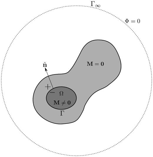
Schematic diagram of an unbounded domain with a fictitious boundary Γ∞ on which the magnetic potential vanishes, Φ = 0. The unbounded domain contains an unmagnetized region where |$\mathbf {M}=\mathbf {0}$| , and a magnetized region, Ω, where |$\mathbf {M}\ne \mathbf {0}$|. The magnetized region Ω has a boundary Γ with unit outward normal |$\hat{\mathbf {n}}$|, pointing from the inside of the region (−) to the outside of the region (+).
From hereon the approach is quite analogous to the approach of Gharti et al. (2018) for gravity anomalies problems, so we will be relatively brief, referring the reader to Gharti et al. (2018) for more detailed explanations of the method and its implementation.
2.2 Discretization
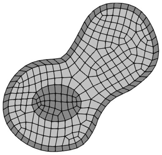
The unmagnetized region (light grey elements) and the magnetized region (interior dark grey elements) are discretized using spectral elements. A single layer of infinite elements is added outside the domain of interest to capture outer space (outer dark grey elements).
One key advantage of the SEM is that derivatives are directly computed on quadrature points, rendering this operation highly accurate. However, derivatives may be discontinuous across elemental boundaries, and therefore on such boundaries we average over all elements that touch a given node.
As described in detail in Gharti et al. (2018) within spectral elements we use GLL quadrature to construct the stiffness matrix, whereas in infinite elements we use Gauss–Radau quadrature in the infinite direction and GLL quadrature in other directions. Quadrature points on a spectral-infinite element interface coincide, thereby naturally coupling the two domains.
3 NUMERICAL EXAMPLES
We rely on MeshAssist (Gharti et al.2017) and Trelis/CUBIT (CUBIT 2017) for model preparation and meshing for all examples included in this paper. Each spectral element involves three GLL points in each direction, resulting in a total of 27 nodes per element. Our method is fully parallelized based on domain decomposition and the message passing interface. We use the mesh partitioning tool SCOTCH (Pellegrini & Roman 1996) to partition the mesh. We implemented parallel iterative Krylov solvers using PETSc, a portable and extensible toolkit for scientific computation (Balay et al.2015). We use a conjugate gradient solver with a geometric algebraic multigrid preconditioner (e.g. Stüben 2001) with a relative tolerance of 10−7. We have previously performed extensive convergence and strong scaling performance tests of our solver (Gharti et al.2018, 2019a).
3.1 Spherical magnetization
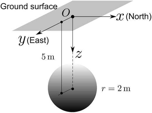
Model geometry for a spherical magnetization.
We created a model of size 40 m × 20 m × 12 m that covers the sphere and the observation points. For reasons of accuracy, we slightly extended the model above the ground surface to avoid placing the infinite element layer adjacent to observation points. We meshed the model using hexahedral elements. Initially, we selected an element size of 0.5 m inside the sphere and 1 m outside the sphere, as shown in Fig. 4 (left-hand panel). The mesh consists of 8576 elements and honours the sphere. We added an infinite-element layer outside the model surface based on a pole positioned at the centre of the sphere, as shown in Fig. 4 (right-hand panel). Opposite faces of infinite elements must be parallel or diverging with respect to the pole so that they do not converge at infinity. We performed four different simulations for the magnetized sphere located at four different latitudes. Simulations were run on a single processor and took about 40 s for each simulation. The analytical expression for the magnetic induction due to a sphere is given by eq. (A1).
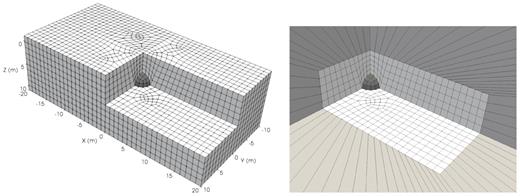
Left-hand panel: spectral-element mesh for a spherical magnetization. Right-hand panel: infinite elements radiating from the outer surface of the model (outer grey). The model is sectioned to visualize one quadrant of the magnetized sphere (dark grey). Only infinite elements from the visible outer surfaces are shown for clarity.
Fig. 5 shows total-field anomaly profiles calculated at the ground surface, z = 0, along the x-axis from −20 to 20 m. The computed result is in good agreement with the analytical solution, although we observe some discrepancies near the largest magnitudes. Both magnitude and direction of the total-field anomaly vary with the location of the magnetization. For the sphere located at latitudes, 0° and 90°, the total-field anomaly is symmetric about the centre of the sphere. The total-field anomaly is asymmetric about the centre of the sphere for other locations.
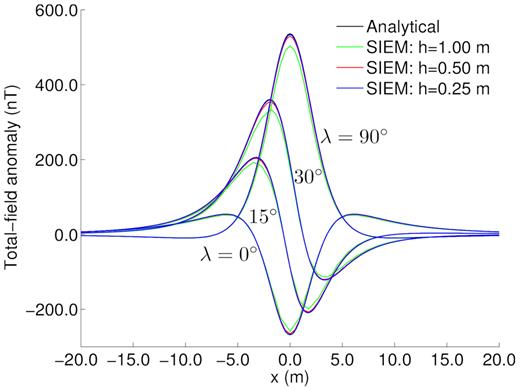
Profiles for the total field anomaly at z = 0 along the x-axis (North) for a spherical magnetization.
We refined the mesh by decreasing the element size to 0.25 and 0.5 m, respectively, inside and outside the dome, which increases the number of elements to 53 615. As shown in Fig. 5, the resulting total-field anomaly profile is very close to the analytical result, but we still observe some small discrepancies near the largest magnitudes. We further refined the mesh with element sizes of 0.125 and 0.25 m, respectively, inside and outside the dome, thereby increasing the total number of elements to 156 538. This refinement gives a nearly perfect match with the analytical solution. The spherical geometry poses a challenge for the mesher, because the coarser meshes fail to properly capture the spherical shape of the magnetization.
In Fig. 6, we plot the components of the magnetic induction computed on the ground surface of the model. As expected, we observe different patterns for each component depending on the location of the magnetized spheres. The figure also illustrates how the magnetic field gradually changes according to the angle of magnetic inclination. For magnetic inclinations of 0° and 90°, all three components are either symmetric or antisymmetric about the centre of the sphere. This is not the case for other locations. The magnetic field is stronger near the magnetized sphere and decays away from it.
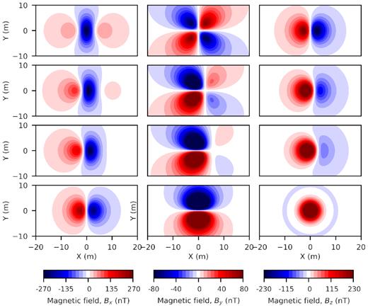
Magnetic field components (left-hand panel: Bx; middle: By; right-hand panel: Bz) plotted on the ground surface for a magnetized sphere located at latitudes 0°, 15°, 30° and 90° (top to bottom).
Finally, we plot the magnetic field lines on the vertical mid-plane, as shown in Fig. 7. It is interesting to see how the magnetic field lines emanate differently from the spheres for each location due to the different magnetic inclinations. These field lines explain the symmetry or asymmetry we observed for the total-field anomaly (Fig. 5).
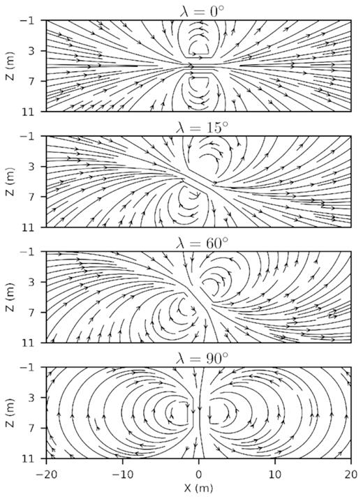
Magnetic field lines plotted on a mid-vertical plane for a magnetized sphere.
3.2 Rectangular prism
Next, we consider a rectangular prism of size 3 km × 4 km × 1 km with a magnetization strength M = 10 A m−1 located at a depth of 2.5 km from the ground surface, as shown in Fig. 8. The magnetization has an inclination of 30° and a declination of 0°. We created a model of size 28 km × 16 km × 8 km, which sufficiently covers the prism and the observation points. We extended the model slightly above the ground surface to avoid placing the infinite-element layer adjacent to observation points.
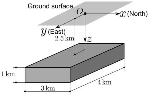
Model geometry for a magnetized rectangular prism.
Initially, we selected a coarse element size of 1 km and meshed the model using hexahedral elements. The mesh consists of only 4176 elements and honours the prism, as shown in Fig. 9. A single layer of infinite elements was added outside the mesh domain. We positioned the pole for the decay function required by the infinite elements at the centre of the prism.
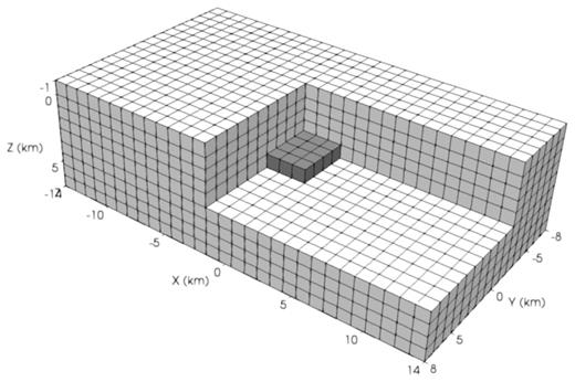
Left-hand panel: spectral-element mesh of a model with a buried rectangular prism. The model is sectioned to visualize the prism (dark grey).
An analytical expression for the total-field anomaly of a prism is given by eq. (A5). Fig. 10 shows a total-field anomaly profile computed at the ground surface, z = 0. We observe good agreement with the analytical result. Although we used a very coarse mesh, we obtain acceptable results because the mesh perfectly honours the prism.
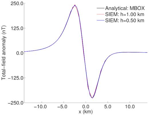
Profile for the total field anomaly at z = 0 for a rectangular prism.
Next, we refined the mesh by decreasing the element size from 1 to 0.5 km. The refinement increases the number of elements to 33 408. The resulting profile for the total-field anomaly is in excellent agreement with the analytical solution, demonstrating rapid convergence in terms of mesh refinement.
In Fig. 11, we plot the components of the magnetic induction computed on the ground surface. Due to the magnetic inclination, the magnetic field is not symmetric. It is stronger near the magnetized prism and decays ways from the prism.
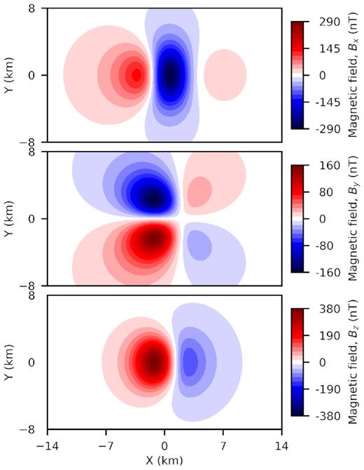
Magnetic field components (Top: Bx; Middle: By; Bottom: Bz) plotted on the ground surface for a rectangular prism.
Finally, we plot the magnetic field lines on the mid-vertical plane as shown in Fig. 12. The magnetic field lines emanate from and converge at the magnetic source at 30°, that is, the angle of inclination.
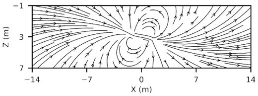
Magnetic field lines plotted on the mid-vertical plane for a rectangular prism.
3.3 Multiple spheres with varying size and magnetization
In this section, we design a problem similar to the example discussed in Gharti et al. (2018) and Martin et al. (2017) for gravity anomalies. We consider 100 spheres with varying radii and magnetization strengths organized in a vertical plane, as shown in Fig. 13. The model consists of 10 horizontally equidistant lines in the vertical plane with a vertical spacing of 10 km. Each horizontal line consists of 10 equidistant spheres with a horizontal spacing of 14 km. The lth horizontal line has a constant sphere radius, rl, and magnetization strength, M, determined by the relations, |$r_l=2+0.2\, (l-1)$| and |$M=1.5\, l$| A m−1, respectively, such that lines |$l=1\, \mathrm{to}\, 10$| are numbered top to bottom. The first sphere in the first horizontal line is located at x = 40 km, y = 0 km and z = − 5 km from the origin. We set the magnetic inclination and declination to 35° and 10°, respectively, for all spheres.
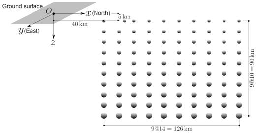
Layout of an array of 100 spheres of varying size.
We created a model of size 206 km × 80 km × 170 km covering all spheres and observation points. The outer surfaces of the model lie 40 km in each direction from the nearest sphere centre. We selected an element size of |$0.2\, r_\mathrm{ s}$| inside a sphere and |$0.4\, r_\mathrm{ s}$| outside a sphere, where rs is the sphere’s radius. This approach gradually coarsens the mesh from top to bottom, varying the element size inside the sphere from 0.4 to 0.76 km and outside the sphere from 0.8 to 1.52 km. This strategy ensures the same number of elements in all spheres (Fig. 14). Although not strictly necessary, this maintains a relatively uniform resolution for all spheres. The mesh consists of 2 886 000 spectral elements for a total of 22 808 007 degrees of freedom. We used 160 processors, on which it took about 7 min to compute the magnetic field. We set the magnetic inclination and declination of the regional field to 35° and 10°, respectively.
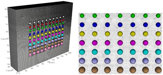
Left-hand panel: spectral-element mesh for an ensemble of 100 spheres. Mesh elements on the spheres are not shown for clarity. Right-hand panel: zoom in on a frontal view of the mesh. Spheres with the same colour have the same magnetic properties.
As a benchmark, we computed the total-field anomaly using MBOX (Blakely 1995). MBOX divides the model into a number of rectangular prisms. Each subprism uses the analytical solution given in eq. (A5) and the total-field anomaly is given by the superposition of the contributions of all the subprisms. We discretized the model using uniform cubic cells. Since the smallest spectral element has a size of 0.4 km and each spectral element has three GLL points in each direction, we chose a cubic cell of size 0.2 km. Consequently, the MBOX grid resolution is similar to the finest region of the spectral-element mesh, and hence the MBOX model is sampled more finely than the spectral-element model. There are a total of 1 611 488 cells with non-zero magnetization. We set 293 observation points each at two elevations, namely, 0 and 25 km, along the x-axis, resulting in a total of 586 observation points. The calculations took about 45 min on a single processor. Since the computational cost for the MBOX solution is proportional to the number of observation points for a given discretization, the total computational cost for the 22 808 007 points, that is, the total number of points in the spectral-element mesh, would be huge. On the other hand, the total computational cost for the SIEM is independent of the number of observation points for a given discretization.
We plot total-field anomaly profiles at two elevations along the x-axis, specifically at 0 and 25 km, as shown in Fig. 15. For both profiles, we observe excellent agreement of the SIEM and the MBOX solutions, with the analytical solution given by eq. (A3). At zero elevation, we clearly observe the influence of individual spheres as indicated by peaks and troughs. Magnitude of the peaks decreases and that of the troughs increases along x, that is, North direction due to the magnetic inclination. At far away from the sphere ensemble, that is, elevation 25 km, individual influences diminish and all spheres behave as a single entity as indicated by a smooth curve.
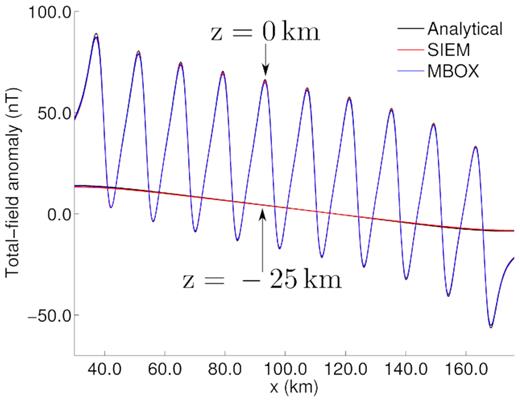
Total-field anomaly profiles at elevations of z = 0 km and z = −25 km for an ensemble of spheres.
In Fig. 16, we plot the components of the magnetic field on the ground surface. We clearly observe the influence of each column of magnetized spheres. Although the spheres are symmetrically placed about the x-axis, the magnetic field is not symmetric due to the inclination and declination.
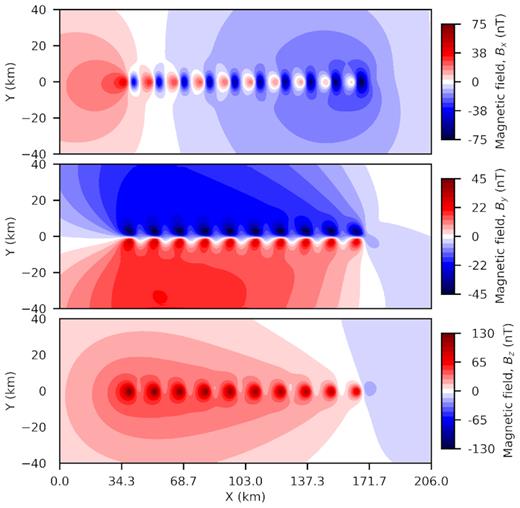
Magnetic field components (Top: Bx; Middle: By; Bottom: Bz) plotted on the ground surface for an array of magnetic spheres.
Finally, we plot magnetic filed lines on the mid-vertical planes through the sphere centres, as shown in Fig. 17. We observe the complicated interactions of the magnetic fields contributed by the individual spheres. Outside the spheres ensemble, magnetic field lines are regular as the individual influence of the spheres diminishes.

Magnetic field lines plotted on the mid-vertical plane for an array of magnetic spheres.
3.4 Application to an underground ore mine
To demonstrate our method for realistic 3-D problems, we compute the magnetic field for an existing underground ore mine, namely, the Pyhäsalmi mine in Finland. This active, deep mine contains massive sulphide deposits with copper and zinc ore bodies (Puustjärvi 1999). The complete mine layout and surrounding infrastructure are shown in Fig. 18 (left-hand panel). For more details on the mine and its microseismic event characteristics, see Oye et al. (2005). Fig. 18 (right-hand panel) shows the 622 m × 622 m × 622 m 3-D mine model, which consists of host rock, ore body and stopes, that is, mined-out cavities. Due to the mine’s complex geometry, it is a very challenging problem to calculate the magnetic field. We assume uniform magnetization within the ore body with a magnetization strength of 20 A m−1, a magnetic inclination of 75° and an declination of 10°.
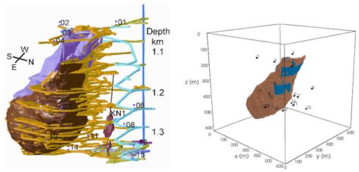
Left-hand panel: Pyhäsalmi mine with surrounding infrastructure: copper/zinc ore body (brown/pink), access tunnels (yellow), elevator shaft (dark blue) and seismic stations (numbered). The passage for quarried ore is labelled KN1. Right-hand panel: 3-D model of the Pyhäsalmi mine: stopes (blue) and ore body (brown). The remainder is host rock. Geophones are indicated by black dots and numbered.
We meshed the model using an average element size of 10 m. Due to the complex geometry, actual element sizes may differ in some areas, as shown in Fig. 19. The mesh involves 294 500 spectral elements and 2 517 769 degrees of freedom. We used 80 processors for the parallel simulation which took about 1 min.
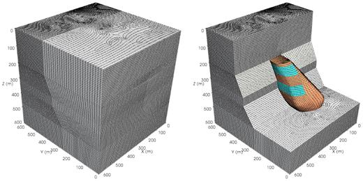
Left-hand panel: spectral-element mesh for the Pyhäsalmi mine model. Right-hand panel: interior section of the mesh visualizing the ore body (brown) and stopes (cyan).
Fig. 20 shows the components of the magnetic field computed on the top surface, that is, at z = 0 m.
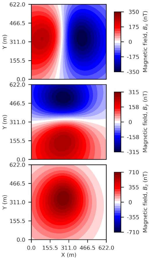
Magnetic field components (Top: Bx; Middle: By; Bottom: Bz) plotted on the ground surface for an ore mine.
Additionally, we plot magnetic field lines on the mid-vertical plane, as shown in Fig. 21. Imprints of cavities are observed in the field lines.
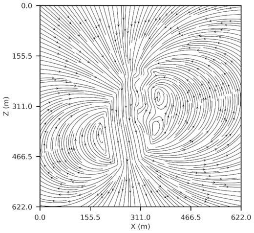
Magnetic field lines plotted on the mid-vertical plane for an ore mine.
Finally, we also compute the total-field anomaly on the top surface and compare with the MBOX solution, as shown in Fig. 22. For the MBOX simulation we use a cell size of 3.8875 m. There are a total of 25 921 observation points on the top surface. Since only the ore body is magnetized, there are only 149 739 non-zero cells. The MBOX calculation takes about 2 hr 42 min to run on a single processor to compute the total-field anomaly at 25 921 observation points. This is significantly larger than the SIEM, which takes only 1 min to run on 80 processors for 2 517 769 observation points. Since MBOX’s computational cost is proportional to the number of observation points, the total computational time would be huge if we had to compute the solution for all 2 517 769 observation points
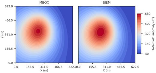
Total-field anomaly plotted on the ground surface for an ore mine. (Left-hand panel) MBOX. (Right-hand panel) SIEM.
The total-field anomaly computed by the SIEM and MBOX are very similar in pattern, but the magnitude of the MBOX total-field anomaly is less than the SIEM. The cubic cells used for the MBOX solution are unable to accurately capture the complex shape of the ore body and generally underestimate the surface area or the volume of complicated 3-D objects.
4 CONCLUSIONS
We have successfully implemented an SIEM to solve the unbounded Poisson/Laplace equation for magnetic anomalies induced by magnetized objects. We benchmarked our results with analytical solutions and the MBOX package (Blakely 1995) for a range of problems and used the Pyhäsalmi mine as a practical 3-D example.
Our tests show that the method is highly accurate and efficient. Since there is only a single layer of infinite elements, the additional computational cost associated with ‘outer space’ is insignificant. The computational cost is independent of the number of observation points. Consequently, the method is very efficient for large-scale problems. For additional performance improvement, GPU acceleration will be of future interest.
Inversion of magnetic data is also a future interest, in particular, the planetary magnetic fields (Holme & Bloxham 1996; Lewis & Simons 2012; Plattner & Simons 2017). The main advantage of our numerical discretization of the unbounded Poisson equation is that it can be naturally coupled with the laws of continuum mechanics that govern geostatic and geodynamic deformation.
ACKNOWLEDGEMENTS
We thank Volker Oye, Katja Sahala and ISS for access to the mine model. We thank Frederik J. Simons for helpful discussions which inspired this work and important feedback on this manuscript. Parallel programs were run on computers provided by the Princeton Institute for Computational Science and Engineering (PICSciE). 3-D data were visualized using the open-source parallel visualization software ParaView/VTK (www.paraview.org). 2-D snapshots were created using the open-source Python plotting library Matplotlib (www.matplotlib.org). Most of the model sketches were created using the open-source vector graphics editor Inkscape (inkscape.org). This research was partially supported by NSF grants 1644826 and 1550901. Our software is open source and freely available via the Computational Infrastructure for Geodynamics (CIG; geodynamics.org). We thank Editor Prof. Richard Holme, Alain Plattner and an anonymous reviewer for their insightful comments which helped to improve the manuscript.
REFERENCES
APPENDIX A: ANALYTICAL SOLUTIONS
In this section, we list all analytical solutions used in our benchmarks. In what follows, depth z is positive downwards.
A1 Dipole or sphere
A2 Multiple spheres
A3 Semi-infinite rectangular prism
We may compute the total-field anomaly for a rectangular prism of thickness h by evaluating eq. (A5) twice. The total-field anomaly for this case is equal to the total-field anomaly evaluated for z1 minus the total-field anomaly evaluated for z1 = z1 + h.
