


SUMMARY
A new method is proposed to estimate separately 3-D heterogeneities of intrinsic and scattering attenuation parameters of seismic shear waves. The method, which assumes isotropic scattering, consists of two steps. First, the source, site and mean path (both intrinsic and scattering attenuations) terms are estimated by an envelope-fitting method for each earthquake event; second, these attenuation parameters are mapped to 3-D space in a tomographic manner by using sensitivity kernels of the attenuation parameters. Monte Carlo simulation is adopted to take account of the effect of the depth-dependent velocity structure in the envelope calculation. The proposed method was then applied in southwestern Japan. The result showed that both intrinsic and scattering attenuations were stronger in the Kyushu region, where tectonic activity was higher than in other studied regions. This association of attenuation parameters with tectonic activity is consistent with previous findings. The proposed method thus provides an alternative to multiple lapse time window analysis, a widely used method for separately estimating intrinsic and scattering attenuation factors.
1 INTRODUCTION
Seismic attenuation in frequency ranges higher than 1 Hz is often classified into intrinsic and scattering attenuations (e.g. Sato et al.2012). Although both types of attenuation result in decreased seismic wave amplitudes at seismic stations, the attenuation mechanism differs between them. Intrinsic attenuation is caused by energy absorption processes in the medium. In contrast, wave scattering due to random heterogeneities of the Earth’s velocity structure excites coda waves, and the distribution of direct wave energy to the coda causes observed wave amplitudes to become small. To characterize the Earth medium, intrinsic and scattering attenuations should be separately estimated.
Radiative transfer theory is widely used to model coda excitation. Initially, isotropic scattering was assumed (Wu 1985; Zeng et al.1991), but later the theory was extended to treat various scattering phenomena, including non-isotropic scattering processes (Sato 1995) and scattering with phase conversion (Zeng 1993; Margerin et al.2000). Many previous studies (e.g. Padhy et al.2007; Jing et al.2014; Wang & Shearer 2017) have separately estimated intrinsic and scattering attenuations by envelope fitting based on radiative transfer theory. The Qopen software package, developed by Eulenfeld & Wegler (2016), can be used to estimate not only attenuation parameters but also source amplitude and site amplification terms. In addition, multiple lapse time window analysis (MLTWA; Fehler et al.1992; Hoshiba 1993) is widely used for simultaneous estimation of attenuation parameters.
After simultaneous estimation of intrinsic and scattering attenuations, the next challenge is to estimate the heterogeneous distribution of attenuation parameters. Carcolé & Sato (2010) used MLTWA to estimate intrinsic and scattering attenuations at individual Hi-net stations (Okada et al.2004) and then interpolated between stations to derive the detailed 2-D distribution of attenuation parameters in Japan. Eulenfeld & Wegler (2017) derived the 2-D distribution of attenuation parameters in the United States by applying Qopen to USArray network data, followed by careful interpolation. Prudencio et al. (2013) proposed a spatial-weighting function for mapping intrinsic and scattering attenuation parameters in 2-D space. However, a method for estimating 3-D heterogeneity is still needed. Recently, Takeuchi (2016) successfully calculated sensitivity kernels for intrinsic and scattering attenuation parameters by a Monte Carlo simulation (e.g. Gusev & Abubakirov 1987; Yoshimoto 2000) based on radiative transfer theory. The sensitivity kernels derived by Takeuchi (2016) are essentially approximations of ones derived analytically (Mayor et al.2014; Margerin et al.2016), but the approximation approaches the analytical solution as the number of energy particles used in the simulation increases. One advantage of the approach used by Takeuchi (2016) is that it can be used to derive 3-D sensitivity kernels with a heterogeneous velocity structure. In this study, a new method for mapping attenuation parameters in 3-D space is proposed. The method consists of two steps. First, both intrinsic and scattering attenuation parameters, as well as source and site amplification terms, are estimated for each earthquake by an envelope-fitting method (Eulenfield & Wegler 2016). Then, the estimated attenuation parameters are mapped in 3-D space by using the envelopes synthesized in the first step and sensitivity kernels derived as proposed by Takeuchi (2016).
Wave scattering results in not only coda excitation but also broadening of the direct wave envelope. Envelope broadening has been modelled by radiative transfer theory using non-isotropic scattering coefficients estimated by a Born approximation (e.g. Hoshiba 1995; Przybilla et al., 2006, 2009; Wegler et al.2006) and by a Markov approximation method (Sato 1989; Saito et al.2002; Sawazaki et al.2011; Emoto et al.2012). Takahashi et al. (2009) estimated random velocity fluctuations in 3-D space from envelope broadening, and Takahashi (2012) estimated 3-D attenuation structures from the maximum amplitudes of direct S waves corrected for the effect of envelope broadening. The results presented here complement the structural information inferred by Takahashi and his colleagues, thus furthering our understanding of the Earth’s structure.
2 METHOD
2.1 Step 1: estimating source, site and path terms for individual earthquakes
First, the source, site and intrinsic and scattering attenuation factors are estimated simultaneously for individual earthquakes. Only S waves and isotropic SS scattering are considered here, and scattering attenuation is characterized by scattering coefficients. Although a non-isotropic scattering model is required to model the seismogram envelope of direct waves (e.g. Wegler et al.2006), it is still practical to use an isotropic scattering model to model coda waves (e.g. Zeng 2017). Gaebler et al. (2015) applied both acoustic and elastic radiative transfer theories to analyse the seismogram envelopes observed at the West Bohemia/Vogtland region, the border of the Czech Republic and Germany. They carefully compared the estimated attenuation parameters (intrinsic attenuation and mean-free path) by both isotropic and non-isotropic scattering models, and concluded that the intrinsic attenuation factors and transport (momentum transfer) scattering coefficients (e.g. chapter 4 of Sato et al.2012), which equals total scattering coefficients of the isotropic scattering model, estimated by both scattering models were almost the same. Hence, the isotropic scattering model would be applicable to the non-isotropic scattering medium with the use of transport scattering coefficients.
To avoid a trade-off between the source and site amplification terms, the geometrical mean of site amplification is assumed to be equal to one, although other constraints to avoid this trade-off would be acceptable. If scattering coefficient, |${{{g}}_{{i}}}{{(f)}}$|, is assumed, then |${{E(}}{{{g}}_{{i}}}{{(f),}}{\mathbf{{x}}_{{j}}}{{,t)}}$| can be calculated. If a sufficient number of observed data |${{W}}_{{{ij}}}^{{\rm{OBS}}}{{(t;f)}}$| are used, then the system of equations, eqs (2) and (3), becomes overdetermined and can be solved by the least-squares method for the |${\rm{\mathit{ N}\ + \ 2}}$| unknown parameters. As indicated by Eulenfeld & Wegler (2016), to avoid a trade-off between the intrinsic attenuation factor and the scattering coefficient, the system of equations should include the averaged amplitude of the direct S-wave term. Thus, by conducting a forward search for |${{{g}}_{{i}}}{{(f)}}$|, the |${\rm{\mathit{ N}\ + \ 3}}$| unknown parameters in eq. (1) can be estimated for the |${{i}}$|th earthquake. Note that correction for interevent differences in |${{{W}}_{{i}}}( {{f}} )$| and |${{{R}}_{{{ij}}}}{{(f)}}$| is necessary for these values to be compared between different events.
2.2 Step 2: mapping intrinsic and scattering attenuation parameters in 3-D space
Next, the intrinsic attenuation factors and scattering coefficients estimated in step 1 are mapped in 3-D space in a tomographic manner by using sensitivity kernels. In seismic tomography, differences between observations and calculations (traveltimes, waveforms, etc.) are utilized together with their sensitivity kernels to modify structural parameters (e.g. Nolet 2008). In this study, the envelopes synthesized in step 1 are used as observations. Because these synthesized envelopes should represent the estimated intrinsic attenuation factors and scattering coefficients, step 2 is regarded as a procedure for mapping the structural parameters estimated in step 1. In addition, because isotropic scattering is assumed, the calculated envelope shape should never coincide with the shape of the direct wave part of the observed envelope. By using the envelopes synthesized in step 1 as observations, therefore, the full information from the observations, including the direct wave parts, can be utilized, thus avoiding a trade-off between the intrinsic attenuation factor and the scattering coefficient.
3 APPLICATION IN SOUTHWESTERN JAPAN
The method was applied to data for 422 earthquakes recorded by 238 Hi-net stations in four regions of southwestern Japan (Kinki, Chugoku, Shikoku and Kyushu); a 1-D velocity structure based on the JMA2001 velocity model (Ueno et al.2002) was assumed (Fig. 1). The crustal part of this velocity structure is a good approximation of the 2-D velocity structure derived by active source seismic experiments conducted in the Chugoku and Shikoku regions (Ito et al.2009). Note that the relationship between isotropic and non-isotropic scattering models through transport scattering coefficients would hold in the homogeneous velocity medium (Gaebler et al.2015). The relationship between both scattering models with the depth-dependent velocity structure should be investigated, however, it is out of the scope of this paper. Some relationships between both scattering models are assumed to exist in the medium having a depth-dependent velocity structure. Nevertheless, scattering coefficients estimated in this paper would represent the scattering property of the medium. The earthquake magnitudes ranged from 3.0 to 4.5 on the Japan Meteorological Agency (JMA) scale; these magnitudes are sufficiently small for the effect of the source time function on the envelope to be neglected. In both steps 1 and 2, seismograms recorded at stations at epicentral distances of less than 100 km were used. A 1–2 Hz bandpass filter was applied to each seismogram, and then the mean square envelope was obtained by calculating the vector sum of the three-component seismograms. In eqs (1) and (4), |${{f}}$| was set to 1.5 Hz. In eq. (1), the attenuation parameters were assumed to be homogeneous for each earthquake. Higher frequency (shorter wavelength) seismograms sample narrower regions of the medium than lower frequency seismograms with longer wavelength; thus, the assumption of homogeneous attenuation parameters for each earthquake is more appropriate at the relatively low frequency of 1.5 Hz. Each envelope was smoothed by applying the moving average within a time window of 2 s, and then resampling every 1 s. Irrelevant envelopes, that is, ones due to contamination by another small earthquake or sensor calibration signal or ones reflecting sensor malfunctions, were excluded by visual inspection. As a result, the total number of envelopes used was 10 721. The Green’s functions in both steps 1 and 2 were calculated by a Monte Carlo simulation. 5 million particles were used in step 1 and 12 million particles in step 2. The azimuthal symmetry assumed in step 1 made it possible to reduce the number of particles used in step 1.
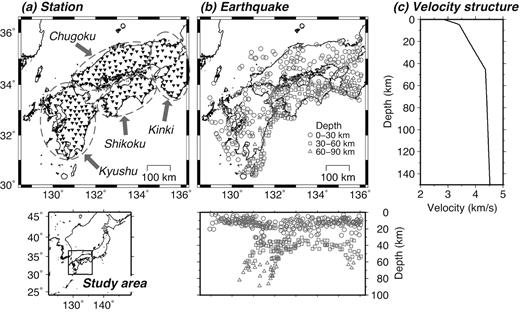
(a) Stations, (b) earthquake hypocentral distribution and (c) 1-D S-wave velocity structure (Ueno et al.2002) used in this study. The dash-lined ellipses in panel (a) indicate approximately the Kinki, Chugoku, Shikoku and Kyushu regions.
In step 1, because residuals were unimodal with respect to |${{{g}}_{{i}}}$| for all events, a golden section search for |${g}_{i}$| ranging from 0.001 to 0.1 km–1 was conducted. The time window for calculation of direct wave amplitudes was set to 10 s, starting from the theoretical arrival time of the direct S waves calculated with the JMA2001 velocity model (Ueno et al.2002). The coda time window was set to 40 s and immediately followed the direct wave window. Because the velocity structure (Fig. 1c) does not consider discontinuities such as the Moho, refracted and reflected waves were not modelled by the Green’s function |${{E(}}{{{g}}_{{i}}}{{(f),}}{{\mathbf{x}}_{{j}}}{{,t)}}$| of eq. (1). However, the observed amplitudes in the direct S-wave time window were averaged and the direct wave envelope shape was not used. In addition, long coda time window was used so that it would reflect the mean scattering characteristics of the medium. Hence, the effects of transient signals, that is, refracted or reflected waves, were expected to be small in both the direct S-wave and coda time windows.
Figs 2(a) and (b) show the estimated intrinsic attenuation factors and scattering coefficients for each earthquake, which were calculated in step 1. The errors of the inverse of the intrinsic attenuation factor |${{Q}}_{{i}}^{{\rm{ - 1}}}$| and the scattering coefficient |${{{g}}_{{i}}}$| for the event with the largest residuals were estimated by the jackknife test (e.g. Efron & Stein 1981) to be |${\rm{3}}{\rm{.33\ \times 1}}{{\rm{0}}^{{\rm{ - 3}}}}$| and |${\rm{1}}{\rm{.39\ \times 1}}{{\rm{0}}^{{\rm{ - 3}}}}$| km–1, respectively. Errors for other events were expected to be of about the same order as these values. For earthquakes that occurred in and around Kyushu, |${{Q}}_{{i}}^{{\rm{ - 1}}}$| ranged from about 0.008 to 0.009 and |${{{g}}_{{i}}}$| ranged from about 0.01 to 0.025 km–1, whereas in other regions |${{Q}}_{{i}}^{{\rm{ - 1}}}$| ranged from about 0.004 to 0.007 and |${{{g}}_{{i}}}$| was less than 0.005 km–1. These results, which imply that both intrinsic and scattering attenuations were larger in Kyushu than in the other regions, are consistent with previous findings (Hoshiba 1993; Carcolé & Sato 2010). The envelopes synthesized in step 1 agreed well with the observed envelopes (Fig. 2c).
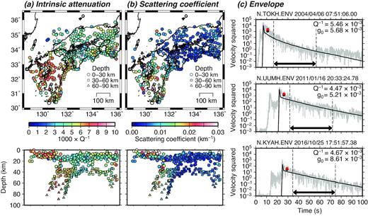
Estimated (a) inverse of the intrinsic attenuation factor |${{Q}}_{{i}}^{{\rm{ - 1}}}$| and (b) scattering coefficient |${{{g}}_{{i}}}$| for each earthquake and (c) comparison between observed envelopes (grey) and envelopes synthesized in step 1 (black). In panel (c), the double-headed arrows denote the coda time window used for calculating residuals, and the red and black dots denote the averaged amplitudes in the direct wave time window of the observed and synthesized envelopes, respectively.
In step 2, the time window was set to 50 s, starting from the theoretical S-wave arrival in each envelope. The resulting number of observations was 536 050. The attenuation structure was considered in the geographic region from 125.1°E to 138.7°E in the longitudinal direction, 27.5°N to 38.7°N in the latitudinal direction and from 0 to 150 km depth. The 3-D region was discretized into blocks, each of which measured 0.4° in both the longitudinal and latitudinal directions and 20 km vertically, except the vertical dimension of the blocks in the shallowest layer was 10 km. Because ARTB was applied to each earthquake sequentially, for each application, matrix |${\mathbf{G}}$| needed to include only those components related to a single earthquake. Hence, the calculation region of the sensitivity kernels was limited to a 3-D region that included the epicentre of the earthquake and those stations. The 3-D region was a rectangular shape with the epicentre at the centre of the square. A maximum horizontal extent of the region was about 6° in both latitudinal and longitudinal directions and the maximum depth was 150 km. Because each block size was 0.4° × 0.4° × 10 km for the shallowest layer and 0.4° × 0.4° × 20 km for other layers, the size of matrix |${\mathbf{G}}$| for each earthquake was then about |$[({\rm{15\ \times \ 15\ \times \ 8\ \times \ 2)\ \times \ 1000}}$|] to |$[({\rm{15\ \times \ 15\ \times \ 8\ \times \ 2)\ \times \ 1500}}$|]: the first factor corresponds to the region used for sensitivity kernels calculation with two unknown parameters and the second factor corresponds to the data from 20 to 30 stations within the 50 s time window. The initial structural parameters were set as |${{{Q}}^{{\rm{ - 1}}}}{\rm{\ = \ 6}}{\rm{.67\ \times 1}}{{\rm{0}}^{{\rm{ - 3}}}}$| and |${{{g}}_{\rm{0}}}{\rm{\ = \ 0}}{\rm{.005}}$| km–1. These values approximately represented the attenuation structure of the Kinki, Chugoku and Shikoku region (Figs 2a and b). In ARTB, a priori variances are assigned to the data and model to stabilize the inversion. Because in eq. (4), the sensitivity kernels for the perturbed scattering coefficients tend to be smaller than those for the inverse of the intrinsic attenuation factors, a priori variances of the scattering coefficients were set to twice those of the inverse of the intrinsic attenuation factors. Even when a priori variances are set for the data and structural parameters, however, the resultant parameter perturbations may lead to structural parameters that are physically inappropriate, that is, |${{{Q}}^{{\rm{ - 1}}}}$| or |${{{g}}_{\rm{0}}}$| may have negative values. In such a situation, |${{{Q}}^{{\rm{ - 1}}}}$| or |${{{g}}_{\rm{0}}}$| must be small, so any structural parameters with negative values were replaced with |${\rm{0}}{\rm{.67\ \times 1}}{{\rm{0}}^{{\rm{ - 3}}}}$| for |${{{Q}}^{{\rm{ - 1}}}}$| and |${\rm{0}}{\rm{.0005}}$| km–1 for |${{{g}}_{\rm{0}}}$| before the inversion by ARTB was continued. Inversion was calculated only once in step 2 because the squared sum of the differences between the envelopes synthesized in step 1 and those calculated using the estimated structure converged after all earthquakes used. The overall features of the intrinsic attenuation factors and scattering coefficients estimated in step 1 (Figs 2a and b) were reproduced by the 3-D distribution derived in step 2 (Figs 3 and 4). From the checkerboard resolution test results (see Section 4), values along the section shown in Fig. 4 are inferred to be reliable to depths up to 50 km whereas in other regions values are reliable only to depths up to 30 km.
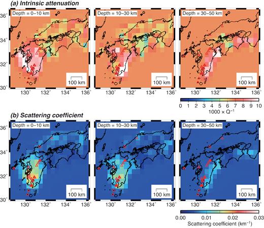
Estimated 3-D distributions of the (a) inverse of the intrinsic attenuation factor |${{{Q}}^{{\rm{ - 1}}}}$| and (b) scattering coefficient |${{{g}}_{\rm{0}}}$| obtained in step 2. Left-hand panels show the first layer (0–10 km depth), centre panels show the second layer (10–30 km) and right-hand panels show the third layer (30–50 km). Red triangles denote active volcanoes listed in the Japan Meteorological Agency (2013) catalogue.
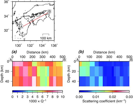
Distribution in vertical cross-section of the (a) inverse of the intrinsic attenuation factor |${{{Q}}^{{\rm{ - 1}}}}$| and (b) scattering coefficient |${{{g}}_{\rm{0}}}$| along line A–B shown in the map inset.
4 DISCUSSION
A checkerboard resolution test was conducted to check the reliability of the step 2 result. In this test, the source and site amplification factors were assumed to be fully known, and the assumed checkerboard pattern was |${{{Q}}^{{\rm{ - 1}}}}{\rm{ = \ 6}}{\rm{.70\ \times 1}}{{\rm{0}}^{{\rm{ - 3}}}}{\rm{ \pm 3}}{\rm{.00\ \times 1}}{{\rm{0}}^{{\rm{ - 3}}}}$| and |${{{g}}_{\rm{0}}}{\rm{ = \ 0}}{\rm{.010\ \pm \ 0}}{\rm{.005}}$| km−1. In the checkerboard test results (Fig. 5), the assumed structural anomaly patterns and amplitudes of both the intrinsic attenuation factors and scattering coefficients were well retrieved for blocks in the shallowest and second layers beneath the land areas (Fig. 5, left-hand side and centre). In the third layer, the checkerboard pattern was retrieved only beneath the Shikoku region, where the hypocentral distribution was the densest. The regions where the checkerboard pattern was well retrieved correspond to those where the step 2 inversion result was reliable (Fig. 5). In addition, the jackknife test (Efron & Stein 1981) was used to estimate the errors of the structural parameter values shown in Fig. 3. The data set for the 422 earthquakes was divided into 10 subsets, each of which included about 40 earthquakes without duplication. Then the same mapping procedure was applied to the data without each subset, and the estimation errors of each block were calculated using the results. The resulting estimation errors for the intrinsic attenuation factors and scattering coefficients are shown in Fig. 6. The maximum errors were |${\rm{5}}{\rm{.28\ \times 1}}{{\rm{0}}^{{\rm{ - 3}}}}$| for |${{{Q}}^{{\rm{ - 1}}}}$| and |${\rm{6}}{\rm{.03\ \times 1}}{{\rm{0}}^{{\rm{ - 3}}}}$| for |${{{g}}_{\rm{0}}}$|.
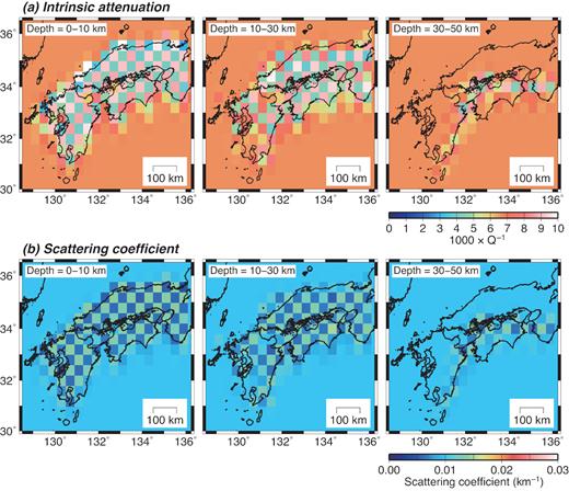
Estimated 3-D distributions of the (a) inverse of the intrinsic attenuation factor and (b) scattering coefficient in the checkerboard resolution test results.
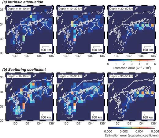
Estimated 3-D distributions of the errors for the (a) inverse of the intrinsic attenuation factor and (b) scattering coefficient by the jackknife test.
The strong intrinsic attenuation regions in the first layer (Fig. 3a, left-hand side) showed strong correlations with the regions with low S-wave velocity at 2 km depth estimated by Nishida et al. (2008). Because in a sedimentary basin, regions of low velocity correlate with regions with strong total attenuation (e.g. Lawrence & Prieto 2011), the presence of a low S-wave velocity in the shallow layer of southwestern Japan can explain in part the strong intrinsic attenuation seen in Fig. 3(a). In addition, in the Kyushu region, the complex stress field (e.g. Matsumoto et al.2015) and the presence of active volcanoes, especially in central and southern Kyushu, would result in strong intrinsic attenuation. Strong scattering regions (|${{{g}}_{\rm{0}}} \approx {\rm{0}}{\rm{.01}}$| km−1) in the shallowest layer corresponded to the locations of active volcanoes, reflecting the heterogeneities caused by the presence of magma and hydrothermal systems beneath the volcanoes. In central Shikoku, both intrinsic and scattering attenuations were low in the second and third layers (Figs 3 and 4). This low attenuation region is consistent with the distribution of the total attenuation factors in that region estimated by Kita & Matsubara (2016). Further, along the section through the Kyushu and Shikoku regions (Fig. 4), the depth dependency of intrinsic attenuation and scattering coefficient seems to differ between the northeastern and southwestern parts of this low attenuation region. The derived attenuation structure may relate to the slow-earthquake activities and non-volcanic tremors that occur in this region (e.g. Beroza & Ide 2011), although further investigation is needed to examine this relationship in detail.
Previous studies have shown that intrinsic attenuation factors and scattering coefficients are frequency-dependent (e.g. Nakamura et al.2006; Carcolé & Sato 2010). To examine the frequency dependency of these parameters, the same mapping method was applied to seismogram envelopes in the frequency range of 4–8 Hz. |${{f}}$| in eq. (4) was set to 6 Hz. The result showed that both intrinsic attenuation and scattering were stronger in the Kyushu region than in the other regions (Fig. 7), similar to the results for the 1–2 Hz frequency band (Fig. 3). However, the distributions of intrinsic attenuation factors and scattering coefficients were apparently patchier in the higher frequency range, probably because the higher frequency seismograms sampled smaller regions than lower frequency seismograms. Nevertheless, both |${{{Q}}^{{\rm{ - 1}}}}$| and |${{{g}}_{\rm{0}}}$| values were obviously smaller in the 4–8 Hz frequency range than in the 1–2 Hz range. This result suggests that the frequency dependency of intrinsic attenuation and scattering coefficients in these regions should be further studied.

In this study, because scattering was assumed to be isotropic, observed envelopes were not used in step 2. However, the formulations of both Eulenfeld & Wegler (2016) and Takeuchi (2016) would hold in a non-isotropic scattering medium, and a non-isotropic scattering model is required to explain the direct wave envelope (e.g. Sato et al.2012). Hence, extending the proposed method to deal with non-isotropic scattering would allow observed envelopes to be utilized in step 2 and make the estimated structure more reliable. In addition, the assumption in step 1 of homogeneity with respect to both intrinsic and scattering attenuations determines the resolution of heterogeneous structures. This resolution could be enhanced by considering the path dependency of structural parameters in step 1.
5 CONCLUSION
A new two-step method was proposed for the separate estimation of intrinsic and scattering attenuation parameters in 3-D space. In the first step, the source, site amplification, and intrinsic and scattering attenuation parameters are estimated simultaneously for each earthquake by an envelope-fitting method. Then, in the second step, the attenuation parameters of each earthquake are back-projected into 3-D space by sequential adjustment of the structural parameters in a tomographic manner. In both steps, a Monte Carlo simulation is used with a 1-D velocity structure to calculate seismogram envelopes. In the second step, sensitivity kernels of the structural parameters are used along with a 1-D velocity structure. When this method was applied to seismogram envelopes recorded in southwestern Japan, the retrieved structure showed larger intrinsic and scattering attenuations in the Kyushu region than in the other regions, reflecting differences in tectonic settings among the regions.
ACKNOWLEDGEMENTS
MO used waveform data from Hi-net, which is operated by the National Research Institute for Earth Science and Disaster Resilience, Japan. All waveforms used in this study can be downloaded from the Hi-net website (http://www.hinet.bosai.go.jp/?LANG=en, last accessed June 2018). MO referred to the unified earthquake catalogue produced by the JMA in cooperation with the Ministry of Education, Culture, Sports, Science and Technology of Japan. The catalogue can be downloaded from the JMA website (http://www.data.jma.go.jp/svd/eqev/data/bulletin/index_e.html, last accessed June 2018). MO thank the editor Joerg Renner and the reviewers, Ulrich Wegler and an anonymous reviewer, for their constructive comments. MO also thank Tatsuhiko Saito for helpful discussions. This work was partly supported by the Cooperative Research Programs of the Earthquake Research Institute of the University of Tokyo and JSPS KAKENHI, Grant Numbers JP17H02064 and JP18K13622.
