


SUMMARY
A detailed and precise knowledge of ocean bottom topography is essential in many geoscientific and oceanographic applications. Shipborne echo sounding provides the only direct bathymetric method. However, even after decades of applying this technique only a fraction of the global ocean could be covered. Alternatively, gravity data inversion is a feasible method to infer ocean bottom topography since the gravity field correlates with topography at short to medium wavelengths. Gravity field observables are globally provided by dedicated satellite missions like GOCE, GRACE and GRACE-FO and, over the oceans, by satellite altimetry. Regional and local measurements are realised by means of ground-based, shipborne and airborne gravimetry. For the first time in Europe a jet aircraft was used for airborne gravimetry. During the GEOHALO flight campaign over Italy and the Tyrrhenian, Ionian and Adriatic seas in June 2012, the German research aircraft HALO carried an entire suite of geodetic-geophysical instrumentation, including gravity metres. The careful processing of the gravity data acquired by the CHEKAN-AM instrument of the German Research Centre for Geosciences allowed to achieve an accuracy at the mGal level. Subsequently, the Parker–Oldenburg inversion was applied to predict ocean bottom topography along the GEOHALO profiles flown over the ocean. To constrain the parameter space in the inversion we used the Crust1.0 model. Finally, the obtained results were compared to the General Bathymetric Chart of the Oceans in order to estimate the performance of the method. Our study demonstrates that airborne gravimetry aboard a jet aircraft is capable to provide valuable data for regional geoscientific studies.
1 INTRODUCTION
A sound knowledge of the topography is essential in most geoscientific studies. While continental topography is determined by direct methods and with high resolution, the situation is more complicated for ocean bottom topography. Shipborne echo sounding provides the best method in bathymetry. However, this method is extremely time consuming, so that the majority of the Earth’s ocean is still only sparsely mapped (Weatherall et al.2015). In the latest release of the global data set GEBCO_2014 only 18 per cent of all grid cells are constrained by shipborne echo soundings (Weatherall et al.2015). Utilizing the gravity field signal forms another possibility to infer ocean bottom topography. The exterior gravity field of the Earth is captured by a number of methods, namely, globally by satellite gravimetry and satellite altimetry, and regionally and locally by terrestrial, airborne and shipborne campaigns. The gravity field highly correlates with topography at short to medium wavelengths (30–300 km; Talwani et al.1972; Watts 1978). A large number of studies make use of this relationship to infer ocean bottom topography by dedicated inversion methods (e.g. Dixon et al.1983; Calmant 1994; Smith & Sandwell 1994; Watts et al.2006; Becker et al.2009; Weatherall et al.2015). In this study we applied a calculation scheme based on the Parker–Oldenburg inversion (Parker 1973; Oldenburg 1974). This method has been successfully adopted in other studies, for example, Schaller et al. (2015) who used terrestrial gravity data in the Central Andes to invert for depths of the Mohorovičić discontinuity (Moho), and Steffen et al. (2017) who inferred Moho depths from EIGEN-6C4 data in Greenland. Here, we will present inversion results using gravity data obtained during the GEOHALO campaign.
2 GEOHALO
GEOHALO was an airborne mission carried out in June 2012 using the German ‘High Altitude and Long Range Research Aircraft’ (HALO). This aircraft is based on a Gulfstream G550 business jet that was modified to accommodate a large variety of instrumentation for atmospheric and Earth system research. Since GEOHALO was the first dedicated geoscientific HALO mission and it was the first time in Europe that a jet aircraft was utilized for aerogravimetry, the study area was chosen for its extensive geoscientific database, which enabled to demonstrate HALO’s feasibility for airborne geodesy and geophysics. The mission was flown over Italy and the adjacent Tyrrhenian, Adriatic and Ionian seas. The entire Mediterranean, especially the region under investigation, is characterized by a complex tectonic pattern (see Section 3) and, therefore, subject to an increased geohazard. It was an additional goal of GEOHALO to apply airborne gravity and magnetic measurements to enhance the knowledge of the potential fields. Also, these results can be used to provide further constraints for the investigation of the lithospheric structure and plate kinematics.
The mission was carried out on four days in June 2012 comprising 16 500 profile kilometres at eight parallel north–south profiles and four crossing lines (see Fig. 1). GEOHALO was flown at an average altitude of 3500 m and with a mean flight velocity of 425 km/h. A ninth profile (the easternmost dashed cyan profile) was flown at an altitude of 10 000 m following exactly the previous lower profile (westernmost red profile). The flights at the high altitude as well as at occasionally larger flight velocities of 600 km/h (especially along the tie lines) helped to check the performance of the instruments. GEOHALO comprised an entire suite of airborne geodetic-geophysical instrumentation. Besides two spring-type gravimeters, namely CHEKAN-AM (Elektropribor, Russia) and KSS-32M (Bodenseewerke, Germany), HALO was equipped with two vector and two scalar magnetometers, a laser altimeter, GNSS antennas and receivers for positioning and for reflectometry/spectrometry, and different inertial navigation systems (INS). For the first time the successful realization of GNSS reflectometry aboard a jet aircraft could prove to resolve sea-surface topography (SST) anomalies with respect to the geoid (Semmling et al.2014). Likewise, airborne laser altimetry was applied at such large altitudes to effectively retrieve SST (Henkel 2014). Results of GEOHALO airborne gravimetry were discussed by Petrovic et al. (2015), Barzaghi et al. (2015) and Lu et al. (2017), and are now used in this study.

3 GEOLOGY AND TECTONIC SITUATION
Gravity anomalies reflect density anomalies which are related to the geological and tectonic situation. The gravity effect of a heterogeneous density structure might overlie the usually much stronger gravity effect of the topography at medium wavelengths. Therefore, a sound knowledge of the geology and tectonic setting in the area of investigation is essential for the interpretation of resulting gravity anomalies and subsurface models.
The present-day tectonic situation in the Mediterranean evolved from the interplay between the African and Eurasian plates and further microplates. As a result various subduction zones and the remnants of older subduction zones with all their characteristic density changes are present within the study area. Carminati & Doglioni (2005) gave a thorough overview of the tectonic situation, which has been adopted for Fig. 2 with an inset of the study area. The most prominent feature is the convergent plate boundary between the African and Eurasian continental plates denoted by the red line.
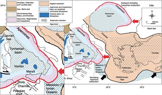
Present geodynamic framework adapted from Carminati & Doglioni (2005). The red line corresponds to the present day subduction zone separating the African and the Eurasian continental plates. The composition of the Tyrrhenian Sea is mostly uniform, with two small patches of oceanic crust. The Adriatic (east of Italy) and Ionian (south of Italy) seas display heterogeneous composition due to the crossing of the subduction zone through these areas. The inset on the left-hand side shows the study area of the GEOHALO mission. The exact position of the plate boundary is still under debate (see the text and Fig. 7).
In this area most of the crust is of continental composition with the uppermost parts being dominated by sediments due to old and recent input derived from erosion of the surrounding mainland (Carminati & Doglioni 2005). Also, during the Messinian eustatic lowstand the Mediterranean dried up several times which produced thick sequences of evaporites in the basins. Due to the repetitive removal of the water a significant isostatic rebound occurred, especially in the Ionian and central Tyrrhenian seas (Carminati & Doglioni 2005). The Tyrrhenian basin is mainly of uniform composition with two small patches of oceanic backarc lithosphere. The Ionian and Adriatic seas (see also Fig. 1) display a more complex situation because the subduction zone is crossing through these areas, with corresponding changes in composition. The (few) profiles flown over the Adriatic Sea during the GEOHALO campaign cross the plate boundary. In the Ionian Sea the exact position of the plate boundary is still under debate (Carminati & Doglioni 2005; Jenny et al.2006; Bennett et al.2008; Carminati et al.2012; Neri et al.2012). In Fig. 7 the plate boundary is plotted after Carminati et al. (2012). All subsequent interpretations are based on this study. Hence, in the Ionian Sea the flight profiles are all situated to the north of the plate boundary.
4 THEORETICAL BACKGROUND
4.1 Parker–Oldenburg inversion
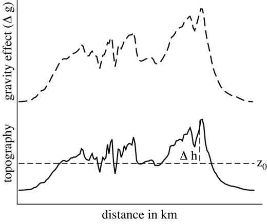
Schematic sketch of the POI scheme. The |$\Delta h(\vec{r})$| represents the topographic heights with respect to a constant level at z0 (thin dashed line). The solid line denotes the interface between two media of constant density (water/air and crystalline crust/sediments). The upper dashed line corresponds to the gravity effect of this layer.
4.2 Filtering
Since the POI includes a downward continuation it is unstable at very short wavelengths. Also, the resolution of the gravity data may be limited due to preceding processing steps (Section 5.1). At long wavelengths the topography tends to be isostatically compensated. Even more, subducting plates and composition changes within lower crustal layers also cause a long-wavelength signal which should be eliminated. Therefore, this long-wavelength signal part of the ocean bottom topography cannot be obtained by POI. These reasons motivate to applying a bandpass filter whose optimal parameters have to be identified in the inversion process. The long-wavelength part of the signal has to be taken from another source of information, for example, independent observational or model data. Here, we made use of the General Bathymetric Chart of the Oceans (GEBCO; Weatherall et al.2015). To comply with the filtering applied with the POI, the GEBCO data have to be low-pass filtered whereby the filter characteristic has to be consistent to the POI bandpass filter. The resulting low-pass filtered GEBCO data are then added to the POI results.
|$\mbox{and} \, \, \, \lambda _1 \gt \lambda _2 \gt \lambda _3 \gt \lambda _4$|.
|$\mbox{where} \, \, \, \lambda _1 \gt \lambda _2$| are the limiting wavelengths. Both transfer functions are shown in Fig. 4.
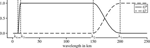
Transfer functions of the filters defined in eqs (2) and (3). Solid line: bandpass filter, thick dashed line: low-pass filter. The determining wavelengths λ1–λ4 are marked from right to left.
5 DATA PROCESSING
5.1 Gravity disturbances from GEOHALO airborne gravimetry
The gravity data used in this study were acquired during the GEOHALO campaign (Section 2) using the sea–air gravimeter CHEKAN-AM of GFZ Potsdam (Lu et al.2017). In order to derive absolute gravity values from the raw data several processing steps had to be realized. For a detailed description of the principles of airborne gravimetry one may refer, for example, to Forsberg & Olesen (2010).
The accuracy of the inferred gravity disturbances is estimated to be 3 mGal (with |$1\, \mbox{mGal}=\mbox{10}^{-5}\,\,\mbox{m}/\mbox{s}^{2}$|). A thorough validation of the final gravity solution was done comparing the GEOHALO gravity disturbances with synthetic data predicted by the EIGEN-6C4 global gravity field model (Förste et al.2014) and ground data of the Italian gravity database. The resulting RMS values confirmed the accuracy to be at the 3 mGal level (see also Fig. 5). On the other hand this validation led to the identification of errors in the Italian gravity database (Barzaghi et al.2015).

Processing of the raw gravity data. Green line: the raw CHEKAN gravity data after filtering, Eötvös correction and reduction of normal gravity (without correction for aeroplane acceleration). Orange line: vertical acceleration derived from differentiating (filtered) velocities calculated from GNSS Doppler measurements. Blue line: difference between raw gravity data (green line) and GNSS inferred kinematic acceleration (orange line), that is, gravity disturbance at flight altitude. Red line: EIGEN-6C4 (Förste et al.2014) gravity disturbances predicted at flight altitude (|$1\, \mbox{mGal}=\mbox{10}^{-5}\,\,\mbox{m}/\mbox{s}^{2}$|).
Since the POI incorporates FFT, the gravity data need to be referenced to a mean altitude and interpolated to equally spaced points along the respective profile. The differences of the actual flight altitude w.r.t. a mean altitude are small (mean difference 12 m, maximum difference 64 m). Therefore, we simply used the vertical gradient of normal gravity to pointwise continue the gravity data to the mean altitude. The error of this continuation stays at the sub-mGal-level and, thus, below the error level. Furthermore, the gravity data were extended at both profile start and end using gravity disturbances predicted by EIGEN-6C4 (Förste et al.2014). This step facilitates the subsequent filtering and Fourier transform in such a way that effects of discretization and limited length of the data series were minimized. The latter refers to the handling of the leakage problem. Before transforming the data into the frequency domain a Tukey window was applied where the filter width equals the length of the extended profile such that the signal content remains undamped along the original extension of the profile. The gravity disturbances at each extended profile were then reduced by its respective mean. This will not change the result since the long wavelengths are filtered off anyway.
5.2 POI processing scheme
The extended and mean-value reduced gravity disturbance profile can now be introduced into the POI (Section 4). The gravity disturbances comply best with Parker’s definition of the gravity effect Δg since they are defined as radial derivatives of the disturbing potential T, and the potential of the material layer can be regarded as a residual (i.e. small or disturbing) potential as well. Anyway, any remaining constant or long-wavelength offset will be filtered off when applying the bandpass filter. The average depth to the ocean bottom, the density contrast of the two layers and the filter wavelengths are those parameters which are essential for the performance of the POI. In order to select reasonable starting values we made use of the global crustal model Crust1.0 (Laske et al.2013). For each profile an average density value ρc and the mean value of depth z0 were obtained. The lower cut-off wavelength of the bandpass filter was set to roughly half the profile length. The upper cut-off wavelength was set concurring with the filter parameter used in the processing of the gravity data (Section 5.1). Distinguishing between the three ocean regions for each profile the chosen parameter values are given in Tables 1–3, Section 6. Due to the characteristic of the POI and the necessary filtering, the result has a bandpass limited spectrum (see Section 4). Therefore, the long-wavelength part is obtained from the low-pass filtered GEBCO model (Weatherall et al.2015) and added to the POI result. The parameters of the low-pass filter were set according to the bandpass filter parameters of the respective profile (see Fig. 4). The resulting ocean bottom topography is then compared to the GEBCO data using the RMS of the differences as measure for the fit. The entire calculation scheme is applied separately to each profile. The results are given and discussed in Section 6.
Tyrrhenian Sea: table of chosen parameters (crustal density (ρcrust), average depth (z0) and bandpass filter (BPF) wavelengths). See Fig. 7 for profile locations and Fig. 8 for the resulting topography of the respective profile. The last column gives the RMS of the differences between the calculation results and the GEBCO data.
| Profile | |$\mathbf {\rho _{crust}}$| | z0 | BPF | RMS | |||
|---|---|---|---|---|---|---|---|
| |$\mathbf{{in\,kg}/{m}^{3}}$| | in m | wavelengths in km | in m | ||||
| T1 | 1930 | 2800 | 150 | 100 | 18 | 6 | 525 |
| T2 | 1930 | 1500 | 100 | 50 | 18 | 6 | 202 |
| T3 | 1900 | 1700 | 100 | 50 | 18 | 6 | 309 |
| T4 | 1930 | 1800 | 150 | 100 | 18 | 6 | 552 |
| T5 | 1930 | 1200 | 150 | 100 | 18 | 6 | 369 |
| T6 | 1930 | 900 | 75 | 50 | 18 | 6 | 167 |
| T7 | 1930 | 900 | 75 | 50 | 18 | 6 | 251 |
| T8 | 1930 | 100 | 75 | 50 | 18 | 6 | 548 |
| T9 | 1930 | 100 | 75 | 50 | 18 | 6 | 228 |
| T10 | 1820 | 100 | 75 | 50 | 18 | 6 | 385 |
In order to review the reliability of the GEBCO data for the assessment of the results, the data source in the study area was checked. Most of the data in Europe, and thus in the study area, are taken from EMODnet (Marine Information Service 2016). These data in turn were based on numerous campaigns with shipborne echo soundings. Only small data gaps remain. Therefore, it can be assumed that the GEBCO data are suitable for the validation of the results.
5.3 Effect of different parameter values
First, we will discuss the influence of the different parameters on the POI results in general. For that, one example profile was selected and the results for two different values of each parameter are shown in Fig. 6. Note that the given results in this figure do not include the final calculation step of adding the long wavelengths. The results of changes in the upper cut-off wavelength of the bandpass filter (GB) are displayed in Figs 6(a) and (b). The changes for different filter wavelengths are small. The difference between bandpass-filtered GEBCO (green line) and POI result rises with increasing upper cut-off wavelength. In general, the upper cut-off wavelength depends on the length of the profile. Also, one should pay attention to the isostatic situation of the study area (see also Section 1).
![Results of POI for varying upper cut-off filter wavelengths (a and b), density (c and d) and mean depth z0 (e and f). The respective parameter is given above each subplot. The filter wavelength λ1 stands for [λ1λ2λ3λ4] = (a) [120 70 18 6] km, (b) [300 200 18 6] km. In each subplot the orange line corresponds to the POI result, the thin green line denotes the topography data from GEBCO and the thick blue line gives the bandpass-filtered GEBCO data.](https://oup.silverchair-cdn.com/oup/backfile/Content_public/Journal/gji/216/2/10.1093_gji_ggy456/1/m_ggy456fig6.jpeg?Expires=1750353691&Signature=pLK9AWClqzpYhBnZJfdiLYTWNR8V-7lCtZXb371jTCWCu1k2-sMQCLKt6niYu-h1~PqsYQ-wnOmojlpzOSKe1EMKPCiodsdIxyu8BH4eoj7IqboC4G47nPjKFAijIz80fof2~a1yW7aByTN2hxY4hOsDo9CVJuuJM1kyv16R743k64qnWi~HrwMJQjeCHTUAgkpLGXwssohr2MWt4nIiF~GKMTWQzxq5M20UioLBhbWd68~-lwqCgAw3ddEzIaOAXUhshfsXIyfO9F0VFnIY1EPy4tU7sXANCUJU9cmW8FZPDJ0ZoQ9xaJk4Ll8f4GDwFd7pBk12mT0IITtOczYq8g__&Key-Pair-Id=APKAIE5G5CRDK6RD3PGA)
Results of POI for varying upper cut-off filter wavelengths (a and b), density (c and d) and mean depth z0 (e and f). The respective parameter is given above each subplot. The filter wavelength λ1 stands for [λ1λ2λ3λ4] = (a) [120 70 18 6] km, (b) [300 200 18 6] km. In each subplot the orange line corresponds to the POI result, the thin green line denotes the topography data from GEBCO and the thick blue line gives the bandpass-filtered GEBCO data.
The POI results depend strongly on changes of the crustal density ρc (see Figs 6c and d). A high density contrast leads to small amplitudes in the resulting topography and vice versa. This can be explained easily by potential theory. Under the condition that the average depth to the interface is constant, a body having higher mass relative to its surroundings causes a higher gravity value/local gravity maximum. Thus, in order to explain larger gravity values, a higher density or a larger volume is required. A larger volume corresponds to undulations of higher amplitude in the topography. Therefore, if the density (of the lower layer) is set to smaller values, the resulting amplitudes of the inverted topography are higher. If the density is set to higher values, the amplitudes of the resulting topography are lower.
In Figs 6(e) and (f), the results for a varying mean depth z0 are displayed. Here, the amplitudes of the results increase with increasing depth. This can also be explained by potential theory. The gravity effect of a mass decreases with increasing distance. Therefore, if the average depth (z0) is set to larger values, a larger volume, hence higher amplitudes of the topography are required to explain the gravity signal. Thus, the z0 acts diametrically to the density, but its influence is not as strong.
Hence, a number of different models with either higher density and larger average depth or lower density and smaller depth can be found resulting in a similar level of fit. Therefore, it is important to constrain the parameter range by additional data.
6 RESULTS
In Fig. 7 the location of all profiles is given. The parameters chosen for the inversion together with the RMS of the differences between the resulting and the GEBCO data are given in Tables 1–3. The results for the entire calculation procedure are given in Figs 8–10.
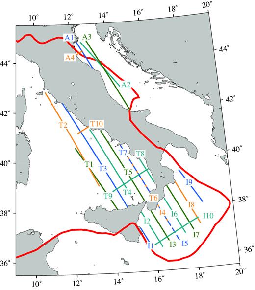
Overview of all profiles in the Tyrrhenian Sea (T1 to T10), the Ionian Sea (I1 to I10) and the Adriatic Sea (A1–A4). The thick red line denotes the plate boundary taken from Carminati et al. (2012).
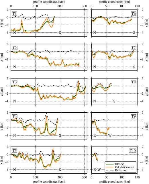
Results for the Tyrrhenian Sea (orange line) compared to GEBCO model (green line) and the difference between the two (black dashed line).
6.1 Tyrrhenian Sea
The ocean bottom topography results for all profiles in the Tyrrhenian Sea are displayed in Fig. 8. The orange line represents the results of the complete calculation scheme, the green line displays GEBCO data, while the black dashed line denotes the difference between the two. Parameters concurring with these results are given in Table 1. In Fig. 8 the long-wavelength part of the ocean bottom topography was added. Also, the plots are limited in length to the area of the original profiles.
In the Tyrrhenian Sea all profiles cover an area of stretched continental lithosphere, except for two patches of oceanic lithosphere (Carminati & Doglioni 2005). These patches are small compared to the length of most profiles and, therefore, do not overly influence the results.
In Crust1.0 the density is 1930 kg/m3 for the uppermost layer on most profiles. In the northern part the density is slightly lower. Therefore, a crustal density of 1930 kg/m3 was assigned to almost all profiles while for profile T10 a density of 1820 kg/m3 was set. The average depth (z0) varies strongly, from large depths in the central Tyrrhenian Sea to zero at the coast.
As shown in Fig. 8 the resulting topography fits very well with the GEBCO data. The RMS of the differences is between 160 and 550 m compared to profile lengths of up to 300 km and depth values of ≤ 4 km. At some profiles the amplitudes of local maxima are too large compared to the GEBCO data. As discussed in Section 5.3 this hints at densities that are too small and/or average depths that are too high. The profiles T1–T5 have lengths of more than 200 km and are located above the central part of the Tyrrhenian Sea. In general, the fit is very good except for a few local maxima that display larger amplitudes in the calculation results, mainly at the southern end of T1, T3 and T5. On profiles T3, T4 (partly) and T5 just north of the coastline of Sicily and southern Italy, a small rise of ≈ 2 km amplitude is visible. On all profiles in this area the gravity signal is sensitive to this rise, thus leading to large amplitudes in the profile-wise inversion results.
Profiles T6 and T7 were flown at the same ground track but at different altitudes (T6 at 10 500 m and T7 at 3 500m). Still, the resulting topography fits very well to the GEBCO data in both cases with a slightly lower RMS for T6 compared to T7. It should be noted that T6 even displays the lowest RMS of all profiles in the Tyrrhenian Sea. Thus, this proves again the suitability of a high flying jet aircraft for these kind of studies. At profile T8 larger discrepancies between calculation results and GEBCO are visible. Since this profile runs closest to the coast the discrepancies could be caused by the gravity effect of the nearby continental landmasses. Profile T9, the northernmost of the two east–west profiles, displays very good results. Especially the large topography gradient from east to west is reproduced well. T10 is rather short, especially compared to the resolution of the gravity data of 12 km. Still, the generally satisfying results are shown here for completeness.
6.2 Ionian Sea
The results for the Ionian Sea are given in Table 2 and displayed in Fig. 9. (See also to Fig. 7 for an overview of the locations of the profiles and the nearby plate boundary.) Additionally, from Fig. 2 it is evident that these profiles cross areas of changing composition. Profile I1 is running in parallel to the plate boundary (Carminati et al.2012) for its entire length. Still the fit is with an RMS of 525 m acceptable. Profiles I2, I3, I7 and I8 show good fits in the south, while large offsets are visible in the north. A uniformly good fit is evident for profiles I4, I5, I6 and I9. I4 and I5 are also situated at the same horizontal location. The east–west crossing profile I10 displays a good fit in the eastern part of the profile with larger discrepancies in the western part.
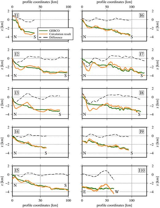
Results for the Ionian Sea (orange line) compared to GEBCO model (green line) and the difference between the two (black dashed line).
Ionian Sea: table of chosen parameters (crustal density (ρcrust), average depth (z0) and bandpass filter (BPF) wavelengths). See Fig. 7 for profile locations and Fig. 9 for the resulting topography of the respective profile. The last column gives the RMS of the differences between the calculation results and the GEBCO data.
| Profile | |$\mathbf {\rho _{crust}}$| | z0 | BPF | RMS | |||
|---|---|---|---|---|---|---|---|
| |$\mathbf{{in\,kg}/{m}^{3}}$| | in m | wavelengths in km | in m | ||||
| I1 | 1930 | 1500 | 75 | 50 | 18 | 6 | 497 |
| I2 | 1930 | 2300 | 75 | 50 | 18 | 6 | 435 |
| I3 | 1930 | 2300 | 75 | 50 | 18 | 6 | 509 |
| I4 | 1930 | 2300 | 75 | 50 | 18 | 6 | 193 |
| I5 | 1930 | 2300 | 75 | 50 | 18 | 6 | 248 |
| I6 | 1930 | 2300 | 75 | 50 | 18 | 6 | 196 |
| I7 | 1930 | 2700 | 150 | 100 | 18 | 6 | 671 |
| I8 | 1930 | 2000 | 150 | 100 | 18 | 6 | 609 |
| I9 | 1930 | 1900 | 75 | 50 | 18 | 6 | 214 |
| I10 | 1930 | 2800 | 75 | 50 | 18 | 6 | 500 |
In general the fit of the inverted topography to the GEBCO data is sufficient in the southern part of the profiles but rather low in the north. Two explanations for the discrepancies are possible. First, it could be that the density varies significantly from north to south. As discussed before, the exact location of the plate boundary is still debated. If it was situated further to the north, it would cross the GEOHALO profiles, hence explaining the north–south changes in the fit. Second, there might be residual effects because a topographic correction was not applied to the gravity data (see Section 5.1).
6.3 Adriatic Sea
The results for the Adriatic Sea are given in Table 3 and are displayed in Fig. 10. In general, the topography in the Adriatic Sea is extremely flat. An inversion result of this type can be achieved with either very high densities or very small depths. In this case, the resulting small amplitudes are mainly due to the small average depths (z0) between 10 and 50 m. Still, the resulting amplitudes are too high compared to the GEBCO data. Here, the gravity signal of the sea floor topography is probably mixing with the gravity signal of a lower layer (e.g. between sediments and crystalline crust) which is likewise very close to the sea surface.
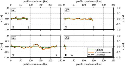
Results for the Adriatic Sea (orange line) compared to GEBCO model (green) and the difference between the two (black dashed line).
Adriatic Sea: Table of chosen parameters (crustal density (ρcrust), average depth (z0) and bandpass filter (BPF) wavelengths). See Fig. 7 for profile locations and Fig. 10 for the resulting topography of the respective profile. The last column gives the RMS of the differences between the calculation results and the GEBCO data.
| Profile | |$\mathbf {\rho _{crust}}$| | z0 | BPF | RMS | |||
|---|---|---|---|---|---|---|---|
| |$\mathbf{{in\,kg}/{m}^{3}}$| | in m | wavelengths in km | in m | ||||
| A1 | 2100 | 10 | 75 | 50 | 18 | 6 | 77 |
| A2 | 2000 | 50 | 75 | 50 | 18 | 6 | 41 |
| A3 | 1930 | 40 | 150 | 100 | 18 | 6 | 95 |
| A4 | 2100 | 10 | 100 | 50 | 18 | 6 | 203 |
6.4 Discussion of results
Discussing the results one has to keep in mind that one major goal of the GEOHALO campaign was to investigate whether it is feasible to utilize a jet aircraft for geoscientific research in general and especially for airborne gravimetry. Normally flown at much higher velocities (up to 900 km/h) the air speed adopted for GEOHALO was only about 425 km/h. Together with the necessary low-pass filtering this limits the along-track resolution (to 12 km in this case). A further distinctive capability of HALO is to fly at very high altitudes. The attenuation of the gravity field with altitude is known (due to upward continuation). However, there is a trade-off between flight altitude and speed in terms of the achievable resolution and economic efficiency w.r.t. the costs that have to be considered for future flight planning. Hence, it could be shown that for all flight profiles the measured gravity data coincide well with predictions by the recent global high-resolution gravity field model (EIGEN-6C4, see Section 5.1). Moreover, due to the long flight lines inconsistencies in the Italian gravity database could be recovered (Barzaghi et al.2015).
Generally, introducing GEOHALO airborne gravimetry data into the POI yields reasonably accurate results in areas with mostly homogeneous density distribution (Tyrrhenian Sea). In areas with strong changes in the density structure and/or thick sedimentary cover masking undulations of lower boundaries, the method is not easily applicable (Adriatic and Ionian seas) but could be used to invert for the next lower layer. In the Tyrrhenian and Ionian seas the RMS resulting from the comparison of the POI results with the GEBCO model was even lower for the data obtained at the higher altitude. This also proves that for regional studies the resolution of the gravity data measured aboard a jet aircraft is still high enough.
Studies using this kind of aircraft can add an intermediate part of the gravity field spectrum. The resolution of HALO airborne gravimetry is much higher than that of satellite-only models. Since the range of the jet aircraft is much higher than that of the smaller (unpressurized) aircraft the bandwidth of the measurable spectrum can considerably be increased. The long range also provides the possibility to connect areas that might be measured at higher resolution but being separated from each other, thus enabling to detect offsets and other differences.
7 SUMMARY AND OUTLOOK
The proposed calculation procedure is proven to be a useful tool to obtain ocean bottom topography. It is based on the inversion of gravity (Oldenburg 1974) and makes use of an iterative process. We compared the results with the GEBCO data set and were, thus, able to confirm the reliability of the results in the Tyrrhenian Sea. The situation is more complex in the Ionian and Adriatic seas, where the tectonic situation with the plate boundary between Eurasian and African plates as well as compositional changes related to remnants of older subduction (Carminati & Doglioni 2005; Carminati et al.2012) impeded the inversion process.
The gravity data used in this study were acquired by the HALO research aircraft as part of the GEOHALO mission in 2012. As was shown by this and previous publications (Scheinert 2013; Barzaghi et al.2015; Petrovic et al.2015), the gravity data measured on board the HALO aircraft are useful for a number of geoscientific applications. Larger flight altitude and higher flight velocities limit the resolution of the acquired data. Nevertheless, airborne gravimetry on board a jet aircraft is able to add an intermediate part of the gravity field spectrum to the observations, since it fills the gap between lower flying, smaller research aircraft and satellite observations. Also, HALO’s ability to cover large and remote areas is useful to study regions that could not be reached so far. Additionally, it is possible to connect existing smaller yet separate surveys to check the quality of their data.
However, one has to deal with the question of the limited resolution. The POI provides a bandpass limited result. In most cases the long-wavelength part of the spectrum can be obtained from a regional model with coarser resolution. The very short wavelengths, however, cannot be derived from gravity field modelling. In this study, the filtered inversion result coincides extremely well with the GEBCO data having a resolution of 30 arc-seconds. In most regional geoscientific studies the absence of very high frequencies will likewise not be a problem, just another factor to keep in mind when evaluating the results.
In future work a combined solution of the GEOHALO gravity data with a global model could serve as the basis for 3D gravity forward modelling. This model should of course incorporate all landmasses in the study area. The boundary between sediments and crystalline crust as well as different locations of the subduction zone can be modelled in this manner. Still, this work is beyond the scope of this publication.
The presented calculation procedure will be adapted to incorporate 2D modelling. It shall be adapted to regions where respective topographic information is sparse. This is especially the case for the subglacial topography in Antarctica. However, gravity data have to be combined with all available data (such as from ice-penetrating radar, seismics and geology). The Antarctic gravity anomaly grid (Scheinert et al.2016) together with recently acquired airborne gravimetry provide a sound basis to start such an investigation.
ACKNOWLEDGEMENTS
This investigation was supported by the German Research Foundation (DFG) in the frame of the Priority Program 1294 (Atmospheric and Earth system research with the ‘High Altitude and LOng Range Research Aircraft’; projects SCHE 1426/5-1 and KU 1207/8-1, SCHE 1426/17-1 and FO 771/8-1). We would like to thank the editor Richard Holme for handling our submission and the reviewer H.-J. Götze for his comments that helped to significantly improve this manuscript.
REFERENCES
