


SUMMARY
In this study, we discuss possible origins of the D″ reflector beneath the North Atlantic region based on a combined analysis of P and S wave data. We use over 700 USArray station recordings of the Mw 6.3 earthquake that occurred in April 2010 in Spain. In order to investigate the D″ layer we look for waves reflected off the top of it, namely PdP and SdS waves, and compare them to the core–mantle boundary (CMB) reflections used as reference phases. The differences in traveltimes and amplitudes are sensitive to D″ properties. Because the USArray installation generates a dense array, we are able to provide an almost continuous map of the detection or absence of PdP and SdS waves in the North Atlantic region. We use a Bayesian inversion for traveltimes, together with synthetic seismogram calculations, to find the best-fitting D″ properties, (Vp, Vs) jumps across the D″ interface and D″ thickness. We find that the best-fitting models are for a D″ layer of about 300 km thick, with or without a velocity gradient of about 30 km at the top of it. Regardless of the model type, positive and similar velocity increases in both P and S velocities at the D″ interface, ranging from 2.7 to 3.8 per cent, are required to fit the data well. Our data rule out velocity decreases in P and S waves at the D″ interface as well as no velocity reduction above the CMB. There are also regions where we do not observe PdP and SdS waves. Collectively, these observations suggest lateral variations in both chemistry and temperature, combined with phase transitions. For instance, ancient oceanic basalt debris from the Farallon slab could be modulating the detection of the D″ reflector in this region.
1 INTRODUCTION
The D″ layer (Bullen, 1949) marks the transition between the molten iron-rich outer core and the predominantly crystalline lower mantle, thus modulating the heat flux across the core–mantle boundary (CMB). The D″ layer therefore plays a central role in whole mantle convection processes (Lay 2007a), core convection, and geodynamo processes (e.g. Glatzmaier et al. 1999). Improved characterization of the D″ region should lead to a better understanding of whole mantle dynamics and geomagnetism. This layer is associated with a wide-range of seismic complexity and interpretations of this layer remain uncertain (see Wysession et al. 1998; Cobden et al. 2015, for reviews). Possible candidates for the generation of a reflector at the top of D″ range from solid–solid phase transitions, subducted slab debris, preferred alignment of anisotropic materials, thermochemical layering or a combination of these factors (Lay & Helmberger 1983; Sidorin et al. 1999; Hernlund & McNamara 2015). This discontinuity has often been associated in seismic studies with strongly positive S velocity jumps and weakly positive or negative P-wave velocity jumps (e.g. Hutko et al. 2008; Thomas et al. 2011; Cobden et al. 2013; Wysession et al. 1998; Cobden et al. 2015, for reviews) such that the preferred candidate to explain such a layer is a structural phase transition from MgSiO3 (or pyrolitic) bridgmanite (Br) to post-perovskite (pPv) within an isochemical lower mantle (Murakami et al. 2004; Oganov & Ono 2004). However, global seismic characterization of this layer, in combination with mineral physics results, suggest that such a Br-pPv transition in a pyrolitic mantle cannot reconcile all the seismic observations (e.g. Akber-Knutson et al. 2005; Grocholski et al. 2012; Cobden et al. 2015).
The global large-scale D″ velocity structures (i.e. larger than 1000 km) are mostly constrained by both P- and S-wave velocity tomographic models (Ritsema et al. 2011; French & Romanowicz 2014a; Moulik & Ekström 2014; Chang et al. 2015; Koelemeijer et al. 2016; Durand et al. 2017, 2016). Recently, using new normal mode cross-coupling data, Durand et al. (2016) show evidence for a more complex shear velocity pattern through the D″ region, characterized by stronger odd spherical harmonic degrees, in contrast to the well-known dominant degree 2 pattern (Dziewonski et al. 1993). This method reveals more heterogeneous large low-shear-velocity provinces with various local maxima, well correlated with some clusters of hotspot sources. Moreover, the global scale D″ mineralogy can be constrained by combining compressional and shear velocity tomographic models, assuming select mineral physics results (Mosca et al. 2012; Koelemeijer et al. 2016). For instance, by inverting for both global P- and S-wave velocity perturbations, Koelemeijer et al. (2016) show a negative correlation between the global shear wave and bulk sound velocity variations within D″, suggesting either the presence of pPv or large-scale chemical heterogeneities in the lowermost mantle, or a combination of these effects (Kennett & Widiyanto 1998; Masters et al. 2013).
Global tomography is, however, unable to resolve small-scale D″ heterogeneities (smaller than 1000 km) which makes it difficult to attribute the observed large scale velocity heterogeneities to any particular effect such as temperature, composition or mineral texture. To do this, regional high-resolution studies of D″ are required. D″ reflected waves, combined with core-reflected waves, are particularly useful, as they allow one to probe the reflector as well as velocity variations within the D″ region. D″ reflected waves have been reported in several different regions (e.g. Lay & Helmberger 1983; Davis & Weber 1990; Weber & Davis 1990; Weber & Körnig 1990; Young & Lay 1990; Houard & Nataf 1992, 1993; Weber 1993; Reasoner & Revenaugh 1999; Russel et al. 2001; Thomas & Kendall 2002; Lay et al. 2004b; Thomas et al. 2004a, b, 2015; Wallace & Thomas 2005; Avants et al. 2006; Lay et al. 2006; Kito et al. 2007; Hutko et al. 2008; Sun et al. 2008, 2016; Chaloner et al2009; Hutko et al. 2009; Yao et al. 2015). Many of these studies use either P- or S-wave observations. However, in order to advance our ability to interpret these observations in terms of thermochemical boundaries, phase transitions, and/or anisotropy, it is essential to obtain constraints on both wave types. To date, relatively few studies attempted to characterize the D″ layer using a combination of P- and S-wave data (e.g. Weber & Davis 1990; Weber 1993; Russel et al. 2001; Kito et al. 2007; Hutko et al. 2008, 2009; Chaloner et al2009; Thomas et al. 2011; Cobden et al. 2013).
In this study, we focus on characterizing D″ beneath the North Atlantic by combining unprecedented P and S data sets. The D″ layer beneath this region has been studied before (Weber & Körnig 1990, 1992; Houard & Nataf 1992; Krüger et al. 1995; Braña & Helffrich 2004; Wallace & Thomas 2005; Yao et al. 2015). These studies show the existence of a ∼200–300-km-thick D″ layer with P- and S-wave velocity perturbations of the order of 1–4 per cent—using either P-wave data (Weber & Körnig 1990, 1992; Houard & Nataf 1992; Krüger et al. 1995; Braña & Helffrich 2004) or S-wave data (Wallace & Thomas 2005; Yao et al. 2015). Except for Yao et al. (2015), most of these studies had limited coverage due to the limited number of earthquake-station combinations suitable to study the D″ structure in this area. In April 2010, a Mw 6.3 earthquake occurred in Spain that was recorded at the dense USArray (IRIS Transportable Array 2003), thus providing high-quality P- and S-wave recordings, enabling significant improvements on the coverage of this region. Yao et al. (2015) analysed this event using array processing techniques in order to study the D″ discontinuity, focusing only on shear wave signals. Here we combine P- and S-wave information to constrain the nature of D″ in this region. We use a Bayesian approach to invert for the characteristics of D″, combined with synthetic seismogram calculations. We show that this approach leads to tighter constraints on the sharpness and lateral variability of D″ beneath the North Atlantic region. In combination with existing mineral physics results, we discuss a few interpretations that involve lateral thermochemical variations.
2 DATA SELECTION AND PROCESSING
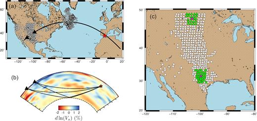
(a) Map of the selected data after the application of the SNR criterion. White triangles are the stations, the red star is the Mw 6.3 Spanish earthquake, April 2010, and grey diamonds are great-circle-path mid-points. The black thick line profile corresponds to the tomographic section shown in (b). (b) Section in SEISGLOB2 (Durand et al. 2017) tomographic model corresponding to the profile shown in (a) (black thick line). Superimposed are the paths of the core and D″ reflected waves for a distance from the earthquake of 70° and 80°. A fast region is observed at the base of the mantle around the reflection point of the core-reflected wave. (c) Examples of subarrays (green triangles) used to compute vespagrams. The pink triangle represents the starting station around which we look for at least 20 stations in a width of ±2°.
D″ reflected waves, PdP and SdS, can be difficult to detect in individual seismograms. We therefore stack seismograms in order to obtain a convincing signal that stands out from the noise level. To do so we apply seismic array methods and compute fourth-root vespagrams (Davis et al. 1971; Rost & Thomas 2002; Schweitzer et al. 2002); this approach is particularly powerful for detecting small amplitude signals such as PdP and SdS (e.g. Thomas et al. 2015). A vespagram is a signal processing method that computes the seismic energy that reaches an array for a given backazimuth and various horizontal slowness values; we generally assume that the wave propagates along the great-circle path and thus arrives with the theoretical backazimuth, however, we also test whether our waves travel out of plane using slowness-backazimuth analysis. We find that our recorded waves travel mostly on the great circle path.
For a good slowness resolution in the vespagram the aperture of the seismic array should be large enough such that arrivals between the stations are different, but small enough such that the plane wave approximation is valid and the waves are coherent across the array. Therefore, instead of computing a single vespagram for the entire data set, we form square subarrays of ±2° (see Fig. 1c) and compute a vespagram for every possible subarray. For this procedure we impose that the subarrays contain at least 20 stations, which ensures good quality vespagrams. We filter the data before stacking, using a Butterworth bandpass filter between 1 and 10 s for P-wave data and between 3 and 20 s for S-wave data to further enhance the quality of our observations. Our processing steps yield 428 P vespagrams and 438 S vespagrams (see Table 1) that can be used for further analysis.
3 TRAVELTIME MEASUREMENTS
In order to constrain D″ thickness and velocity structure, various wave combinations can be used. For instance, differential traveltimes of the direct waves (P or S) and the D″ reflected waves (PdP or SdS) have been used before and allow a precise estimation of D″ depth, since neither wave is affected by D″ velocities, which can affect PcP or ScS traveltimes (e.g. Chaloner et al2009; Yao et al. 2015). However, these differential traveltimes are also very sensitive to the mantle structures above D″ and are well-known to have a maximum of sensitivity at the turning point of the direct wave, usually ocurring around 1800–2300 km depth. Velocity structures located in this depth range can thus greatly affect the estimation of the D″ thickness. That is why we choose to use differential traveltime measurements between the D″ reflected wave and the core-reflected wave only, denoted δtPcP − PdP and δtScS − SdS. These differential traveltimes are well suited to focus on the D″ structure since the paths of both waves are very similar outside the D″ layer, which practically restrict their sensitivity to D″ (Lay et al. 2004b).
We thus inspect every vespagram in order to see whether any D″ reflected signals were present on both P and S vespagrams (Fig. 2). To that aim, we first use TauP (Crotwell et al. 1999) to predict slowness and traveltime of D″ reflected waves for D″ thicknesses varying from 100 to 500 km (dashed red curves in Fig. 2) and we then look for signals lying around this curve that have a signal-to-noise ratio greater than 10. When a D″ reflector can be detected (Figs 2b and d), we perform differential traveltime measurements δtPcP − PdP and δtScS − SdS. These first traveltime measurements are done by manual picking in the vespagrams. Examples of picked traveltimes are shown as red points in Fig. 2. Every picked wave was characterized by two lobes, one positive and one negative (see Fig. 2), so we decided to pick the traveltime in the middle of the waveforms when they have zero amplitude. In order to evaluate the uncertainties of the traveltime delays and the detection of the D″ reflected waves, we perform a boostrap analysis (e.g. Efron 1982) meaning that for every vespagram where D″ reflected waves have been detected we recompute 100 vespagrams by randomly resampling the subarray. Using the hand picked traveltimes to define a window where the D″ reflected wave is expected, we automatically pick traveltimes of PdP or SdS on the 100 bootstrap vespagrams. This leads to a distribution of traveltimes (Fig. 3) that we fit with a Gaussian function (see red curve in Fig. 3). The mean of the Gaussian, μ, gives a measure of the traveltime and its standard deviation, σ, the associated uncertainty. We keep the traveltime measurements obtained with the bootstrap analysis when at least 60 of the 100 measurements made on the bootstrap vespagrams lie within two standard deviations around the mean of the Gaussian distribution (see dashed lines in Fig. 3).
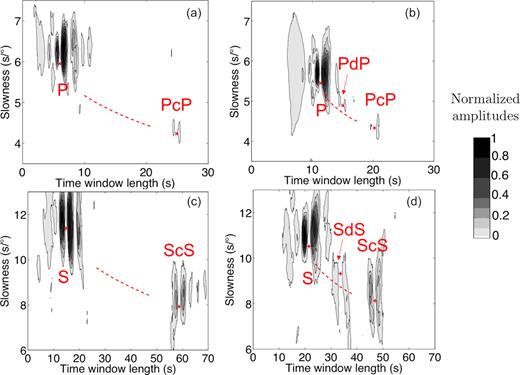
Examples of vespagrams for P (a, b) and S waves (c, d) computed for the groups of stations highlighted Fig. 1(c). Vespagrams in (a) and (c) correspond to the highlighted group of stations in the North in Fig. 1(c) and vespagrams in (b) and (d) correspond to the highlighted group of stations in the South in Fig. 1(c). They have been normalized to the maximum amplitudes and we highlight signals that have at least 2 per cent of the maximum amplitude. (a, c): Examples of vespagrams where the direct waves (P or S) and the core-reflected one (PcP and ScS) are detected. (b, d): Examples of vespagrams where D″ reflected waves (PdP and SdS) are detected. The red dashed curves are the predicted slownesses and traveltimes of D″ reflected waves for D″ thicknesses varying from 150 to 500 km.
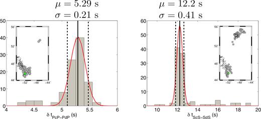
Example results of the bootstrap analysis performed for the same subarray as for the vespagrams shown Figs 2(b) (left) and d (right). Maps indicate the mid-point locations for these measurements (green symbols) within every performed measurement (grey symbols). We show the 100 traveltime measurements automatically picked on the 100 bootstrap vespagrams for P (left) and S (right) data. These distributions are fitted with a Gaussian function (red curve) whose mean, μ (thick black line), and standard deviation, σ (thick dashed lines), are used as final traveltime measurements and uncertainties. The measurements are kept only if at least 60 of the 100 measurements made on the bootstrap vespagrams lie within two standard deviations around the mean of the Gaussian distribution (i.e. within the two black dashed lines).
Table 1 summarizes the different detected waves. We find values for differential traveltimes ranging from ∼4 to 12 s for P data and from ∼11 to 18 s for S data (see Fig. 4). The measured traveltimes are represented at the theoretical reflection point of the core-reflected wave in Figs 4(a) and (b) and as a function of the epicentral distance in Figs 4(c) and (d). We find that both PdP and SdS waves are detected in the northern and southern parts of the sampled area, similar to the Swave findings of Yao et al. (2015). We observe a trend in the measured traveltimes with epicentral distance that indicates, to first order, that there is little topography in the regions where the D″ reflector is observed. However, it can also be observed that the δtPcP − PdP in the northern part are very different and do not align with the general trend, which could indicate variations in D″ properties between the North and South areas. However, we observe this only for P signals and, unfortunatly, these two observations are not sufficient to run an inversion and draw more conclusions. So further investigation in this area is needed to confirm this different trend in the northern part for P data.
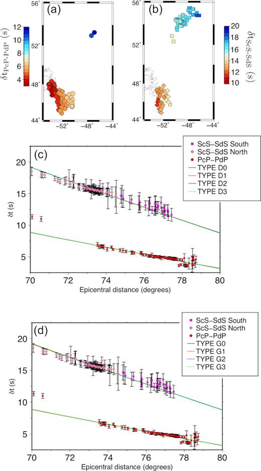
Differential traveltime measurements plotted on maps for δtPcP − PdP (a) and δtScS − SdS (b) and as a function of the epicentral distance (c, d). For the maps, the measurements are represented at the reflection point of the core-reflected wave. For the graphs (c, d), the uncertainties correspond to the standard deviation of the Gaussian distribution obtained with the bootstrap analysis (see Fig. 3). In (c) and (d) the traveltime delays predicted by the obtained best-fitting models D0–D3 and G0–G3 are superimposed (see text and Fig. 6 for details).
Summary of the number of processed data and detected waves.
| P data | S data | |
|---|---|---|
| Downloaded data set | 711 | 711 |
| After SNR selection | 521 | 529 |
| Number of subarrays | 428 | 438 |
| Detected waves | ||
| P/S only | 90 | |
| P & PcP / S & ScS | 181 | 224 |
| P, PcP and PdP / S, ScS and SDS | 110 | 135 |
| Bad quality | 47 | 79 |
| Measured traveltimes | ||
| PcP-PdP / ScS-SdS | 79 | 107 |
3.1 Bayesian inversion
The average trend of the delay times with the epicentral distance (Figs 4c and d) indicates that, in the regions where we detect a D″ reflection, they can be explained by a 1-D model including a flat D″ layer. We thus invert the traveltime measurements for D″ interface properties. To do so we adopt a Bayesian approach (Tarantola & Valette 1982b), meaning that we will explore the model space. This model space is infinite so in order to render the inversion feasible, we separate the inversion into two steps. First, we find the models that best fit the traveltime delays, considering various model families. Then, we will use these best-fitting models to find the one that best reproduces the amplitudes on the vespagrams of the data (see workflow Fig. 5).
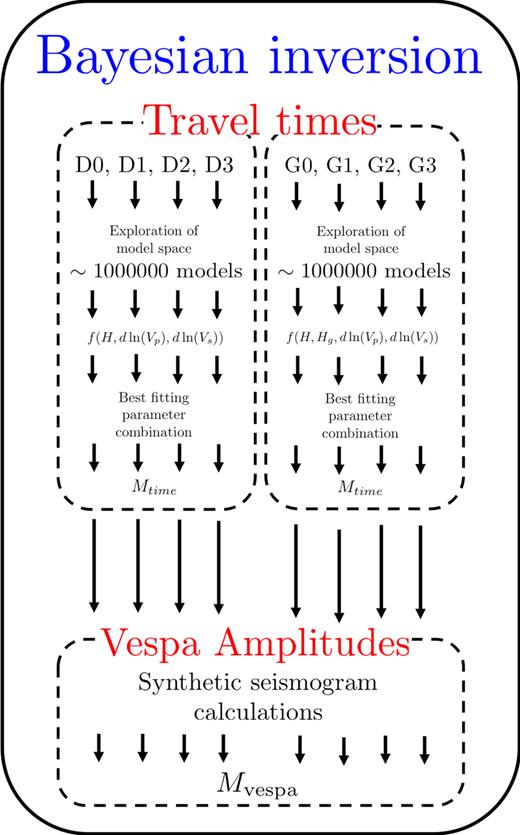
Workflow diagram of the Bayesian inversion. See text for misfit definitions and Fig. 6 for examples of models D0–D3 and G0–G3.
We define two distinct categories of models, category “D” and category “G”. Category “D” refers to models that are discontinuous across the D″ interface (”D” stands for ”discontinuous”). Within this category we then define four families (D0, D1, D2, D3) that differ from the slope of the velocity gradient inside D″ (Fig. 6a). These different gradients represent various heat fluxes at the CMB. Geodynamic modelling has shown that in regions where slabs are present, there is a decrease in temperature a few hundreds of kilometre above the CMB, followed by a sharp increase in temperature close to the CMB (e.g. Thomas et al. 2004b; Bower et al. 2013). Because there are large uncertainties on how to convert the temperature anomalies into velocity anomalies, we test several velocity profiles with velocity variations reproducing these temperature variations, where case D0 stands for an average mantle model including a D″ layer, such as in model pwdk (Weber & Davis 1990). These models are characterized by three free parameters that will be explored, the D″ thickness H and P- and S-wave velocity jumps across the D″ interface, dln (Vp) and dln (Vs), respectively. Category 'G' refers to models where we allow for a gradient at the top of D″ ('G' stands for 'gradient'). Again, we consider four families of models in that category (G0, G1, G2, G3) which differ from the slope of the velocity gradient inside D″ (Fig. 6b). These models are characterized by four free parameters that will be explored, the D″ thickness H, the gradient thickness Hg and P- and S-wave velocity jumps across the D″ interface, dln (Vp) and dln (Vs), respectively.
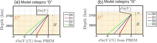
Examples of tested D″ velocity models with respect to PREM. In category “D” (a), the models are characterized by a D″ of thickness H and by S- and P-wave velocity jumps across the D″ interface dln (Vs) and dln (Vp). In category “G” (b), we investigate the sharpness of the D″ discontinuity by allowing for a gradient of thickness Hg at the top of D″. See Table 2 for the explored ranges of values for every parameter.
Summary of the explored parameters and parameter ranges for each family of models.
| Category | Model family | Parameter | Range | Step |
|---|---|---|---|---|
| D | D0, D1, D2, D3 | H | from 280 to 340 km | 1 km |
| dln (Vp) | from −3 to 4 per cent | 0.1 per cent | ||
| dln (Vs) | from −3 to 4 per cent | 0.1 per cent | ||
| G | G0, G1, G2, G3 | H | from 280 to 310 km | 2 km |
| Hg | from 1 to 60 km | 2 km | ||
| dln (Vp) | from −3 to 4 per cent | 0.1 per cent | ||
| dln (Vs) | from −3 to 4 per cent | 0.1 per cent |
An example of this procedure is shown in Fig. 7 in the case of model family D0. Fig. 7 represents the 1-D and 2-D (coloured faces) marginal probability densities. By fitting the 1-D marginal probability densities with Gaussian functions (red dashed curves in Fig. 7), we find that the best-fitting model for the model family D0 has a D″ layer of 305 (±7.7) km thick, with dln (Vp) = 0.8( ± 0.06) per cent and dln (Vs) = 1.00( ± 0.14) per cent. These values also enable us to compute the bulk sound velocity perturbation dln (Vϕ) = 0.68( ± 0.01) per cent. Tables 3 and 4 summarise the obtained best-fitting model parameters, as well as the associated misfit values Mtime for this first category of discontinuous models (D0–D3). We always find a D″ layer of around 300 km thick as well as positive P- and S-wave velocity jumps across the D″ interface. Interestingly, even though one would expect a strong trade-off between seismic velocities inside D″ and D″ thickness, we obtain a well resolved maximum because we benefit from a good distance coverage (see Fig. 2). This procedure would fail when inverting a single measurement.
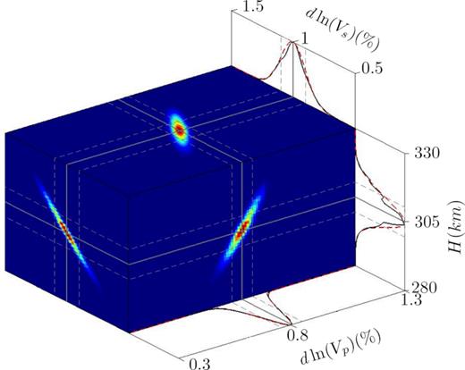
Representation of the a posteriori probability density, f(dln (Vs), dln (Vp), H) in the case of Hg = 0 for model D0. Every face is a 2-D marginal probability density showing the probability of two parameters to be the best-fitting model whatever is the third parameter. The three solid black curves represent the 1-D marginal probability densities (see eq. 4) of one parameter to be the best-fitting model whatever are the two others and the superimposed red dashed curves are the best-fitting Gaussian functions that yield the final values of every parameter with their uncertainties.
Summary of the velocity increases [dln (Vs), dln (Vp), dln (Vϕ)] across D″ as well as the corresponding traveltime delay misfit (Mtime) and vespagram misfit (Mvespa) for the best-fitting models (see text and Fig. 6 for details).
| Model family | dln (Vs) ( per cent) | dln (Vp) ( per cent) | dln (Vϕ) ( per cent) | Traveltime delay misfit (Mtime) | Vespagram misfit (Mvespa) |
|---|---|---|---|---|---|
| D0 | 1.00 ± 0.14 | 0.80 ± 0.06 | 0.68 ± 0.01 | 1.19 | 1.76 |
| D1 | 2.19± 0.11 | 2.37 ± 0.04 | 2.08 ± 0.01 | 1.19 | 1.72 |
| D2 | 2.90 ±0.11 | 3.10 ± 0.03 | 2.77 ± 0.02 | 1.19 | 1.70 |
| D3 | 3.63 ± 0.09 | 3.85 ± 0.02 | 3.50 ± 0.02 | 1.19 | 1.70 |
| G0 | 0.99 ± 0.12 | 0.78 ± 0.05 | 0.65 ± 0.01 | 1.19 | 1.77 |
| G1 | 2.25± 0.10 | 2.05 ± 0.03 | 1.93 ± 0.015 | 1.19 | 1.72 |
| G2 | 2.92 ± 0.10 | 2.71 ± 0.03 | 2.59 ± 0.015 | 1.19 | 1.70 |
| G3 | 3.59 ± 0.08 | 3.37 ± 0.02 | 3.24 ± 0.02 | 1.19 | 1.70 |
| C1 | 1.18 | 1.01 | 0.92 | 1.19 | 1.74 |
| C3 | 2.19 | 2.32 | 2.11 | 1.20 | 1.68 |
Summary of the D″ thicknesses H, gradient thicknesses Hg and corresponding D″ depths for the best-fitting models (see text and Fig. 6 for details).
| Model family | H (km) | Hg (km) | D″ depth (km) |
|---|---|---|---|
| D0 | 305 ± 7.7 | 2586 ± 7.7 | |
| D1 | 307 ± 7.8 | 2584 ± 7.8 | |
| D2 | 309 ± 8.7 | 2582 ± 8.7 | |
| D3 | 312 ± 8.5 | 2579 ± 8.5 | |
| G0 | 291 ± 6.3 | 25.3 ± 3.0 | 2587 ± 9.3 |
| G1 | 291 ± 8.4 | 30.0 ± 3.8 | 2585 ± 12.2 |
| G2 | 294 ± 9.2 | 31.4 ± 4.8 | 2581 ± 14.0 |
| G3 | 296 ± 9.3 | 30.6 ± 5.4 | 2580 ± 14.7 |
| C1 | 100 | 200 | 2591 |
| C3 | 170 | 130 | 2591 |
In the case of model families G0–G3, the a posteriori probability functions are less well resolved for parameters H and Hg because of the trade-off between them. However, we are still able to find best-fitting models, that fit the data equally well as models D0–D3. The best parameter values and misfit Mtime values are given in Tables 3 and 4. In this family of models, we always find a D″ layer of thickness around 290 km with a 20 to 30-km-thick gradient layer at the top of the layer. The P- and S-wave velocity jumps are also always both positive and similar in values.
We verify a posteriori that all these models fit the data on Figs 4(c) and (d). The use of traveltimes alone does not enable us to choose between all these models because they fit the delay times equally well (delay time misfit values in Table 3). However, the best-fitting requires a comparison of the observed amplitudes to synthetic ones obtained for the best-fitting model of every family (D0–D3, G0–G3). To do so, we compute synthetic seismograms using the reflectivity method (Fuchs & Müller 1971; Müller 1985) with the PREM model (Dziewonski & Anderson 1981) as input, in which we include a D″ layer characterized by the best model parameter combinations given Tables 3 and 4. The reflectivity calculations also include an Earth’s flattening approximation. We assume that the effect of 3-D heterogeneities is small because we are using differential traveltimes that are mostly sensitive to the D″ region where the tomographic models are very smooth over the studied region (see e.g. Fig. 1c).
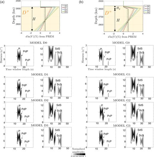
(a) Best-fitting models D0–D3 for Vp (dashed lines) and Vs (solid line) models with corresponding P and S vespagrams of synthetic traces. (b) Best-fitting models G0–G3 for Vp (dashed lines) and Vs (solid lines) models with corresponding P and S vespagrams of synthetic traces. The vespagrams have been computed for the same group of stations as those for the vespagrams of data shown Figs 2(b) and (d).
4 DISCUSSION
The seismic reflector at the top of D″ is generally associated with a phase transition from magnesium silicate bridgmanite (Br) to post-perovksite (pPv) (e.g. Sidorin et al. 1999; Murakami et al. 2004; Oganov & Ono 2004; Hernlund et al. 2005; Lay 2007b; Sun et al. 2008; Cobden et al. 2015). Several theoretical and experimental investigations have focused on determining the elastic properties of MgSiO3 Br and pPv as well as studies that estimate the effects of Al, Fe and H incorporation to these phases (see e.g. Caracas & Cohen 2005; Wookey et al. 2005; Mao et al. 2006; Stackhouse et al. 2006a, b; Tsuchiya & Tsuchiya 2006; Wentzcovitch et al. 2006; Grocholski et al. 2012; Townsend et al. 2015; Shukla et al. 2016; Zhang et al. 2016). Theoretical studies report that the phase transition of a pure MgSiO3 Br to pPv produces a positive jump in Vs, a small positive or negative jump in Vp and a negative jump in Vϕ (Wookey et al. 2005; Stackhouse et al. 2006b; Tsuchiya & Tsuchiya 2006; Wentzcovitch et al. 2006), which collectively do not match the observations in our study. Moreover, it has been shown that the presence of iron or aluminium increases the depth range that Br-pPv coexist (Akber-Knutson et al. 2005; Grocholski et al. 2012), such that, in the lower mantle, where bridgmanite is likely to contain some amounts of iron and aluminum, the phase transition is expected to be broadened (Akber-Knutson et al. 2005; Hirose et al. 2005; Caracas & Cohen 2007; Catalli et al. 2009; Grocholski et al. 2012). When combined with effects due to the possible presence of relatively cooler and chemically distinct slab debris (Grocholski et al. 2012; Bower et al. 2013), the sharpness and layer thickness of D″ will likely also be affected, which resemble features captured in the ”G” models.
Figs 9(a)–(d) show a summary of the areas and distances whereP or Swaves, reflected off D″, are detected. In Figs 9(a) and (b), we display the 'summary' map obtained for seismic P- and S-wave velocity perturbations extracted from six recent global tomographic models. The histograms in Figs 9(c) and (d) show that the different groups of detection do not correspond to particular distance ranges, they all overlap. Regions where D″ reflected waves are well correlated with regions where the velocity perturbations predicted by tomographic models are positive for both P- and S-wave velocity perturbations. Remnants from the ancient subduction of the Farallon plate have been inferred in the studied area (e.g. Bunge & Grand 2000; Conrad et al. 2004). Based on this inferrence, we tested additional models where we consider only two variations of heat fluxes at the bottom of D″, that are thus denoted C1 and C3 (referring to the denomination we used for model categories 'D' and 'G'). They are shown in Fig. 10 and their characteristics are given Tables 3 and 4. They are characterized by a sharp D″ interface, with jumps in P- and S-wave velocities that then extend farther down before decreasing towards the CMB (e.g. Sidorin et al. 1998; Thomas et al. 2004b; Sun et al. 2008). In these velocity models, the depth range with higher velocities mimics the presence of a thermochemical/phase boundary that could represent the presence of a thermal slab interacting with a phase transition. Although we did not perform a Bayesian inversion for models C1 and C3, we compute the misfit values (Table 3). We find that model C3 better reproduces both traveltimes and wave amplitudes than any other models.
![(a, b) Maps summarizing the different detected waves for P (a) and S (b) data. They are represented at the reflection point of the core-reflected wave on top of a summary map (e.g. Lekic et al. 2012) obtained considering six tomographic models [S40RTS (Ritsema et al. 2011), SEMUCB-WM1 (French & Romanowicz 2014b), S362WMANI+M (Moulik & Ekström 2014), SGLOBE (Chang et al. 2015), SP12RTS (Koelemeijer et al. 2016), SEISGLOBE2 (Durand et al. 2017)] at 300 km above the CMB. The colorbar on the right of panels (a) and (b) indicates the number of models out of the six considered that report a positive velocity anomaly in the area. The cases where PcP is not detected are shown as filled black circles. (c, d) Histograms of the different detected waves, where the colors are defined to the right of panels (c) and (d).](https://oup.silverchair-cdn.com/oup/backfile/Content_public/Journal/gji/216/2/10.1093_gji_ggy476/1/m_ggy476fig9.jpeg?Expires=1750363164&Signature=w5jFtOPXfCkivBOdtVJK8kbl8M6MqnLxIKOJ6YWRv1vzVrHUZDmmWplKmRlMoJdd2y0ptNHkLaBD0QrSqcnJvZw~WI9t~19VzXS0yrRVEiMJiP~zzBhtQmIEZZ0cWluxte9fcZvtSL5gxuNFpAQPL5U7D~pyuLAkiLCT6-KmDuahSPTMYSeq~xPrBf1gvvm1rQz5Pxc2100r9w4qkGSoRzMJ8bPv7NdPtXzsam~F~jdXYkRgHdGvxRY0IFtUvDd9ozjzoaO906HedkPjLFXb5DejjoA~oevdufGN6PNbdeKoj187mKlE3zaYAH-C045FLv~w5NxYaujxsxRiOWSq2g__&Key-Pair-Id=APKAIE5G5CRDK6RD3PGA)
(a, b) Maps summarizing the different detected waves for P (a) and S (b) data. They are represented at the reflection point of the core-reflected wave on top of a summary map (e.g. Lekic et al. 2012) obtained considering six tomographic models [S40RTS (Ritsema et al. 2011), SEMUCB-WM1 (French & Romanowicz 2014b), S362WMANI+M (Moulik & Ekström 2014), SGLOBE (Chang et al. 2015), SP12RTS (Koelemeijer et al. 2016), SEISGLOBE2 (Durand et al. 2017)] at 300 km above the CMB. The colorbar on the right of panels (a) and (b) indicates the number of models out of the six considered that report a positive velocity anomaly in the area. The cases where PcP is not detected are shown as filled black circles. (c, d) Histograms of the different detected waves, where the colors are defined to the right of panels (c) and (d).
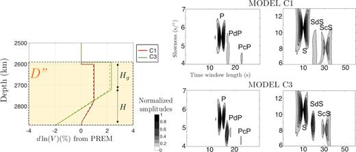
(a) Best-fitting models C1 and C3 for Vp (dashed lines) and Vs (solid line). (b) P vespagrams of synthetic traces. (c) S vespagrams of synthetic traces. The vespagrams have been computed for the same group of stations as those for the vespagrams of data shown Figs 2(b) and (d).
Considering all the explored models in our study, the ones that best explain our seismic observations are models C3, D2–D3, G2–G3. They are all characterized by positive and strong P- and S-wave velocity jumps across the D″ interface and by a reduction in wave speeds down to the CMB. Models D2–D3 and C3 have a sharp D″ interface, but for model C3 it extends down to about 100 km, while models G2–G3 are characterized with a gradient (reduced sharpness) at the top of the D″ layer. Based on the misfit values it is difficult to distinguish all these models. Model C3 appears slightly better, but since it has not been obtained after a proper Bayesian inversion we prefer not to draw further conclusions. Nevertheless, our study rules out a decrease in wavepseeds as well as velocity increases smaller than 2.7 per cent in both P- and S-wave velocities at the D″ interface, indicating that a pyrolitic Br to pPv transition is unlikely to explain these observations (e.g., Cobden et al. 2013). Models with no velocity reduction above the CMB are also ruled out.
It has been shown that the enhanced aluminium and iron concentrations in mid-oceanic ridge basalt (MORB) subjected to the pressure–temperature conditions of the lowermost mantle broadens the Br-pPv phase transition (Akber-Knutson et al. 2005; Hirose et al. 2005; Caracas & Cohen 2007; Ohta et al. 2008; Catalli et al. 2009; Grocholski et al. 2012) and is compatible with an increase in Vϕ at the transition (e.g. Cobden et al. 2013). If slab debris similar to that of MORB has accumulated in this region, then a broader seismic 'transition' (or gradient) and perhaps cooler temperatures (Ohta et al. 2008; Grocholski et al. 2012), such as our models G2–G3 and C3, may be expected due to these phenomena. However, the detailed chemistry of the assemblage cannot be identified because several factors remain uncertain: the pressures–temperatures of the pPv appearance and Br disappearance in slab debris, the partitioning of Fe/Mg between coexisting Br, pPv and other phases, and the effect of compositional variation on these variables.
We also observe some cases where the P wave reflected off the CMB, namely PcP, is not visible (Fig. 9a, black circles), but we do not find such cases for ScS (see Fig. 9b). This is expected from the reflection coefficients off the CMB that are close to 1 for S waves, but which vary for P waves. The area between the Northern SdS detections and the southern PdP and SdS detections does not seem to produce either PdP or SdS reflected waves. We first tested whether these lateral variations could be due to the source mechanism by computing the radiated P, PcP, S and ScS energies, but we found no correlation between the radiation pattern and the detection pattern. The absence of PcP and PdP or SdS could also be due to out-of-plane propagation, possibly generated by D″ or CMB topography (see e.g. Sun et al. 2008). However, we performed slowness/back-azimuth analysis (Rost & Thomas 2002; Schweitzer et al. 2002) and no systematic evidence of such an effect was found; most of our detected waves travelled on the great circle path and those event-receiver combinations without PcP, PdP or SdS did not show out-of-plane signals that could be attributed to core and D″ reflections. Seismic anisotropy or small impedance contrasts could also explain the lack of PcP, PdP and SdS waves. All these hypothesis could be tested using crossing raypaths sampling the same region, however, the limited number of earthquake-station combinations suitable to study the D″ structure in this area does not allow this verification. Alternatively, the absence of detected D″ reflected waves could also be explained by significantly higher temperatures such that a phase transition to pPv would be suppressed. Indeed, as suggested by geodynamical modeling (Bower et al. 2013; Sun et al. 2016), the presence of the slab could create an anomalously high heat flux in front of the slab which would deepen the Br-pPv phase transition and, if the temperature anomaly reaches several hundreds of Kelvin (Hirose et al. 2005), the Br-pPv phase transition may not occur. This latter situation would generate complex material flow, from horizontal flow in the slab region to upward flow in the warmer region, a hypothesis that could be tested in future studies investigating the presence of anisotropy.
One can also observe that even though all our models well fit the traveltime delay (Figs 4c and d), the fit is worse for distances smaller than 72° which corresponds to the North area of the studied region. The larger delay times in P would indicate a slower P velocity. However, these two data points are not sufficient to bring further constraints and this again requires further investigation.
To summarize, the areas where we detect D″ reflected waves can be explained by the presence of relatively cold ancient Farallon slab debris, that has been inferred for this region before (models D2–D3, G2–G3 or C3). The slab debris, in the form of MORB-rich material, would undergo a broad phase transition (reduced sharpness of D″) due to enhanced aluminium and other elements. This applies for the North and South areas. It is important to note that in the North area, the D″ reflector is only detected with S waves, and not with P waves. This could result from the presence of small scale scatterers affecting preferentially high frequency P waves (e.g. Rost et al. 2010; Frost et al. 2013; Ma et al. 2016; Frost et al. 2017). In the regions where the D″ reflector is not detected at all, neither with S nor with P waves, various explanations are possible: (1) small D″ topography that deviates the waves which are thus not observed, (2) seismic anisotropy or (3) an anomalously high heat flux in the front of the remnant slab. These interpretations and hypotheses are summarized in Table 5.
Summary of the various interpretations.
| Region | Observations | Preferred models | Interpretation |
|---|---|---|---|
| North area | SdS, no PdP | D2–D3, G2–G3, C3 | Presence of (cooler) MORB-like debris from ancient Farallon slab |
| Br to pPv phase transition in a Fe- and Al-enriched assemblage small scale scatterers | |||
| Central area | no SdS, no PdP | no D″ reflector | D″ topography, anisotropy |
| Presence of a nascent hot plume that inhibits the Br-pPv phase transition | |||
| South area | SdS, PdP | D2–D3, G2–G3, C3 | Presence of (cooler) MORB-like debris from ancient Farallon slab |
| Br to pPv phase transition in a Fe- and Al-enriched assemblage |
5 CONCLUDING REMARKS
In this study, we show that by combining both P and S observations we are able to propose the most likely characteristics of the D″ layer beneath the North Atlantic. To do so we performed a bootstrap analysis in order to measure traveltimes that were then inverted for P- and S-wave velocity perturbations and D″ thickness, applying a Bayesian inversion. We investigated the sharpness of the D″ discontinuity as well as the existence of a negative velocity gradient towards the CMB. Combined with further synthetic seismogram calculations, that were used to compare with the observed seismograms, we find that the best-fitting models have a D″ thickness of 300 km as well as strong and positive velocity jumps across the D″ discontinuity ranging from 2.7 to 3.8 per cent for both Vp and Vs. We also find that a velocity gradient across the D″ interface of ∼30-km thick or a 100 km thick fast region at the top of D″ equally well explains the data. These results suggest that the D″ layer beneath the North Atlantic region could be characterized by a broadened Br-pPv phase transition in subducted slab debris. Lateral variations in the detection of D″ in our region further point towards the presence of heterogeneities, in the form of temperature, composition, topography, anisotropy or a combination of these.
ACKNOWLEDGEMENTS
The authors thank M. Thorne, D. Frost, and one anonymous reviewer for their helpful comments as well as the Editor Martin Schimmel. Data were analysed with Obspy (Beyreuther et al. 2010), maps were drawn with GMT (Wessel & Smith 1991) and the tomographic section was obtained with SeisTomoPy (Durand et al. 2018). Data were downloaded with IRIS. S.D. was supported by the DFG project HAADES DU1634/1-1. J.M.J. was supported through the International Office of WWU, Münster, NSF-CSEDI-EAR-1600956, Caltech, and the W.M. Keck Institute for Space Studies.
