


SUMMARY
To study the characteristics of seismicity in Italy, we have made use of the ISIDE (Italian Seismic Instrumental and parametric Data-basE) catalogue since 2005 April 16, which was compiled by the Istituto Nazionale di Geofisica e Vulcanologia (INGV). This catalogue includes high quality records of the occurrence times, locations, magnitude and other information about the earthquakes that occurred in and near Italy. We made use of the original form and two extended versions of the space–time ETAS model, namely, the 2-D ETAS model, the hypocentral 3-D ETAS model and the finite-source (FS) ETAS model. Our results show that the rupture geometries of large earthquakes, including the L’Aquila (2009 April 6 Mw6.1/ML5.9 ), the Finale-Emilia (2012 May 20, Mw5.8/ML5.9), the Amatrice (2016 August 24 Mw6.0/ML6.0) and the Norcia (2016 October 30 Mw6.5/ML6.1) earthquakes, control the spatial locations of their direct aftershocks. These direct aftershocks are mainly distributed in some areas adjacent to, but seldom at, the parts with the biggest slips along the main shock rupture, implying that aftershocks compensate the rupture of the main shock. The background seismicity rate is not stationary in all these areas, but shows several phases tuned by the major events. Regarding the difference among the three versions of the ETAS model, we found: (i) hypocentral depth plays an important role in triggering; (ii) when classifying background and triggered seismicity, all three models give similar results, but when classifying the family trees in the catalogue, the geometry of an earthquake rupture should be considered. The FS ETAS model classifies most aftershock events as aftershocks of the main shock; (iii) adopting point sources together with isotropic spatial response causes underestimates of the effects triggered by the main shocks. Such biases can be corrected by incorporating the rupture geometries of major events into the model formulation. Compared to the original point-source model, more direct aftershocks from the main shock are estimated by using the FS ETAS model and (iv) The rupture geometry of a major earthquake can be inverted to some extent from small aftershocks following it by fitting to the finite-source ETAS model.
1 INTRODUCTION
Since August 2016, a sequence of ML5.5 earthquakes occurred in Italy, including the ML6.0 Amatrice earthquake on 2016 August 24, the ML5.9 Visso earthquake on 2016 October 26 and the ML6.1 Norcia earthquake on 2016 October 30. These earthquakes and their aftershocks caused considerable loss of human life and property damage (e.g. Chiaraluce et al.2017). For example, the Amatrice earthquake caused the death of 299 people and economic loss which is roughly estimated at up to 17 billion dollars, according to reports by newspapers, such as The Telegraph (https://www.telegraph.co.uk/news/2016/08/24/italy-earthquake-at-least-73-dead-including-many-children-as-apo/). In addition to the loss of human lives, widespread destruction of cultural heritage sites was also reported.
To provide more reliable information about the occurrence of an ongoing seismic sequence, a complete understanding of the seismicity pattern is indispensable. The aim of this study was to understand the clustering characteristics of seismicity in the time period 2005–2016, during which the ISIDE (Italian Seismic Instrumental and parametric Data-basE) catalogue was compiled by the Istituto Nazionale di Geofisca e Vulcanologia (INGV), Italy. The basic tool for this is the Epidemic-Type Aftershock Sequence (ETAS) model, which has been widely and successfully used to quantify the clustering patterns of seismicity. Its early version only focused on earthquake occurrence time (Ogata 1988, 1989, 1992) and was generalized by Ogata (1998) to the space–time ETAS model by incorporating both the earthquake locations and occurrence times. This version and its variations became the standard model in data analysis (see, e.g. Console & Murru 2001; Helmstetter & Sornette 2002, 2003; Console et al.2003, 2006, 2007; Ogata et al.2003; Ogata 2004; Zhuang et al.2004; Hainzl & Ogata 2005; Zhuang et al.2005; Helmstetter et al.2006; Zhuang et al.2008; Marzocchi & Lombardi 2009; Lombardi et al.2010; Werner et al.2011; Zhuang 2011). Guo et al. (2015a, 2018) extended the ETAS model to a hypocentral 3-D version by incorporating the depth of earthquake hypocentres. Moreover, instead of regarding each earthquake in the catalogue as a point in space and time, Guo et al. (2015b, 2017) extended this model again by incorporating the fault geometry of large earthquakes into the model formulations, namely, the finite-source ETAS model. This inclusion is important because most of the aftershocks occur along the rupture fault of the main shock rather than being concentrated around the epicentre of the main shock. They also found correlations between aftershock productivity and the pattern of the coseismic slip, indicating that aftershocks within rupture faults are adjustments to coseismic stress changes due to slip heterogeneity.
In this study, we applied three versions of the ETAS model: the (2-D)-space–time ETAS model, the (3-D)-hypocentral ETAS model and the finite-source (FS) ETAS model to Italian seismicity in order to understand the seismicity patterns and clustering characteristics. This study also provided us the opportunity to study the advantages and limitations of each model. In the following two sections, we will firstly make a brief introduction to the data and then explain these ETAS models and related concepts and methods. In the sections on data analysis, we compare the results from fitting the models to the ISIDE catalogue to extract the clustering characteristics of seismicity in Italy and the surrounding region.
2 THE STUDY REGION AND DATA
The Italian region occupies a central position in the Mediterranean area, one of the most complex areas of the Earth from a geodynamic point of view (Fig. 1). This area is active due to the convergence between the African and Eurasian plates (e.g. Doglioni et al.1998). The Alpine chain, which is the result of the first stage of convergence, follows the southeastward immersion of the Alpine Tethys oceanic branches beneath the Adriatic continental Plate, a promontory of the African Plate (Handy et al.2010). From the Miocene to Pliocene the central Mediterranean was also dominated by a more recent tectonic phase with the opening of the Tyrrhenian basin and the creation of the Apennines chain that now forms a fold and thrust belt (Patacca & Scandone 1989). During the Quaternary, thrust tectonics gave way to extensional tectonics, with the development of a zone of normal faulting running along the crest of the mountain range. In the Central Apennines, the zone of extension is about 30 km wide and is characterized by a zone of observed extensional strain, as shown by GPS measurements (D’Agostino et al.2001, 2012; Serpelloni et al.2006; Pezzo et al.2015; Cheloni et al.2017). In contrast, the northern Apennines represents a frontal thrust system composed of a pile of NE-verging tectonic units that developed as a consequence of the collision between the European Plate and the Adria Plate (Boccaletti et al.2011). In the last 12 yr, these regions have been the most seismically active areas of Italy for some events greater ML5.5+.
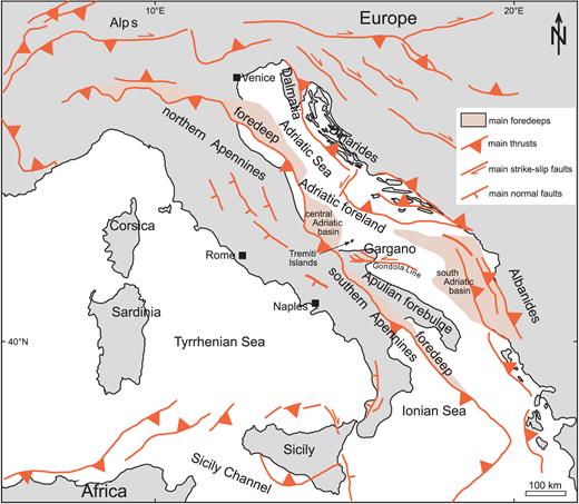
Tectonic structure in Italy and surrounding region (modified from Billi et al.2007).
In this study, we used the ISIDE catalogue compiled by INGV (http://cnt.rm.ingv.it/iside, ISIDE working group, 2016). We selected the data in the range of latitudes 35°–48°N, longitudes 6°–19°E and depths 0 to 70 km. The study interval in the catalogue extends from 2005 April 16 to 2017 January 27. The magnitude threshold was set to ML2.9, because the completeness magnitude in most parts of Italy, including aftershock sequences, is equal to ML2.9. In the selected space–time–magnitude–depth range, there were 4552 events. The local magnitude, ML, was used in the analysis process.
Fig. 2 shows the epicentral map of seismicity in Italy during the study period. Most of the seismicity was concentrated along the Apennines and the volcanic zones in Sicily (Etna and Eolie islands) and in the Sicily Channel. To the east, seismicity was dominated by the Adriatic foredeep.
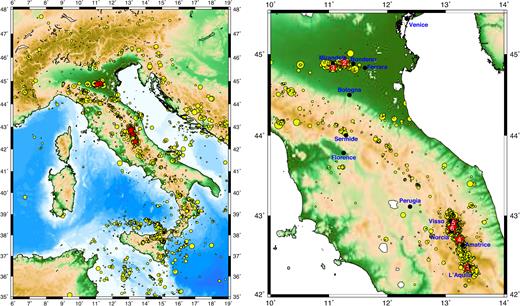
(Left-hand panel) Epicentre map of seismicity of ML ≥ 2.9 in the Italy region during the period from 2005 April 17 to 2017 January 27 and (right-hand panel). An enlarged map of the northern and central areas where the six major events were located. The red stars with numbers mark the six major earthquakes (ML ≥ 5.5) listed in Table 1.
Six events of M5.5+ occurred in the study space–time–magnitude–depth range. We will treat these events with special attention.
L’Aquila earthquake (LA). This MW6.1 earthquake occurred at 03:32 local time (01:32 UTC) on 2009 April 06 in the Abruzzi region in central Italy, causing the death of more than 300 people and destroying the city of L’Aquila and many surrounding villages. Its epicentre was located on one NW–SE trending normal fault that forms part of the 800-km-long segmented normal fault system that accommodates crustal extension in the Apennine mountain range (e.g. Anderson & Jackson 1987; Roberts et al.2002). Its hypocentral depth was 8.3 km, within the seismogenic layer in this area, of which the depth ranges from 2 to 10 km. Its 18 km rupture extended northwestward, with a dip angle of 45° and a rake angle of –102° (Chiarabba et al.2009; Cirella et al.2009). This earthquake was accompanied by a foreshock sequence and produced a sequence of many aftershocks.
Finale-Emilia (FE) and Mirandola (MR) earthquakes in the Emilia-Romagna region. These 2012 Northern Italy earthquakes were two of the major earthquakes that occurred in Northern Italy since the beginning of our data set. They caused 27 deaths and widespread damage. In Italy they are better known as the 2012 Emilia earthquakes.
The first earthquake, with a magnitude of Mw5.8/ML5.9, occurred about 36 km north of the city of Bologna in the Emilia-Romagna region, on 2012 May 20 at 04:03 local time (02:03 UTC). The hypocentre was located between Finale Emilia, Bondeno and Sermide at a depth of 9.5 km. Two aftershocks of magnitude ML5.0 occurred, one approximately four minutes and the other 1 hr after the main event. Seven people were killed.
A moment magnitude 5.6 earthquake struck the same area 9 d later, on 2012 May 29 at a depth of 8.1 km. The epicentre was near the town of Mirandola, about 12 km west–southwest of the main shock (Scognamiglio et al.2012). This second main shock started a new aftershock sequence in this area and increased structural damage and collapse, causing 19 more casualties and increasing to 15 000 the number of evacuees, as the buildings already weakened by the 2012 May 20 earthquake.
Amatrice earthquake (AM). The Amatrice earthquake with moment magnitude of 6.0, hit Central Italy on 2016 August 24 at 03:36:32 local time (01:36 UTC) starting the ongoing central Italy seismic sequence. No conventional foreshocks occurred in the months beforehand. Its epicentre was close to the towns of Accumoli and Amatrice, with its hypocentre at a depth of 8.1 km, approximately 75 km southeast of Perugia and 45 km north of L’Aquila, in an area near the borders of the Umbria, Lazio, Abruzzi and Marche regions. in the 2016 August 24 earthquake, 299 people were killed, according to the Civil Protection Department of Italy. This initial earthquake was followed by the largest aftershock (ML5.4) almost one hour after the main shock. It was located 12 km NW from the main shock and close to the town of Norcia. In the first month, about 2500 aftershocks of ML ≥ 2.0 were observed, among which 15 earthquakes were greater than ML4.0 (Gruppo di Lavoro INGV sul terremoto di Amatrice 2016). The main shock and a number of aftershocks were felt across the whole of central Italy.
Visso earthquake (VS). Two months later, on 2016 October 26 at 21:18 local time (19:18 UTC), another main shock with a moment magnitude of 6.1 occurred 25 km to the north of the Amatrice earthquake, near the town of Visso. It showed clear overlap with the southern termination of the 1997 Colfiorito seismic sequence faults. This earthquake activated another normal fault segment approximately located on the along-strike continuation of the first structure. This earthquake was initially considered an aftershock of the Amatrice earthquake.
Norcia earthquake (NC). Four days after the Visso earthquake, on 2016 October 30 at 08:40 local time (06:40 UTC), the largest shock of the ongoing central Italy sequence, hit with moment magnitude of 6.5 in the area between the two previous events, destroying Norcia and surrounding towns. This event nucleated at a depth of 9.2 km, generated new and larger ruptures at the surface, sometimes exceeding those activated by the Amatrice shock. This indicates that the event occurred on the same fault system presently reaching about 60 km in length, and showed clear overlap with the southern termination of the 1997 Colfiorito seismic sequence faults. The Norcia earthquake is the largest event to have occurred in Italy since the Mw6.9 Irpinia earthquake that took place on 1980 November 23 in the southern part of Italy.
3 CONCEPTS AND METHODS
3.1 Model formulations
In this study, we considered three versions of the epidemic-type aftershock sequence (ETAS) model, namely 2-D, 3-D hypocentral, and finite-source (FS) ETAS models. For general discussions, we have used common notations such as λ, and used subscripts for each particular version, such as λ2D, λ3D and λFS. The common assumptions of these three versions of ETAS models are (Zhuang et al.2002, 2004, 2005; Zhuang & Ogata 2006; Zhuang et al.2008): (1) The background seismicity is a stationary Poisson process; (2) every event, no matter whether it is a background event or it is triggered by a previous event, triggers its own offspring independently; (3) the expected number of direct offspring is an increasing function of the magnitude of the mother event and (4) the time lags between triggered events and the mother event follow the Omori–Utsu formula (Utsu 1970).
3.2 Maximum likelihood estimate
In the above finite-source ETAS model, both μ(x, y) and τi(u, v) are unknown functions. To estimate them and the model parameters simultaneously, an iterative algorithm that involves the stochastic reconstruction method (Zhuang et al.2002, 2004; Zhuang 2006, 2011) was used (Guo et al.2017). We refer readers to the Appendix for details.
3.3 Stochastic declustering
The stochastic declustering method classifies earthquake events into two classes: background events and triggered events (Zhuang et al.2002, 2004). The triggered events are grouped into different subprocesses, each of them being triggered by a particular mother event. Such a classification can be detailed onto each patch of the rupture plan for finite-source events. In the following paragraphs, we make a brief review of this method and then extend it to the case of the finite-source ETAS model.
![An illustration of stochastic declustering. The length of each segment represents the value of corresponding probability. Event i has a finite source with ni patches. U is a random number uniformly distributed in [0, 1]. In the figure, U falls in segment ρkj, indicating that event k is appointed as the mother event of j.](https://oup.silverchair-cdn.com/oup/backfile/Content_public/Journal/gji/216/1/10.1093_gji_ggy428/1/m_ggy428fig3.jpeg?Expires=1750229451&Signature=qXDGmjTCZ4QPyYmAuCJTplFTyTnsGwv32lZRElOo4Os8hSOm4GnvGOrIIGLNO79rbMy4pNII7XsYLGPBfuCFV-gcIRd7AQeWDlT42DWAgCIhlKpEoHrHkp6LW4EQh5QECfAw20Duk5oTKaiXsoo-meIMczlsDov9AD6TA4Qhp6lbrXwHqyQQHOl7HmatXyBAUakP5zcLvGqQPC4ndiLVKbnrahdnEG4mmvrM0TZXftyxVOP~5eUQuJ4jvPL~53K-2L-uvAdd~fBT8yL9blEkG4G1JBecXbmXFKJbf94WAdoZvdJ6H-W3HRlHblCRlYPpakS4BdknbnTa4wGhUecHRQ__&Key-Pair-Id=APKAIE5G5CRDK6RD3PGA)
An illustration of stochastic declustering. The length of each segment represents the value of corresponding probability. Event i has a finite source with ni patches. U is a random number uniformly distributed in [0, 1]. In the figure, U falls in segment ρkj, indicating that event k is appointed as the mother event of j.
One might ask why the most likely event is not always chosen to be the parent of the jth event for each j, or why this event is not always set as a background event if the background probability j is the highest among φj and ρij, i = 1, 2, ⋅⋅⋅, j − 1. This is because this alternative method can easily produce a biased influence on the declustering results. The reason can be explained with a simple example. Suppose that there are 100 events, where the background probabilities for each event are all 0.6. If we use the most likely probability to classify events, all the events are classified as background events, while the stochastic declustering method still classifies 40 per cent of the events as triggered events on average.
4 DATA ANALYSIS
4.1 Computation settings
Before carrying out the calculation for fitting the three models to the ISIDE catalogue, the following data pre-processing and computational parameters are set up.
Adding random noises to locations and depths. Our ETAS model requires that the observed process must be simple, that is there are no overlaps of events in time and location. Even though there are no simultaneous events in the ISIDE catalogue, some events overlap in epicentral location or depth because their epicentral locations are rounded off to the second digits in degrees and their depths rounded off to a digit in kilometres. For each event, we add a round error as a random number uniformly distributed within [–0.005, 0.005] degree and a rounding error as a random number uniformly distributed within [–0.5, 0.5] km.
Data buffer. In the calculation for fitting the ETAS model to the earthquake data, to avoid the biases caused by missing links between the triggering pair formed by an event outside and another event inside the target space–time region (Wang et al.2010; Harte 2013), a spatiotemporal buffer (complementary data set) is often used. Because there were no earthquakes larger than 5.5 within 2 yr before the starting time of this catalogue, and because no big clusters occurred in the first 3 yr, the time buffer was not used. For the spatial buffer, we fitted only the data in the polygon with vertices (12.8°E, 38.5°N), (14.7°E, 36.9°N), (16.0°E, 36.9°N), (17.6°E, 39.1°N), (16.3°E, 42.4°N), (11.3°E, 46.3°N), (8.4°E, 45.4°N), (14.5°E, 39.1°N) and (12.8°E, 38.5°N). The area within the data selection range (6°–19°E, 35°–48°N) but outside this polygon, is regarded as the buffer region. There is no depth buffer because the depth of 40 km is a clear boundary between clustered shallow events and isolated deep events. There was a total of 3746 events within the target polygon region. The fitting results were extrapolated to the entire range of data selection.
When smoothing the background rate for all three models, we used np = 4 and εmin = 0.02° (see eq. A2), that is the bandwidth for the jth event is the smaller one between the distance to its 4th closest event and 0.02°. For the 3-D model, the parameter η for controlling the beta kernel in smoothing the depth was ηz = 40 (see, eq. A5).
The patch size used in the calculation for the FS model is 0.02° × 0.02°. We selected a quite large region as the source zone for each major earthquake, expecting that it would cover the whole range of the source zone and that the estimate of the productivity from the patches outside the source zone would be near zero. For smoothing the productivity using eq. (A7) along patches, we used h = 0.01.
4.2 Basic fitting results
The fitting results are listed in Tables 2 and 3. Table 2 gives the estimated parameters from the model fitting and Table 3 shows the likelihoods for each model. The most significant result is in the likelihood. We note that for both the 2-D and FS models (with uniform depth and histogram depth) the log-likelihood increases by a factor equal to 3210.13 when the uniform distribution is replaced by the histogram depth. The 3-D model is the best model fit to the data, with an increment of 9165.37 in the log-likelihood from the FS ETAS model with empirical depth distribution. This implies that depth correlation plays an important role in seismicity triggering. Though the FS ETAS model is not the best fit, it has an increment in log-likelihood of 706.94 with respect to its 2-D counterpart. Why does the depth influence the fitting results so much? From Figs 4(a) and (b), we can see that the distribution of depths is not homogeneous and that members in an earthquake sequence have similar depths. For example, the depths of events in the 2009 L’Aquila, the 2012 Emilia and the 2016 Norcia sequences range from 6 to 14 km, 1 to 12 km and 2 to 17 km, respectively. The above facts explain why the 2-D or FS ETAS models with the histogram of depth as the depth distribution are better than the models with uniform depth distribution and why the 3-D ETAS models is better than the 2-D models. Fig. 4(a) also shows that the catalogue by INGV was not produced in a consistent way. At the beginning (in 2005) the default depth (the depth used when it cannot be determined properly) was 12 km, and this default depth was changed to 10 km from 2006 to 2014. There are also some events fixed at the default depths of 2 km and 5 km in areas where the seismicity was shallow during 2006 and 2014, but there were many fewer than those being put at the 10 km depth.
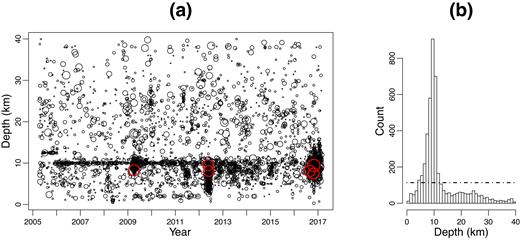
(a) Hypocentre depths versus occurrence times of shallow earthquakes (ML2.9+) occurring in Italy during the period from 2005 April 16 to 2017 January 27. (b) Histogram of depths. In (a), the different sizes of circles mark the magnitudes of earthquakes from 2.9 to 6.3 and the red circles represent the events of ML5.5 +. In (b), the horizontal dot-dashed line marks the average number of events over all the 2-km-depth intervals.
Major events (ML ≥ 5.5) in the study range.
| Index | Date and time (UTC) | Longitude | Latitutde | ML | Depth | Zone |
|---|---|---|---|---|---|---|
| (yyyy-mm-dd hh:mm:ss) | (°E) | (°N) | (km) | |||
| 1 | 2009-04-06 01:32:40.40 | 13.38 | 42.34 | 5.9 | 8.3 | L’Aquila (LA) |
| 2 | 2012-05-20 02:03:50.17 | 11.20 | 44.90 | 5.9 | 9.5 | Finale Emilia (FE) |
| 3 | 2012-05-29 07:00:02.88 | 11.07 | 44.84 | 5.8 | 8.1 | Mirandola (MR) |
| 4 | 2016-08-24 01:36:32.00 | 13.23 | 42.70 | 6.0 | 8.1 | Amatrice (AM) |
| 5 | 2016-10-26 19:18:05.85 | 13.13 | 42.91 | 5.9 | 7.5 | Visso (VS) |
| 6 | 2016-10-30 06:40:17.45 | 13.11 | 42.83 | 6.1 | 9.2 | Norcia (NC) |
Estimated parameters from fitting different ETAS models to the ISIDE catalog (2005 April 16 to 2017 January 27)
| Model | A | α | c (day) | p | D (10−4 deg2) | q | γ | Other |
|---|---|---|---|---|---|---|---|---|
| 2-D | .3214 | 1.542 | .01839 | 1.211 | 1.0752 | 2.455 | 1.1645 | |
| 3-D | .4856 | 1.043 | .01514 | 1.214 | 1.0440 | 2.171 | 1.0197 | η = 77.493 |
| FS | .1815 | 2.032 | .02609 | 1.218 | 1.2563 | 2.885 | 1.1027 | D′ = 1.0666 |
Comparison of likelihood among different models. PS and FS stand for Point Source and Fault Source, respectively, and Unif and Hist stand for the uniform and histogram depth distributions, respectively.
| Model | Log L |
|---|---|
| 2-D PS Unif | –5637.01 |
| 2-D FS Unif | –4930.07 |
| 2-D PS Hist | –2426.88 |
| 2-D FS Hist | –1719.94 |
| 3-D PS | 7445.43 |
| Model | Log L |
|---|---|
| 2-D PS Unif | –5637.01 |
| 2-D FS Unif | –4930.07 |
| 2-D PS Hist | –2426.88 |
| 2-D FS Hist | –1719.94 |
| 3-D PS | 7445.43 |
Table 2 also shows that the pair of parameters α and A are quite different in the three models. Parameter α is explained as the degree of difference in productivity among events of different magnitudes. A larger α means that more triggered events are generated by big events rather than by small events, while a lower α means that there is smaller difference in triggering offspring among events of different magnitudes. This indicates that the seismicity is more swarm-like. Extremly, when α = 0, all the events have the same productivity determined by parameter A. Parameter A, which represents the productivity from an event of the threshold magnitude, mc, has a negative correlation with parameter α in the estimation. As found by Hainzl et al. (2008), adopting an isotropic response function spatial in the ETAS model may cause low bias in the estimates of α value. Their calculated results confirmed this conclusion as did the results in Ogata (1998), Ogata & Zhuang (2006) and Guo et al. (2015b). As trade-off of parameter α, A is overestimated when α is underestimated. An increasing A value corresponds to a decreasing α value, and vice versa. This negative correlation was also noted by Harte (2015) when comparing the ETAS parameters that were used in simulating synthetic catalogues and their re-estimation. There were some minor differences in the model he used, from the 2-D model used here.
4.3 Classification of background events and family trees
By using the stochastic declustering method, we classified the catalogue into two subcatalogues, one of background events and the other of triggered events. The average numbers of background events classified for each ETAS model are in the second column of Table 4. They were estimated by averaging over many realizations or directly by summing over the background probabilities. The three models do not appear to be significantly different in classifying the background catalogue, with differences less than 2 per cent.
Estimated numbers of background events and model criticality.
| Model | Average # background events | Criticality |
|---|---|---|
| 2-D | 1716.7 | 0.793 |
| 3-D | 1729.6 | 0.808 |
| FS | 1748.5 | 0.788 |
| Model | Average # background events | Criticality |
|---|---|---|
| 2-D | 1716.7 | 0.793 |
| 3-D | 1729.6 | 0.808 |
| FS | 1748.5 | 0.788 |
Are these major events from the background or triggered? Fig. 5 plots the background probabilities versus occurrence times for each event. The three models give almost the same results. Among these six major events, five of them were triggered. This indicates that foreshock phenomena are significant in the Italy region. Any intermediate event should be taken into serious consideration whether it is a foreshock or not. Here we reference Marzocchi & Zhuang (2011) for detailed explanations of the foreshock probabilities in the Italian and Southern California regions based on the ETAS model.
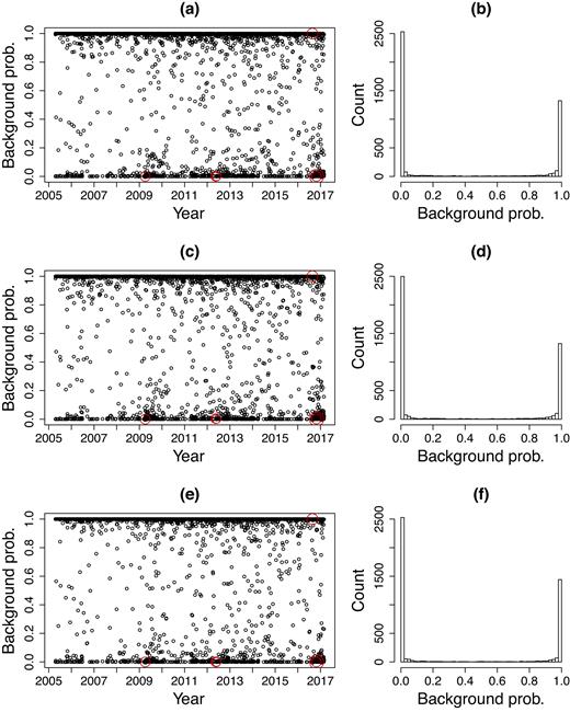
Background probabilities versus occurrence times of shallow earthquakes (ML2.9+) occurring in Italy during the period from 2005 April 16 to 2017 January 27 for (a) 2-D ETAS, (c) 3-D ETAS and (e) FS ETAS models and histograms of background probabilities for (b) 2-D ETAS, (d) 3-D ETAS and (f) FS ETAS models. In the left panels, the red circles represent the events of ML5.5 +.
The next step was to investigate the details of each family tree. Here we used the six major events as examples. Fig. 6 shows plots of the estimated numbers of direct offspring and all the descendants produced by the six major events (see Table 1) by using the three ETAS models. In all the cases involving the six major earthquakes, the FS ETAS model gives the largest numbers of direct offspring and the largest total numbers of descendants in all generations. The 2-D ETAS model gives less and the 3-D ETAS model gives the least. Especially for the 2016 Visso and the 2016 Norcia earthquakes, the 3-D ETAS model, which has the largest likelihood in parameter estimation, obtains both the numbers of direct offspring and all the descendants as small as close to zero. To understand why this happens, we plotted the estimated numbers of direct offspring and all the descendants produced versus occurrence times of all the events in Fig. 7. It can be seen from Fig. 7(c) for the 3-D ETAS model that some events smaller than the major events in the Emilia and the Norcia sequences produced more direct offspring than the corresponding major events did. In the case of the 2-D ETAS model, such situations are ameliorated and no earthquakes produce more direct offspring than the corresponding major events (Fig. 7a). The FS ETAS model gives the most satisfying classification where more events in each major cluster are classified as direct offspring from the major event (Fig. 7e).
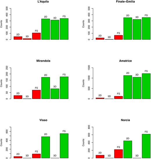
Estimated numbers of direct offspring (red) and all the descendants (green) produced by the six major events from using all three ETAS models.
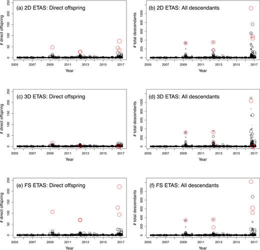
Estimated numbers of direct offspring and all the descendants produced versus occurrence times of all the events. The sizes of circles represent the event magnitudes from 2.9 to 6.3, and the six major events are marked in red.
Such misclassifications are caused by the isotropic spatial response kernel in the model formulation: (1) aftershocks are not distributed isotropically around the location of the cluster centre; (2) the main shocks are seldom located at the cluster centres; (3) regarding the source of a large earthquake as a pure point, but not a rupture with extension in space, exaggerates its distance to its direct offspring. Thus, it is not difficult to imagine that such anisotropy in the 3-D longitude–latitude–depth space can be reduced if the locations of the events are projected onto the 2-D longitude–latitude space of the earth surface. This explains why the 2-D ETAS model gives more reasonable classification results for the family trees in the catalogue than the 3-D one does. Looking back at Table 2, the classification results confirm the conclusion that a higher α implies that more events in the aftershock sequence are directly produced by the main shock but not by secondary or higher-order offspring.
4.4 Background rates
To study the background seismicity B(t), we divided the whole Italy region into 16 subregions, named R1 to R16 (Fig. 8). The division of these subregions is based on an overall consideration of the tectonic structures (Fig. 1) and the natural boundaries formed by the earthquake clusters and swarms. The cumulative background seismicity is plotted in Fig. 9. The results from the background seismicity rate can be summarized as follows:
First, the background rate is not always constant in each subregion, which is different from the assumption in the model formulation. The background rate is tuned by the six major events in 2009, 2012 and 2016.
Some areas show activation or quiescence before and after these major earthquakes. They are also some phases between major events, as in R2, R3, R4, R5, R8, R10. Such phases are either synchronic or occur after short time delays in different regions. The delays might be caused by fluid transport.
Basically, almost no difference appears in the estimates of background seismicity classified by the three models, especially the 2-D and 3-D ones. The finite-source ETAS model gives a relatively lower background rate in the aftershock zones (as in R4 for the 2012 Emilia sequence) and slightly higher background rates in the far field (as in R10 and R14-16).
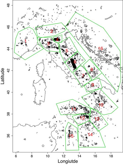
Subregions for studying background seismicity in Italy.
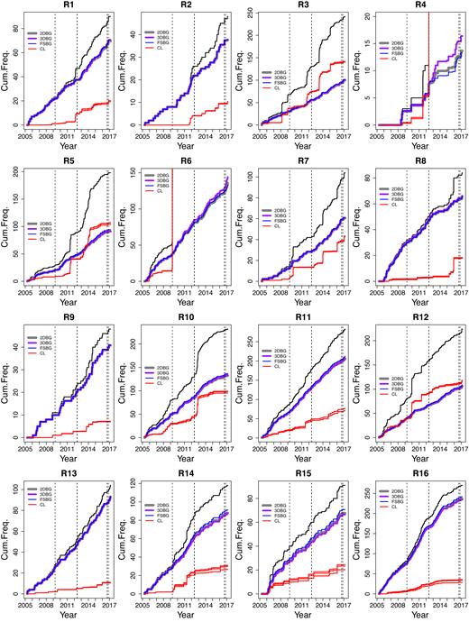
Cumulative background seismicity B(t) (see eq. 24) in each subregion, obtained by using the three ETAS models (2-D, 3-D, and FS, marked by 2DBG, 3DBG and FSBG, respectively) and compared to the cumulative seismicity (black curves) and cumulative clustering seismicity (CL, red curves). The vertical dashed lines mark the occurrence times of the six major events listed in Table 1.
4.5 Productivity heterogeneity on the rupture plane and their correlation to coseismic slips
Another useful product of the FS ETAS model is the direct offspring productivity due to each patch on the rupture plane of the major events. Using similarly as done by Guo et al. (2017), we plotted the contour image of the projection of the productivity of each patch onto the earth surface and compared these with the spatial distribution of coseismic slips caused by these major events, as shown in Fig. 10.
L’Aquila earthquake (2009 April 06, MW6.1, Fig. 10a). The kinematic source model was obtained by Scognamiglio et al. (2010, fig. 10B) from the joint inversion of strong motion and GPS data. It highlights two main rupture patches, updip from the hypocentre and southeast of the hypocentre along the strike propagation. The event has clear rupture directivity in both directions. The resulting model closely matches those obtained by Cirella et al. (2009, fig. 4) using similar data sets, and those by (Atzori et al. (2009), fig. 3a; Cheloni et al. (2010), fig. 4 a–b) using only geodetic data. The direct offspring of the L’Aquila main shock concentrate in two areas on the boundary of the main shock coseismic slipping area: one on the northwest of the epicentre and the other about 5 km southeast to the epicentre. Of much interest is that several moderate-magnitude aftershocks were clustered near the nucleation, consistent with the slip patterns (Cirella et al.2009). Despite the complexity of the rupture history of the L’Aquila main shock, we found that the results obtained by the FS ETAS model are consistent with the slip patches on the fault plane.
Finale-Emilia earthquake (2012 May 20, MW5.8, Fig. 10b). The coseismic slip model was obtained by Pezzo et al. (2013, fig. 6a) using geodetic data consisting of InSAR data and GPS site displacements. It shows whisker-shaped displacement patterns and has maximum slip to the south of the epicentre. The E–W oriented productivity of direct offspring mainly concentrates in three patches, from Mirandola to Bondeno, with the highest productivity from the southwest to the epicentre of this major event. Such productivity bounds the patches of relatively higher coseismic slip, confining the rupture boundary of the main shock. Directivity for the May 20 main shock is well detected, indicating that the rupture propagated unilaterally towards the SE (Cesca et al.2013, fig. 6). The other patch of aftershock locations (to the SE of Mirandola) could have triggered the occurrence of the 29 May event on the Mirandola fault. This suggests that the rupture of the Mirandola segment was induced by the productivity of direct offspring due to the May 20 event, which concentrated near Mirandola fault. In other words, that segment of the Mirandola fault was already prone to rupture, due to these aftershocks (Cesca et al.2013). Acceleration of the rupture occurred in the south-eastern portion of the fault plane, in agreement with the rupture directivity observed by Cesca et al. (2013). The imaged rupture process for Finale-Emilia agrees with the source mechanism and directivity array analysis proposed by Piccinini et al. (2012, figs 2-3), which clearly show the presence of two separate pulses on the relative source time functions computed using the empirical green function deconvolution for the May 20 earthquake.
Mirandola earthquake (2012 May 29, MW5.6, Fig. 10c). This coseismic slip model was obtained by Pezzo et al. (2013, fig. 4) in the same way as for the Finale-Emilia event. The highest productivity was mainly to the north of the epicentre, having the same direction as the area with the maximum coseismic Slip, but a bit further away. There is also a weaker slip patch to the west accompanied by a relatively lower productivity patch on its north.
Amatrice earthquake (2016 August 24, MW6.0, Fig. 10d). Here we use the slip model estimated by Tinti et al. (2016, fig. 4). In this slip model, the highest slip part is to the NEE of the epicentre and there is also a big area of relatively high slip about 6–7 km north of the epicentre. The productivity from the main shock mainly distributes around the northern high slip area in three patches. There are also two patches to the SSE direction of the epicentre with relatively lower productivity. In this case, earthquake clustering near Amatrice is consistent with the termination of causative fault of the major shock and might be associated with a portion of the Mount Gorzano fault. The sparse aftershock pattern to the northwest of the hypocentre, between Accumoli and Norcia, suggests a complex fault system with antithetic faults activated by aftershocks, and this is consistent with the location of the second slip patch near Norcia (Tinti et al.2016).
Visso earthquake (2016-10-26, MW6.1, Fig. 10e). The coseismic slip model obtained by Chiaraluce et al. (2017, figs 4 and 6) is compared with the productivity heterogeneity on the rupture planes obtained by the FS ETAS model. Their kinematic source models of the 2016 Central Italy earthquake sequence were inferred by inverting data recorded at tens of strong-motion stations located less than about 45 km of epicentral distance. The main parts of coseismic slips are distributed about 3 km north to the epicentre in the map. For this event, the maximum value of dislocation was about 80 cm. The direct offspring from the main shock are distributed further away from the main coseismic slip areas within a big patch with similar size to the north and two small patches to the northwest and west. The big patch indicates that the rupture propagation extended toward the north in the Colfiorito area, recently confirmed in terms of directivity by the coseismic slip distribution (Chiaraluce et al.2017).
Norcia earthquake (2016 October 30, MW6.5, Fig. 10f). The kinematic model adopted for the earthquake of Norcia (2016 October 30), as compared with the direct offspring, was explained in the previous point (Chiaraluce et al.2017). The main coseismic slip area is to the up dip from the hypocentre. The major parts of the direct aftershocks are located to the north and south of the area with the biggest coseismic slip. The patch of highest productivity that was situated close to the town of Norcia is probably due to activation of a secondary fault during the sequence (Cheloni et al.2017; Scognamiglio et al.2018). The patch to the North is related to the activity in the area of the maximum slip that occurred during the 2016 October 26 Visso main shock.
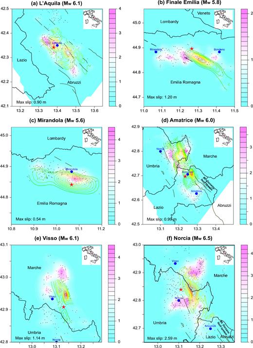
Comparison between the pattern of productivity of the direct offspring along the rupture areas (contour images) inferred by the FS ETAS model and coseismic slip (contour lines) for the (a) L’Aquila, (b) Finale-Emilia, (c) Mirandola, (d) Amatrice, (e) Visso and (f) Norcia events. The values of the coseismic slip from zero to the maximum for each event are shown by contour lines from green to red in rainbow colors. The red stars represent the epicentre of the corresponding major earthquake and the blue dots represent the locations of towns and cities in the area. The small black dots mark the locations of small events that occurred shortly after the corresponding major events. The traces of active faults are also plotted.
In summary, Figs 10(a) to (f) show that the direct offspring of the major shocks are mainly distributed around the area where the biggest coseismic slip occurs, but that these seldom overlap. This implies that aftershocks are the continuation of the main shock rupture. A fast estimation of the coseismic slip model for the source of a disastrous earthquake helps the estimation of hazard mitigation caused by large aftershocks, and vice versa. Rapid locating of the early aftershocks provides us useful constraints for inverting the coseismic slip model using strong ground motion and GPS displacement data.
5 CONCLUDING REMARKS
Using three versions of the space–time ETAS model, we studied the space–time characteristics of seismicity in and near Italy from 2005 to 2016. The conclusions from this study were divided into two aspects: the modelling and the seismicity. By comparison among these three models, we found that
The 2-D ETAS model, which is formulated with point sources for all the events isotropic spatial response to the triggering effect by previous events, underestimates the triggering productivity of large main shocks.
The 3-D ETAS model, which is also formulated with point sources but incorporates hypocentre depths, catches the depth information between triggering pairs in the catalogue and greatly improved the model fitting. This indicates that hypocentral depth plays an important role in triggering.
The Finite-source (FS) ETAS model is implemented by incorporating effects from the fault geometry of large earthquakes. The FS ETAS model corrects underestimates of α caused by isotropic spatial response in the point-source ETAS model, thereby enhancing the triggering of large events. It gives more reasonable classification of family trees in the catalogue: most triggered events are directly triggered by the main shock. This concept is consistent with the relatively high α values in Table 2. It also corrects estimates in the background rate, which should be higher in off-fault regions and lower in on-fault regions.
The finite-source (FS) ETAS model can be used to invert focal rupture geometry to some extent from location information about small events. We say ‘to some extent’ because it does not invert the coseismic or postseismic slips on the earthquake rupture plane, but does give the density of aftershock abundance along the rupture. The most productive areas along the rupture plane do not coincide with, but tend to be near the parts with the largest coseismic slips at a location. This implies that aftershocks are continuation of and compensation for ruptures of the main shock and that the spatial density of direct aftershock productivity along earthquake ruptures can be used as a constraint for inverting the slip model. This model was also useful for us to investigate patterns of direct aftershocks from mega events, which provides us with information regarding the evolution of aftershocks with coseismic stress changes or post seismic slips (e.g. Guo et al.2017).
When classifying background and triggered seismicity, all three models give similar results. However, when classifying the family trees in the catalogue, the geometry of the earthquake rupture should be considered. In the 3-D ETAS model, the effect of using the isotropic spatial response kernel becomes more serious than in the 2-D model. The FS ETAS model classifies most aftershocks as directly triggered by the main shock.
The uses of the isotropic kernel for triggered events, together with point sources for large events, cause underestimation of α and misspelled the family trees when decluttering the catalogue. From the τ-functions for the six major events obtained in this study and similar results obtained in Guo et al. (2015b, 2017), the complex fault ruptures are rather common and the spatial locations of aftershocks cannot be simply modelled as an elliptic response, which was also noticed by Harte (2014). With the introduction of finite-source modeling for the major events that have occurred in the area under analysis, we can correct the biased estimate of the value of α and provide a detailed estimate of how the aftershocks distribute along the rupture of the major earthquakes.
Considering that the 3-D model gvies the best data fit in likelihood among the three considered models, a more plausible model should be a 3-D model with fault geometry incorporated, that is a 3-D+FS ETAS model.
Regarding seismicity, we found that:
Seismicity in the Italy region is quite clustered. Using ML2.9 as the magnitude threshold, about 61 per cent of events can be explained by the triggered effect. Among the triggered events, more than a quarter are triggered directly by the five major earthquakes (Fig. 6 and Table 4). Among the six major earthquakes, five are marked as triggered events, indicating that foreshock phenomena are significant in the Italy region.
After dividing the whole study region into 16 subregions and separating the background events from the catalogue using the stochastic declustering method, we found that background seismicity in the entire Italian region is influenced by these major events. Those variations indicate different phases of seismicity caused by the major events.
In the rupture plane of the six strongest shocks in Italy from 2005 to 2016, direct aftershocks tend to occur near the parts with the largest slip on the rupture plane, but they seldom overlap, implying that aftershocks compensate the rupture of the main shock.
In summary, the results obtained applying the three different versions of the ETAS models (together with the stochastic declustering and the stochastic reconstruction techniques) using data from a high quality catalogue, combined with the Coulomb stress changes, and InSAR and GPS observations; allow us to better understand the geodynamic process in the Italian region. The results explain how seismicity can be used as a sensor to detect changes in the underground stress field, whether caused by major earthquakes or for other reasons. Also the spatial distribution of direct offspring productivity in the rupture area helps us to understand the dynamics of earthquake source processes. This distribution does not well overlap the coseismic slips, thus providing useful constraints for the inversion of the rupture process.
A commonly noticed problem in aftershock studies is the bias in the estimation of seismicity parameters caused by the short-term missing of aftershocks. It is well known that after a large event, many smaller events are missing from the catalogue because their waveforms cannot be distinguished from the coda of the major event. In this study, we do not consider these small missing aftershocks. Instead, we use a quite large magnitude threshold, ML2.9, above which most earthquakes are recorded. We notice that, although there are a few missing events of ML2.9 + after the 2012 Emilia and the 2016 Norcia events, the overall catalogue is acceptably complete. If a lower magnitude threshold is used, such missing of small events would cause some problems for model estimation. For example, in this case, the pure temporal ETAS model, which is immune to anisotropic distribution of aftershock locations, gives an under-estimated value of α (Zhuang et al.2017). Thus a question arises: Is the FS model immune from a lack of triggering from the missing events? The answer is ‘No’. From eqs (10) and (15), the productivity of the major events is still controlled by κ(m). Existence of missing short-term aftershocks causes under-estimation of the productivity of major events because the missing events, which are most likely to be direct offspring of the major events, are not counted as direct offspring of the major events in model fitting. The FS model only corrects the biases caused by isotropic modelling of the anisotropic aftershock response.
As mentioned by Box (1976, 1979): ‘All models are wrong, but some are useful’ and ‘Remember that all models are wrong; the practical question is how wrong do they have to be to not be useful.’ It can be seen from our analysis that none of the models is ideal. Even so, the 2D and 3-D ETAS models provide us with reliable declustering results for extracting background seismicity from the whole catalogue. However, when going into the details of the family trees of each cluster, the FS ETAS model is necessary. Considering that the 3-D model gives the best fit of the data by providing better forecasting information of event depths, we can conclude that a 3-D finite-source ETAS model is promising for analyzing earthquake catalogues at high resolution.
ACKNOWLEDGEMENTS
The authors thank Antonella Cirella, Rodolfo Console, Stefania Gentili, Rita Di Giovambattista, Taroni Matteo, Warner Marzocchi, Yosihiko Ogata and Elisa Tinti for helpful discussions as well as two anonymous reviewers for the their constructive comments.
REFERENCES
, eds
APPENDIX: ITERATIVE ALGORITHM FOR SIMULTANEOUSLY ESTIMATING MODEL PARAMETERS, BACKGROUND RATE AND FAULT-GEOMETRY EFFECT
In the model formulation, the model parameters used in clustering components: the background rate μ and fault-geometry effects τi, are both unknown. We outline a method by which to estimate them simultaneously based on an earthquake catalogue as follows, following the ideas of Zhuang et al. (2002, 2004) and Marsan & Lengline (2008).
The following iterative algorithm is for conducting the estimation of the FS ETAS model, based on the algorithm proposed Zhuang et al. (2002) and revised for the FS ETAS model by Guo et al. (2017).
Set bandwidth dj for event j from 1 to N, with N being the total number of earthquakes in the catalogue, and then calculate total seismicity |$\hat{m}(x,y)$| by eq. (A1).
Set iteration step ℓ = 0, |$\mu _0^{(0)}(x,y)=\hat{m}(x,y)$|, and τ(0)(u, v) = 1.
- Fit the conditional intensity functionthrough the maximum likelihood procedure to estimate the parameter vector |$\boldsymbol \theta =(\nu , A, \alpha , c, p, D, D^\prime , q,\gamma )$|.\begin{eqnarray*} \lambda (t,x,y)=\nu \mu _0(x,y)+\sum _{i:t_i\lt t}\kappa (m_i)\, g(t-t_i)\, f_{\rm {FS}}(x, y;S_i, m_i) \end{eqnarray*}
Calculate φj in eq. (18) (the probability that jth event is a background event) and ρiιj for j = 1, 2, ..., N, ι = 1, 2, ..., ni and i runs over all the finite-source events.
Calculate |${}{\hat{\mu }_0^{(\ell +1)}}(x,y)$| by |$\frac{1}{T} \sum _{j=1}^{N}\varphi _j\, \xi _{d_j}(x-x_j, y-y_j)$|.
- Calculate |$\hat{\tau }_i(u,v)$| for each finite source i, i = 1, 2, ..., K, where K is the number of events with finite sources, usingand record as |$\hat{\tau }^{(\ell +1)}(u,v)$|.\begin{eqnarray*} \hat{\tau }^{(\ell +1)}_{i\iota }=\sum _{k=1}^{n_i}\frac{ \xi _h(u_k-u_\iota , v_k-v_\iota ) \sum _{j=i+1}^{N}\rho _{ik j}}{\Xi _h(\iota )} \end{eqnarray*}
- If\begin{eqnarray*} \max _{(x,y)}|\hat{\mu }_0^{(\ell +1)}(x,y)-\hat{\mu }_0^{(\ell )}(x,y)|\gt \varepsilon\nonumber \end{eqnarray*}or\begin{eqnarray*} \max _{(u,v)}|\hat{\tau }^{(\ell +1)}(u,v)-\hat{\tau }^{(\ell )}(u,v)|\gt \varepsilon, \end{eqnarray*}
where ε is a small positive number, then set ℓ = ℓ + 1 and go to step 3. Otherwise, take |$\nu \hat{\mu }_0^{(\ell +1)}(x,y)$| and |$\hat{\tau }^{(\ell +1)}(u,v)$| as μ(x, y) and τ(u, v) and stop.
Though the bandwidth h can be optimized by cross validation, it is usually selected according to the data resolution, that is, approximately the average distance among the locations of neighbouring events. Because the productivity values from the patches where aftershocks rarely occur converge to 0, the initial setting of the finite source covers the whole aftershock zone and the final outputs of the spatial variation of the productivity are not affected by the initial choice of the source zones.
