


SUMMARY
The correct estimation of site-specific attenuation is crucial for the assessment of seismic hazard. Downhole instruments provide in this context valuable information to constrain attenuation directly from data. In this study, we apply an interferometric approach to this problem by deconvolving seismic motions recorded at depth with those recorded at the surface. In doing so, incident and surface-reflected waves can be separated. We apply this technique not only to earthquake data but also to recordings of ambient vibrations. We compute the transfer function between incident and surface-reflected waves in order to infer frequency-dependent quality factors for Swaves. The method is applied to a 87 m deep borehole sensor and a colocated surface instrument situated at a hard-rock site in West Bohemia/Vogtland, Germany. We show that the described method provides comparable attenuation estimates using either earthquake data or ambient noise for frequencies between 5 and 15 Hz. Moreover, a single hour of noise recordings seems to be sufficient to yield stable deconvolution traces and quality factors, thus, offering a fast and easy way to derive attenuation estimates from borehole recordings even in low- to mid-seismicity regions.
1 INTRODUCTION
Seismic waves undergo strong changes when propagating through the Earth and before reaching the surface. Of special importance are local site effects that are independent of the distance travelled from the source and can severely alter the appearance and frequency content of the seismic signal (Boore 2003). The effects of local site geology are known to influence the signal significantly, for example, by basin effects, resonance effects, or seismic wave attenuation. Attenuation is generally stronger close to the surface than in depth (e.g. Abercrombie 1997) and acts as a low-pass filter on the seismic signal. For site-specific seismic hazard analysis, there is often a lack of attenuation information at hard-rock sites in particular for low-seismicity regions (Ktenidou & Abrahamson 2016). High risk facilities like nuclear power plants or dams are, however, usually constructed at hard-rock sites and it is thus especially important to assess the attenuation response under these conditions in order to compute the site-specific hazard.
Observations of seismic waves that are made both at the surface and within a colocated borehole can provide direct evidence for site-specific seismic attenuation structure. Tonn (1991) gives an overview of several techniques to derive site attenuation from borehole records either in frequency or time domain. Taking the spectral ratio between borehole and surface is probably the most widely used approach (e.g. Aster & Shearer 1991; Abercrombie 1997; Bethmann et al.2012). For shallow boreholes or at sites with fast wave velocities (hard-rock sites), the spectral ratio method often fails due to the reflection of waves at the free surface. Incoming and surface-reflected waves overlay each other in the borehole recording leading to band-limited destructive interference in the amplitude spectrum which can complicate attenuation estimation (Shearer & Orcutt 1987).
Several authors have therefore made use of an interferometric approach to separate incident and surface-reflected waves from earthquakes. The separation is achieved by deconvolving recordings obtained at depths with those obtained at the surface. Deconvolution interferometry (DCI) has been used to measure seismic velocities (Parolai et al.2009; Nakata & Snieder 2012a), to capture seismic velocity changes (Sawazaki et al.2009), for imaging (Vasconcelos & Snieder 2008), to study shear wave splitting (Nakata & Snieder 2012b), to constrain the input motion at the bottom of a borehole (Bindi et al.2010) or to determine the response of a building (Snieder & Şafak 2006; Newton & Snieder 2012; Nakata & Snieder 2014; Bindi et al.2015).
There have been several efforts to derive the site-specific quality factor Q using DCI. Working in time domain, Trampert et al. (1993) derived attenuation factors for a 500 m deep borehole by inverting the SH propagator matrix. Following up on this work, Mehta et al. (2007) studied the same approach for the P–SV case. Raub et al. (2016) forward modelled the deconvolved wavefield in time domain to estimate seismic velocities and attenuation for P and S waves at the Tuzla vertical array in Turkey. In frequency domain, Parolai et al. (2010) fitted the Fourier transform of the deconvolved wavefield (the modulus and the acausal part) to a theoretical transfer function and estimated traveltimes and Q using a grid search procedure. Parolai et al. (2010) applied their method to the 140 m deep Atak”oy vertical array with four downhole sensors. Following up on this work, Parolai et al. (2012) estimated attenuation by performing a full inversion of the spectrum. Fukushima et al. (2016) computed the transfer function of incident and surface-reflected waves in the deconvolved wavefield and derived frequency-dependent quality factors for SH waves for several Kik-net stations in Japan. Finally, Snieder & Şafak (2006) and Newton & Snieder (2012) estimated Q for multiple-story buildings using earthquake records. Prieto et al. (2010), Nakata & Snieder (2014), and Bindi et al. (2015) applied DCI to ambient vibrations to study the Q retrieval in buildings.
Almost all studies listed above perform DCI using earthquake recordings or active sources to obtain attenuation information from a building or in a borehole. To our knowledge, there has been no study that adapts the deconvolution technique to borehole recordings of ambient vibrations for obtaining seismic attenuation information of the subsurface. Here, we deconvolve both ambient seismic noise and the signals of local earthquakes recorded at a pair of a three-component borehole and a surface station to infer the inverse of the quality factor for S waves (|$Q_s^{-1}$|). We use the method of Fukushima et al. (2016) to derive frequency-dependent |$Q_s^{-1}$| from the transfer function of incident and surface-reflected waves in a deconvolved record. The data used were recorded at a 87 m deep borehole located at a hard-rock site in West Bohemia/Vogtland, Germany. We show that deconvolution of ambient vibrations provides equally good attenuation results as the deconvolution of earthquake recordings. Only a short duration of ambient vibration recordings is needed to obtain stable results. This is very promising because seismic noise is quasi-continuously available. The approach therefore may provide fast and reliable site attenuation responses from borehole recordings even in mid- to low-seismicity regions.
2 STUDY AREA
The study site is located in West Bohemia/Vogtland close to the village of Rohrbach at the Czech-German border. The borehole was originally planned for mineral water extraction by Bad Brambacher Mineralquellen GmbH & Co Betriebs KG (BBM) but was never used for production. With permission of BBM, a Lennartz borehole seismometer type LE-3D-BH (f0 = 1 Hz and h = 0.707) was placed at 87 m depth by the University of Potsdam and the GFZ German Research Centre for Geosciences in 2013. The borehole is drilled in a hard-rock site made up mainly from phyllite and mica schist that is weathered up to 40 m depth (personal communication with BBM). A Lennartz Electronic LE-3D-1s with the same instrument characteristics as the borehole sensor was installed at the surface next to the borehole. Data were digitized with Omnirecs data-cube3 loggers. In this study, we only analyse data that were recorded from 2014 June to August. Data from both instruments were digitized with 400 Hz during this time period. The horizontal orientation of the borehole sensor has been derived from the data as described in Section 5.
The West Bohemia/Vogtland region is well known for its repeating intracontinental earthquake swarm activity (Fischer et al.2014). The seismic activity occurring in 2014 is unusual because it showed three typical main shock–aftershock sequences triggered by ML 3.5, 4.4, and 3.5 events on May 24, May 31, and August 03, respectively (Hainzl et al.2016).
Fig. 1 shows the location of the borehole and of the earthquakes that were selected for deconvolution. We analyse both, ambient vibrations and earthquake recordings, in the following analysis.
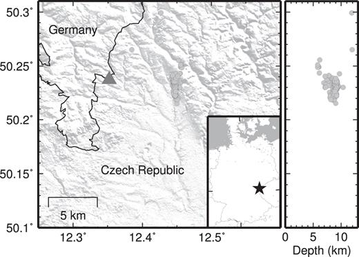
Map of the West Bohemia/Vogtland area at the Czech-German border. Shown is the position of the borehole (triangle). Locations of earthquakes from 2014 June to August with 0 ≤ ML ≤ 1 are plotted as grey dots. A latitude-depth section of the earthquakes is shown on the right.
3 DECONVOLUTION INTERFEROMETRY
We use an interferometric approach that applies deconvolution analysis to either earthquake or seismic noise recordings to decompose the wavefield into up- and downgoing wavefields. DCI is preferred over the more commonly used cross-correlation interferometry (CCI). Newton & Snieder (2012) showed that CCI gives the correct phase but incorrect Fourier amplitudes which results in wrong attenuation estimates. DCI, on the other hand, allows for correct phase and amplitude estimation. Furthermore, as the source spectrum cancels in DCI, it is generally preferable over CCI when measuring attenuation.
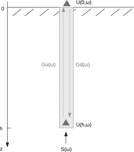
Motions recorded in a borehole due to a vertically incident plane wavefield S(ω) coming from below. U(0, ω) and U(h, ω) are the motions recorded at the surface and within the borehole at depth h. Gu(ω) and Gd(ω) denote Green’s function response due to up- and downward propagating waves, respectively.
4 ESTIMATION OF Q−1(f)
5 DATA ANALYSIS
In a first step, the correct horizontal orientation of the borehole instruments was estimated. The orientation was determined by analysing four teleseismic earthquakes that were recorded at the borehole and the surface station. After the application of a 1 Hz low-pass filter, the borehole traces were sequentially rotated until the best fit with the surface records was obtained. The borehole sensor turned out to be 54.0° ± 0.2° off the horizontal orientation off the surface sensor. In addition, the orientation of the surface instrument was verified with a Gyroscope. A horizontal error of 6.8° was detected. The horizontal components of the surface sensor were, thus, rotated by an azimuth of −6.8°, while the borehole instrument was corrected by 47.2°.
No instrument correction was applied to the data because the borehole and the surface sensor have equivalent responses.
5.1 Intersensor traveltime differences
Traveltimes between the borehole and the surface sensor have to be known in order to compute the quality factor according to eq. (9). For earthquake signals, intersensor traveltimes were estimated for each event by picking P- and S-wave arrivals within the borehole and at the surface. Intersensor traveltimes vary between 0.034 and 0.055 s for P waves and between 0.068 and 0.134 s for Swaves. Computing the arithmetic mean of all values gives 0.043 and 0.085 s for P and S waves, respectively. This leads to a vp of around 2000 m s−1 (ranging between 1580 and 2560 m s−1) and a vs of around 1000 m s−1 (ranging between 650 and 1280 m s−1) between borehole and surface sensor. The mean intersensor traveltime 〈τ〉 of S waves is used for the computation of log-mean |$Q_s^{-1}$| curves (eq. 12).
Seismic waves should reach the borehole instrument with vertical incidence in order for eqs (1)–(4) to be fully valid. We randomly selected earthquakes from the data set that took place at different distances and at different depths. The incidence angles that are deduced from the particle motion of the P arrivals are 28°–42° within the borehole and 14°–25° at the surface.
For noise recordings, we estimated S-wave intersensor traveltimes directly from the mean noise deconvolution time traces in Fig. 3 (left). The two arrivals that are observed in the deconvolved wavefields on the acausal and the causal parts of the trace should be separated in time by 2τ. However, it is not immediately apparent where to set traveltime picks in the deconvolutions. We simply picked the maxima of the acausal and the causal signal arrivals and find an S-wave traveltime of 0.091 s. A similar value is obtained when correcting the mean intersensor traveltime 〈τ〉 obtained from the earthquake recordings to zero incidence angle. Dividing the 〈τ〉 value by the cosine of a mean incidence angle between borehole and surface station of approximately 27° leads to 0.095 s for S waves. This indicates the presence of body waves in the incoming noise wavefield that impinge at the borehole sensor with almost zero incidence angle. Individual 1 hr long noise deconvolutions are very similar to the stacked noise deconvolution time-series (see Fig. 5). We therefore use the same S-wave intersensor traveltime of 0.095 s for the computation of individual 1 hr and log-mean noise quality factors.
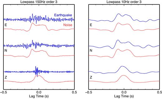
DCI results between borehole and surface sensor computed from ambient noise (red) and from earthquake records (blue) for all three components. Left: deconvolved time traces filtered with a Butterworth low-pass filter of 150 Hz and order 3. Right: traces filtered with a 10 Hz low-pass Butterworth filter of order 3. Note the similarity of noise and earthquake deconvolutions for low frequencies. The colour version of this figure is available only in the electronic version.
5.2 Ambient noise processing
We selected nine full days of data (2014 May 14–22) for the computation of ambient noise deconvolution. These days lie before the start of the Bohemian earthquake activity on 2014 May 24. The 1 hr long noise data were pre-processed by first removing the offset of each trace. Possible transient signals were eliminated by excluding signal windows from the data that have amplitudes larger than an hourly median amplitude level (Zhang & Yang 2013). To do so, we computed for each 5 min long data window the envelope mean. The signal in this window was replaced with zeros if it exceeded two times the median envelope amplitude computed for the whole hour. The traces were then split into 100 s long time windows with an overlap of 50 per cent (Welch’s method, Welch 1967; Seats et al.2012). Windows were tapered at the edges with a 5 per cent cosine taper. The deconvolution was computed following eq. (6). All deconvolved sequences originating from the same 1 hr long data window were stacked.
5.3 Earthquake data processing
We selected earthquakes from the 2014 relocated Webnet catalogue that was used in Hainzl et al. (2016). Only events with 0 ≤ ML ≤ 1 were chosen to avoid complex source time functions and non-linear site responses of the ground. We visually checked each event and removed records if, for example, earthquakes overlapped or if data quality was too bad. All earthquakes occurring in the time span from 2014 May 24 to June 03 had to be omitted due to data logger malfunction of the surface station after a thunderstorm. In total, 194 earthquakes were selected. All earthquakes occurred approximately east of the borehole and close to each other (compare to Fig. 1) at distances between 5 and 12 km (average distance of 10.6 km) and at depths of 6–12 km (average depth of 8.8 km).
We took the whole 4 s long earthquake signal (starting at the P-wave arrival time) for DCI calculation instead of selecting P- and S-wave windows. Mehta et al. (2007) and Parolai et al. (2009) showed that the deconvolutions are insensitive to the chosen signal window and only depend on the component of ground motion that is analysed. P-wave energy is always observed on the deconvolved Z component and S-wave energy on the deconvolved horizontals irrespective of the chosen signal window. We tested this for all earthquakes and made the same observations. Deconvolution results and also Q−1 estimates are similar for selected P- and S-wave windows and for whole earthquake data segments.
The records were processed similar to noise recordings. First, signal offset was removed. The data windows were tapered at the edges with a 5 per cent cosine taper and the deconvolution was computed in frequency domain.
5.4 Deconvolution time-series processing
The time-window length for cutting incident and surface-reflected waves from deconvolutions has to be chosen carefully. Very short time windows cut-off important parts of the signal and lead to lower frequency resolution while windows that are too long include not only signal but also too much noise. We decided to use the same time-window length for noise and earthquakes in order to make the attenuation results better comparable. After testing, a time-window length of 0.3 s (starting or ending at zero lag time for causal and acausal wave arrivals, respectively) was chosen. Cut traces were tapered with a 5 per cent cosine taper before taking the Fourier transform. |$Q_s^{-1}$| was computed from the N and E components and the mean curves were estimated using eqs (9) and (12).
6 RESULTS
Fig. 3 shows the deconvolution results obtained from seismic noise and from earthquake records after stacking over all available 1 hr long noise deconvolutions or single earthquake deconvolutions, respectively. The Z components display P-wave energy travelling with faster velocity than the Swaves that are visible on N and E. Deconvolution from earthquake records is richer in higher frequencies which is also visible in the deconvolution amplitude spectra of Fig. 4. Amplitudes of noise deconvolutions start to decrease above 6 Hz while the amplitude of earthquake deconvolutions remains high. Deconvolution results derived from noise and earthquakes are very similar for low frequencies as is shown in Fig. 3 (right).

Fourier amplitude spectra of the deconvolution results shown in Fig. 3 (left). Background noise spectra were taken from the first and last 1 s of the in total ±10 s long noise deconvolution time-series’. The colour version of this figure is available only in the electronic version.
Fig. 5 summarizes the low-pass filtered deconvolutions of each of the 1 hr long noise segments and each of the 194 earthquake records, respectively. The results are very similar for different noise windows. There are larger variations between individual event deconvolutions.
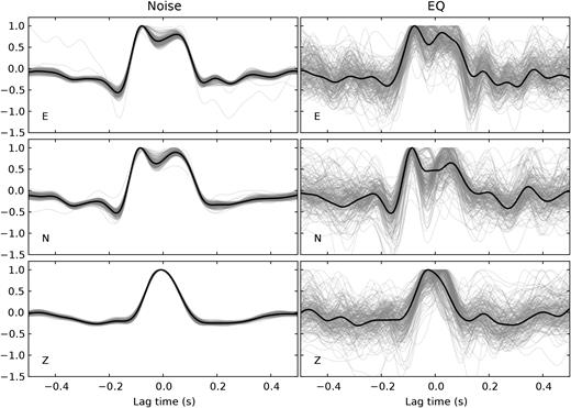
Deconvolution results for seismic noise (left) and earthquake recordings (right) for all three components of motion ZNE. Thin traces show the results of each of the 1 hr long noise segment or of each of the 194 events, respectively. Black lines are stacked results. Traces are filtered with an acausal Butterworth low-pass filter of 10 Hz and order 3. Each trace is normalized to its maximum.
Up- and downgoing P waves are badly separated in the deconvolution traces of the Z component. We therefore do not use the Z component in the further analysis and focus on the estimation of |$Q_s^{-1}$| from horizontal motions only. Fig. 6 shows the transfer functions computed with eq. (7) from noise DCI (left) and earthquake DCI (right). Thin grey lines are transfer functions derived for different 1 hr long noise windows or different earthquakes, respectively. The thick solid and dashed blue lines represent the log-mean ±1 standard deviation of all grey T(f) curves computed according to eqs (10) and (11). Individual one hour long noise T(f) responses are fairly consistent below approximately 15 Hz. Above 15 Hz, the results show larger variations. This behaviour is represented by small standard deviations of the log-mean curves below 15 Hz and larger standard deviations above this frequency. The differences between single earthquake T(f) curves are generally high as is the standard deviation of the log mean.
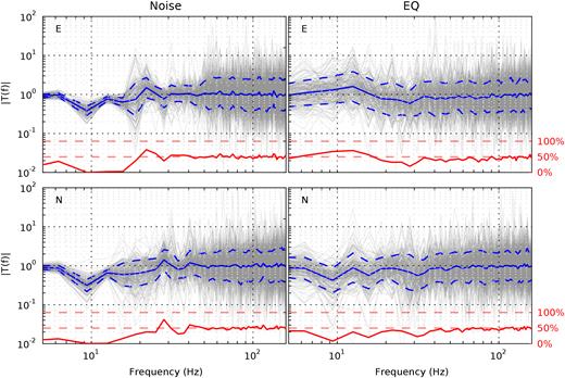
Transfer functions computed from noise DCI (left) and earthquake DCI (right). N components are displayed at the bottom and E at the top. Thin grey lines are transfer functions for individual 1 hr long noise windows or single earthquakes. The blue line is the logarithmic average of all transfer functions. Blue dashed lines show ±1 standard deviation. Red lines of the bottom of each panel show the percentage of transfer functions with T(f) > 1. The colour version of this figure is available only in the electronic version.
The red line at the bottom of Fig. 6 displays the percentage of data points with T(f) > 1. A value of T(f) > 1 will lead to a |$Q_s^{-1}\lt 0$| and therefore to an amplitude increase instead of attenuation. Most of the noise transfer functions are smaller than one at frequencies below 15 Hz. The amount of curves with T(f) > 1 is around 50 per cent at higher frequencies. On the contrary, many transfer functions derived from earthquakes have values larger than one irrespective of the chosen frequency range.
Fig. 7 shows |$Q_s^{-1}(f)$|. As in Fig. 6, thin grey lines are computed for individual 1 hr long noise windows or different earthquake recordings, respectively. The blue lines are computed from the log-mean T(f)′s. Because axes are plotted logarithmically curves are interrupted or not shown if |$Q_s^{-1}\lt 0$|.
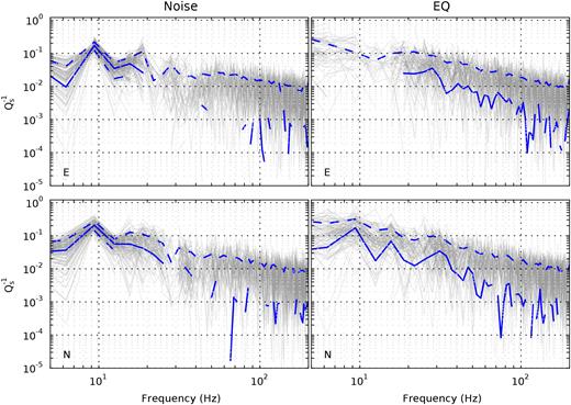
Frequency-dependent |$Q_s^{-1}$| computed from noise DCI (left) and earthquake DCI (right). |$Q_s^{-1}$| derived from N and E components are shown at the bottom and at the top, respectively. Thin grey lines are |$Q_s^{-1}$| estimates calculated for individual 1 hr long noise windows or single earthquakes. The blue line is computed from the log-mean transfer function shown in Fig. 6. Blue dashed lines show ±1 standard deviation. Curves are interrupted if |$Q_s^{-1}\lt 0$|. The colour version of this figure is available only in the electronic version.
The log-mean curves of |$Q_s^{-1}$| (all blue curves in Fig. 7) are summarized in Fig. 8 for the frequency range 5–20 Hz. |$Q_s^{-1}$| obtained from the E component of earthquakes are negative within this frequency range and are therefore not shown. Noise- and earthquake-based |$Q_s^{-1}$| estimates are within the same order of magnitude.
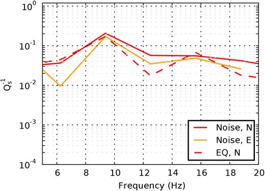
Comparison of |$Q_s^{-1}$| estimates (blue lines in Fig. 7) for frequencies between 5 and 20 Hz. Abbreviation: EQ = earthquake. The colour version of this figure is available only in the electronic version.
7 DISCUSSION
With DCI, it is possible to observe the separation of the wavefield into incident and surface-reflected P and S waves in the West Bohemia/Vogtland area. This is not only possible with earthquake recordings but also with seismic noise. The stack in Fig. 3 was performed over nine full days of noise data. However, deconvolution of only a single 1 hr long noise trace is sufficient to obtain a clear result (compare to Fig. 5). The situation is different for earthquake recordings. Earthquake deconvolutions have a higher frequency content than noise deconvolutions and the separation into incident and surface-reflected waves is not as clearly visible as for seismic noise without low-pass filtering. Furthermore, up- and downgoing waves are only stable visible in the deconvolved earthquake traces when stacking over a sufficient number of events.
The transfer functions shown in Fig. 6 reveal a very similar pattern. The transfer function computed from a single 1 hr long noise deconvolution resembles the mean T(f) of all noise segments very well at frequencies below 15 Hz. At higher frequencies, noise T(f) curves are very different because the amplitude level of the noise deconvolution is almost at the same level as the amplitude of the background noise (Fig. 4). Transfer functions of earthquake recordings, on the contrast, vary strongly. This overall behaviour of curves can also be observed for noise- and earthquake-derived |$Q_s^{-1}$| measures shown in Fig. 7.
The red percentage line in Fig. 6 can be regarded as a quality measure for the interpretation of log-mean transfer functions and |$Q_s^{-1}$| estimates. Mean |$Q_s^{-1}$| curves will be reliable for frequencies where only a small percentage of transfer functions is above one. This is the case for seismic noise below 15 Hz. Mean earthquake |$Q_s^{-1}$| measurements have to be taken with more care as many single-event |$Q_s^{-1}$| estimates are below zero and therefore drag the log-mean curve to smaller |$Q_s^{-1}$| values. This is especially true for the E component below 15 Hz where the red line in Fig. 6 shows that more than 50 per cent of the curves have values of T(f) > 1. As a consequence, |$Q_s^{-1}$| cannot be recovered from the E component of earthquakes at low frequencies (compare to Figs 7 and 8).
One possible reason of the inferior performance of earthquake compared to noise recordings may be attributed to the non-zero incidence of earthquake waves. The assumption that the reflection coefficient at the free surface is one and that the free-surface factor is 2 is violated for waves that do not arrive steeply from below. This will affect the amplitudes of the causal and acausal wave arrivals in the deconvolved seismograms. In addition, SV–P conversions occur at non-zero incidence between the P- and the S-wave arrival and can further influence the amplitude of the downward reflected wave in the radial direction of motion. All earthquakes are located approximately east of the borehole so that the E component corresponds roughly to the radial direction whereas the N component coincides with the transverse direction. SV–P conversions are thus expected to affect mainly the amplitudes of the reflection on the E component. This may be the reason why we are not able to recover |$Q_s^{-1}$| for the E component of earthquakes at frequencies below 15 Hz. Mean DCI results, T(f) and |$Q_s^{-1}$| curves estimated from the N component of earthquakes are, however, very similar to noise-derived curves.
Up- and downward propagating waves partly overlap in the deconvolution traces obtained from seismic noise or from earthquakes. We performed numerical simulations (see Appendix) in order to evaluate the influence of the insufficient signal separation on the estimation of Qs−1. The results reveal that Qs−1 can also be recovered for shallow depths and for partially overlapping incident and surface-reflected waves in the deconvolution traces. Problems arise only at low frequencies were Qs−1 is overestimated. In addition, the scatter around the true value of Qs−1 is larger for shallower borehole recordings and improves as the sensor depth increases. The fluctuation of Qs−1 observed in Fig. 8 thus might be an effect of shallow borehole depth.
The deconvolution of noise recordings leads to very clear body wave signatures. Seismic noise is considered to be dominated by surface waves below 1 Hz, while at higher frequencies, the noise wavefield is suspected to be a mix of body and surface waves (Bonnefoy-Claudet et al.2006). According to theory, the coherent noise sources contributing to the deconvolution have to be situated along the interstation direction of the sensors, the so-called end-fire lobes (Roux & Kuperman 2004; Snieder 2004). Sources outside the end-fire lobes interfere destructively if distributed homogeneously. Due to the strong impedance contrast at the free surface no significant amount of noise energy is assumed to enter the ground from above. This is confirmed by the observation that the deconvolved time-series’ are acausal and two-sided which is only the case if the incoming noise wavefield approaches the borehole from below (Snieder 2009). Part of the seismic noise therefore needs to come from below the borehole station and cannot be explained by surface waves in the noise field. The amplitude spectra obtained from noise and earthquake deconvolutions as shown in Fig. 4 have a very different frequency content. Local events of very small or negative magnitude that may be present in the noise wavefield can therefore be ruled out as possible source of the body waves. One possible explanation for the presence of body waves in the noise wavefield might be scattering conversions at subsurface heterogeneities. Body waves could also be generated by local surface sources (e.g. close-by cities or roads) and arrive at the borehole sensor as diving waves from below. This was, for example, observed in a noise cross-correlation study of Hillers et al. (2012) at the Taiwan Chelungpu-fault Drilling Project (TCDP) borehole in Taiwan. Hillers et al. (2012) identified a cultural origin of body wave noise that follows the trajectory of a ballistic wave through the subsurface and enters at the borehole as coherent upward propagating body wave noise between 1 and 16 Hz. The origin of body wave noise in the West Bohemia/Vogtland may be a topic for future research.
The quality factors that are estimated within this study can be interpreted as effective ones including both, intrinsic and scattering attenuations. Eulenfeld & Wegler (2016) separated intrinsic and scattering attenuations of seismic shear waves by envelope inversion of local earthquakes in the Vogtland area. They found a scattering Qs of 166–3000, an intrinsic Qs of 100–2500, and a total Qs of 67–1600 between 1 and 50 Hz. The Qs values reported by Eulenfeld & Wegler (2016) were obtained for the whole travel path between source and site and are therefore higher than the near-surface values computed in this study. Nevertheless, their results reveal that scattering attenuation cannot be neglected in the Vogtland area. A superposition of intrinsic and scattering mechanisms thus might explain the amplitude decay between incident and surface-reflected waves.
Qs varies around a value of 20 between 5 and 20 Hz with a minimum value of 5 and a maximum value of 100. Typical Q-values in the lithosphere are reported to be of the order of 102–103 in the frequency range 5–20 Hz (Sato et al.2012, fig. 5.1). Our results are, however, in conformance with attenuation measurements conducted at the KTB (Continental Deep Drilling Project) that is situated approximately 50 km to the southwest of the study site and that was drilled in a very similar crystalline environment down to a depth of about 9000 m. Li & Richwalski (1996) found Qs to be between 8 and 25 at depth of 3–6 km and for frequencies between 11 and 22 Hz. Müller & Shapiro (2001) concluded that scattering attenuation plays an important role at the KTB site and might explain the low effective Q estimates. Several other borehole studies conducted at different rock sites of the world reported similarly high effective attenuations for depths shallower than 3 km (e.g. Aster & Shearer 1991; Abercrombie 1997, and references therein).
A comparison of our results with studies that employ the DCI method to earthquake recordings is only partly possible because these studies are usually conducted at sedimentary sites. Raub et al. (2016) obtain a Qs of 20 between 0 and 288 m depth and at frequencies of 0.1–40 Hz in a limestone formation. Parolai et al. (2010) derive an average Qs of about 30, 46, and 99 for the 0–50, 0–70, and 0–140 m depth ranges, respectively, between 1 and 20 Hz for a site structure that is composed of limestone, clayey sand, and sandstone layers.
The low Qs estimates of our study are supported by slow P- and S-wave velocities that we observe between 0 and 87 m depth (compare to Section 5.1). The phyllites and mica schists are reported to be weathered up to at least 40 m depth (personal communication with BBM) which can certainly lead to low seismic velocities and high attenuation. As to our knowledge, there are no other studies in the area that investigate attenuation at similar depths and at similar frequencies as in our study.
8 CONCLUSION
We apply DCI to seismic noise recorded in a borehole configuration. We show that up- and downgoing waves are well observed in the deconvolved traces despite the fact that noise recordings are usually assumed to be mainly composed of surface waves. Only short noise segments are necessary to obtain stable deconvolution results. DCI with ambient noise is thereby advantageous over DCI using earthquake recordings where several events are required to obtain a stable deconvolution. In addition, earthquake deconvolutions suffer from the non-zero incidence of earthquake waves so that |$Q_s^{-1}$| can only be recovered for the transverse component of motion due to P–SV conversion. On the contrary, |$Q_s^{-1}$| estimation from the deconvolution of seismic noise is limited to frequencies below 15 Hz in the West Bohemia/Vogtland area, whereas earthquake deconvolutions are richer in higher frequencies. More research is needed to prove that DCI using ambient noise recorded in a borehole is also applicable to other areas or if the presented method is only valid if, for example, scattering attenuation is high. Furthermore, the origin of body waves in the noise wavefield needs to be investigated.
We are able to extract frequency-dependent quality factors for S waves between 5 and 15 Hz. The obtained quality factors are very small (Qs ≈ 20) but are in agreement with the results of other borehole studies conducted throughout the world. Available borehole logging information tells that the rock at the study location is weathered down to 40 m depth. This is probably the main reason for the low velocities and the high attenuation that we observe.
The presented method has the ability to provide an easy tool for the extraction of quality factors in the near-surface if borehole recordings are available. This is especially the case for low- and mid-seismicity regions where earthquake recordings are sparse but where subsurface information is needed to assess, for example, the seismic hazard. The procedure may also be useful for continuous time-lapse monitoring of seismic velocity given the fact that a very short duration of ambient noise seems to suffice to obtain stable deconvolution results. Ambient noise interferometry thus provides a suitable alternative to earthquake-based borehole methods.
ACKNOWLEDGEMENTS
The borehole is operated by Bad Brambacher Mineralquellen (BBM) GmbH & Co. Betriebs KG. We are very thankful to the BBM to make this borehole available for seismological studies. We owe further thanks to the GFZ German Research Centre for Geosciences Section 2.1 for logistical support and help during the field work. Deconvolution and seismological data analysis were done using ObsPy, a Python framework for seismology (Beyreuther et al.2010), and with the MIIC library (https://github.com/miic-sw/miic, last accessed 2015 October 01) that emerged from a project called Monitoring and Imaging based on Interferometric concepts. Some plots were made using Generic Mapping Tools (GMT) version 4.5.6 (Wessel & Smith 1998). We are grateful to Tomá#x0161; Fischer for providing the Webnet catalogue with relocated events. QSEIS can be obtained from https://www.gfz-potsdam.de. The first author of this publication was partly funded by the section for equal opportunity of the Faculty of Science, University of Potsdam. She is furthermore a member of the Helmholtz graduate research school GeoSim. We are very grateful to the two anonymous reviewers who gave valuable suggestions and comments which led to an improvement of the manuscript.
REFERENCES
APPENDIX: NUMERICAL TESTS
The causal and acausal signal components partially overlap in the deconvolution traces. We conducted numerical tests in order to study the influence that this overlap can have on the estimation of |$Q_s^{-1}$|.
We used QSEIS (Wang 1999), a code that employs the orthonormal propagator algorithm, to compute synthetic seismograms for a viscoelastic 1-D subsurface model. According to the results obtained for the West Bohemia/Vogtland area within this study (Section 5.1), vp and vs were set to 2000 and 1000 m s−1, respectively, and Qs was chosen to be 20. A source was placed at 4.2 km depth on an arbitrarily chosen fault plane with a strike, dip, and rake of 170°, 75°, and −30°, respectively. Synthetic seismograms were calculated for receivers that are placed at the surface and at different depths (50–500 m) directly above the source. White noise with 10 per cent of the maximum amplitude was added to the synthetics. We applied the same procedure to the synthetics as to the real data by first computing the deconvolution with respect to the surface sensor according to eq. (6). Epsilon had to be set to 0.1 in order to obtain stable deconvolutions. |$Q_s^{-1}$| was then derived using eq. (9). The results are shown for the transverse component of motion.
Fig. A1 shows the deconvolutions obtained for borehole receivers at depths of 50, 87, 100, 200, and 500 m. At shallow depths, the causal and signal components partially overlap.
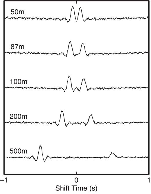
Deconvolution traces obtained from synthetic seismograms that were computed using QSEIS. Shown is the transverse component and the results for different sensor depths after deconvolution with the motion recorded at a surface sensor.
Fig. A2 summarizes the |$Q_s^{-1}$| results that are obtained for different sensor depths. The input |$Q_s^{-1}$| of 0.05 can be recovered for frequencies between 1 and 12 Hz. The result is most clear for the deepest sensor at 500 m. For shallow receivers, the results tend to fluctuate around the true |$Q_s^{-1}$| value. |$Q_s^{-1}$| is overestimated at frequencies below 6 Hz for the receiver at 50 m depth. This might be caused by the insufficient causal and acausal signal separations at shallow depth which will be most prominent at low frequencies.
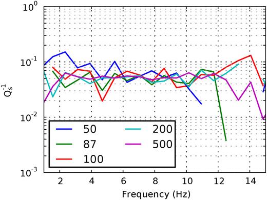
|$Q_s^{-1}$| that is obtained from the deconvolution traces shown in Fig. A1. The sensor depth is colour coded.
