


SUMMARY
This paper focuses on the combined analysis and interpretation of controlled source electromagnetic (CSEM) and multichannel reflection seismic (MCS) data along one profile in the German North Sea with the goal to reduce ambiguities in interpretation. The shallow water environment of the North Sea is characterized by a complex geological development which includes rifting, several ice age cycles, a propagating shelf margin, mass-transport deposits and salt dome formation. Seismic and electromagnetic methods are sensitive to different physical properties of the seabed and therefore complement each other. We analyse the MCS data with a migration velocity tomography and an amplitude variation with offset analysis and discuss seismic velocities and densities. For true amplitude recovery the amplitude distortions are calibrated with in situ logging data. The CSEM data are analysed in 2-D, for which, for the first time, data were included that were acquired while the instrument was towed on the seafloor in addition to the stationary sites. The CSEM inversions are constrained by seismic horizons. The joint interpretation focuses on two seismic reflectors: One can be interpreted as an unconformity marking a lithological change from fresh water-bearing glacial deposits to compacted sediments below, and the other one as a layer of fine-grained deposits potentially capping patchy shallow gas occurrences. This exemplary case study shows how the combination of both methods can benefit by interpreting complex geology and eliminating ambiguous explanations.
1 INTRODUCTION
Geophysical methods provide the scientific community with an opportunity to study the subsurface remotely by exploring its physical properties down to great depth that is too expensive to drill. The physical properties are interpreted in relation to the geology of the subsurface, which may be ambiguous given certain geological formations have similar physical properties. It is therefore beneficial to combine different geophysical methods with focus on their different physical parameters in order to gather unambiguous geological information about the study area. In this case study, we combine marine controlled source electromagnetic (CSEM) and multichannel reflection seismic (MCS) data to study a 2-D section of the German North Sea (see Fig. 1) down to several 100 m depth. This work is linked to the project Geo-scientific Potential of the German North Sea (GPDN).
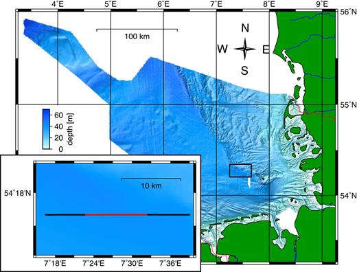
Bathymetry of the German sector of the North Sea (http://www.gpdn.de) with survey area (black rectangle) located North West of Heligoland in the Elbe palaeovalley. Inlay: Survey area with CSEM profile (red) and MCS line AUR03-23a (black); water depth along the profile is about 41 ± 0.5 m.
The two methods are sensitive to different physical parameters and can complement each other in interpretations of the subseafloor geology. The active seismic method, for example, is sensitive to impedance contrasts and therefore resolves structural changes, but is poor at detecting gradual changes within the sediment volume. Furthermore, strong seismic impedance contrasts transmit relatively little seismic energy down to greater depths. Small amounts of free gas already cause strong impedance contrasts, but a further increase in gas concentration has only little effect on the resulting reflection pattern (Domenico 1976). The CSEM method, in comparison, is more sensitive to bulk volume changes in resistivity, and different levels of pore space occupation with resistive material (e.g. free gas) are differentiable (Constable 2010). Combining the two techniques reduces ambiguities in the interpretation of features from the individual analysis alone.
1.1 Reflection seismic data
The MCS profile AUR03-23a (Kudraß et al.2003) has been acquired in 2003 from the privately owned motor vessel MV AURELIA using a GI-Gun (harmonic mode) with generator and injector volumes of 25 cu in each and a streamer towed at 4-m water depth with an active length of 300 m and 24 hydrophone groups. The shot point interval was about 12.5 m. Zero-offset seismic reflection data are sensitive to the impedance contrasts (product of seismic velocity and density) and have a high resolution even at greater depth, depending on the frequency content and amplitude of the source signal. The recorded maximum offset of 312 m and the shallow water depth enable analysing the seismic velocities and further the amplitude variation with offset (AVO) characteristics of subseafloor reflectors down to a depth of about 270 m using reflection angles up to 30°. After applying a calibration technique to correct for true amplitudes, we perform an AVO analysis, and finally model seismic shear wave velocities to investigate two pronounced reflectors.
1.2 Controlled source electromagnetic data
The marine CSEM data have been acquired with a seafloor-towed array developed at the German Federal Institute for Geosciences and Natural Resources (BGR; Schwalenberg & Engels 2011; Schwalenberg et al.2012). It consists of a horizontal current source dipole and four electric receiver dipoles. The method is based on electromagnetic field diffusion from the source to the receivers. The measured electric field amplitudes and traveltimes depend on the electrical resistivity, or its reciprocal the conductivity, of the subseafloor and the seawater. Due to the diffusive character of the field propagation, the solution to the subseafloor resistivity structure is always non-unique, and sensitivity to the subsurface structure reduces with distance and target depth. However, CSEM data analysis results in reliable bulk estimates of the subsurface resistivities. The bulk resistivity of marine sediments is mainly controlled by conductive pore water, and resistivity contrasts relate to changes in porosity, pore water conductivity, permeability and hydrocarbon content among other factors (Edwards 2005; Constable 2010). The marine CSEM method has become a popular tool to detect electrical resistivity contrasts in the seabed that may relate to potential hydrocarbon reservoirs (e.g. Constable & Srnka 2007).
The CSEM data of the study area have previously been analysed in time domain with a 1-D Bayesian inversion technique including the number of the parameters as an unknown in the inversion (Gehrmann et al.2015), and a combination of a linearized and non-linear 1-D inversion techniques introducing lateral constraints (Moghadas et al.2015) to study the resistivity distribution and its uncertainty. Gehrmann et al. (2015) have shown that resistivities can be well resolved to about 300 m depth (about half of the source–receiver offset), and that resistivities respond to the differing geology of Holocene, Pleistocene and Miocene sediments.
In this paper, we present frequency-domain 2-D inversion results obtained with a linearized technique (code MARE2DEM by Key 2016). Data analysis in the time or frequency domain theoretically yields the same information, but practical differences exist due to the amount of data selected for processing, the use of different sources and differing noise levels (e.g. Cheesman et al.1987; Connell & Key 2013). Therefore, a large range of frequencies is selected to match the data range of the time-domain analysis. For the purpose of providing a denser data coverage for the 2-D analysis, additional CSEM data have been analysed not only when the seafloor instrument was stationary [as presented in Gehrmann et al. (2015) and Moghadas et al. (2015)], but also for the first time while the bottom-towed instrument was moving (max. 1 kn), so called roll-on data. Furthermore, the inversion of this study included structural constraints from the reflection seismic data that have been identified in Gehrmann et al. (2015) with the purpose to relate to the same geological boundaries.
2 SEISMIC DATA ANALYSIS
Seismic energy travels through media in the form of seismic elastic waves, which comprise compressional (P) waves and shear (S) waves. Media are characterized by their seismic impedance, the product of P-wave velocity VP and density ρ. The amount of zero-offset reflected seismic energy at a boundary between two media directly relates to the impedance contrast, which means it depends on VP and ρ only. However, the offset-dependent amplitude variation for a reflected wave mainly relates to the contrast in S-wave velocity (Castagna & Smith 1994). Therefore, an AVO analysis can deliver an additional parameter to describe changes in physical parameters across a layer boundary. The amplitude behaviour with respect to different incident angles at a reflector is theoretically described by the four Zoeppritz equations (e.g. Aki & Richards 1980). They describe the reflected and refracted P- and S-wave amplitudes at an interface as a function of angle of incidence, density and seismic velocities.
The seismic energy is attenuated while it is travelling through the media because of geometric spreading proportional to the distance away from the source, intrinsic attenuation due to internal friction and transmission losses due to diffraction (Mondol 2010). An amplitude-dependent analysis such as the AVO method requires correcting for amplitude attenuation. Here, we present a method of calibrating the seismic amplitudes with in situ logging data.
2.1 Seismic data processing
To obtain a first structural image along line AUR03-23a standard processing is performed including a bandpass filter with pass band between 50 and 180 Hz. Since a precise knowledge of the seismic velocity distribution at depth is essential for the AVO analysis, we applied a multistep velocity analysis. The first step involved a classical normal moveout semblance analysis on super gathers. In a second step, the velocity analysis was combined with a pre-stack depth migration velocity analysis (MVA). The residual moveout was analysed on the pre-stack migrated gathers and the velocity model was revised from top to bottom via a layer-stripping approach. Finally, we refined the velocities for the whole profile using MVA tomography, taking into account the residual moveout for all horizons simultaneously. Seismic interpretation in the sediment regime is typically done in time sections (e.g. Fig. 2), however, models for interpretation are presented as depth section (e.g. Fig. 9) after pre-stack depth migration using the final tomography velocity model. To account for amplitude loss due to spherical wave front spreading, a spherical divergence correction was applied using the resulting velocities. After stacking the data, a predictive deconvolution was performed to suppress multiple reflections from the seafloor. The resulting stacked section is shown in Fig. 2. The seismic section shows two pronounced reflectors. The upper reflector, upR, is situated at a depth between 140 and 190 ms two-way traveltime (TWT) with a slight dip to the east. It shows the same polarity as the seafloor. The lower reflector, loR, is a flat structure at depth of around 310 ms TWT. The polarity of this reflector is reversed, therefore it represents a negative impedance contrast.
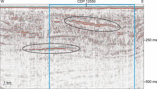
Stacked section of line AUR03-23a (black line in Fig. 1). This profile is characterized by two pronounced reflections, marked with ovals. In the following we refer to this as the upper reflector upR and the lower reflector loR, respectively. Also shown is the common depth point location (12550) where AVO modelling was performed for the upper reflector (see Section 2.2). The window were the CSEM profile overlaps with the seismic profile is marked with a blue frame.
2.2 Calibration of seismic amplitudes and AVO analysis
To deduce reflection coefficients from measured seismic amplitudes, we have to apply several corrections. Based on the geological conditions of the area under investigation, in the only partly consolidated sedimentary column close to the surface, the dominant factor influencing the amplitude decay should be spherical divergence (O’Doherty & Anstey 1971). If the velocity distribution within the subsurface is known, the effect of divergence should be easily compensated (Newman 1973). Therefore, we applied a time and velocity dependent spherical divergence correction to the pre-stack data. A second major source for amplitude distortion might be the radiation pattern of the source as well as the directivity of the receiver. The amplitude dependence on the directivity of a similar source configuration (GI gun towed at a depth of 3 m) and the effects between source and surface of the sea have been analysed by Zillmer et al. (2005). Here, the seismic receivers within the streamer are summed up over a distance of 12.5 m. Therefore, an angle-dependence of the recorded amplitude can also be expected. Since the combination of both effects cannot be estimated properly, we decided to calibrate the offset-dependent amplitude distortion with the help of a drilled horizon on another seismic line from the same survey.
The seismic line AUR03-22 from the same survey (Kudraß et al.2003) crosses a drill site (R1, Thöle et al.2014) at about 100 km to the north of AUR03-23a. At depth of about 270 ms TWT, logging at the drill site reported a lithological transition from sediments with sandy gravel to silty clay. To predict the AVO characteristics at this interface, the Zoeppritz’ equations are solved using the following parameters: The P-wave velocities from the detailed MVA tomography (VP1=1900 m s−1 for the upper layer and VP2 = 2075 m s−1 for the lower layer) and the corresponding densities (ρ1 = 2046 kg m−3 and ρ2 = 2092 kg m−3, following Gardner et al.1974). Concerning the S-wave velocity, a two-step procedure was followed: The gamma-ray log was used to calculate clay content for both layers following Rider (1996). The clay content was related to VS following the work of Han et al. (1986) delivering VS1 = 870 m s−1 and VS2 = 950 m s−1. The resulting VP/VS ratios for both layers are about 2.2, which are reasonable values for uncemented sediments (Mavko et al.1998).
The extracted amplitudes for the reflector at line AUR03-22 were plotted against the solution of the above described Zoeppritz’ equations, and resulting correction factors were estimated for all channels. As a result, the far-offset channels have to be corrected by a factor of about 3 compared to the near-offset channels. This value seems reasonable given the angle dependence of the directivity of the source and the receivers.
After correction of all traces for line AUR03-23a, we performed a classical AVO analysis following Shuey’s approximation (Shuey 1985). He postulated that the zero-offset reflectivity can be described by the AVO intercept A, while the angle dependent reflectivity R(θ) depends on Bsin2(θ), where B is the AVO gradient and θ the reflection angle. A basic tool for analysing A and B is crossplotting (Castagna & Svan 1997). The crossplot for both horizons marked in Fig. 2 as well as the background trend are shown in Fig. 3.
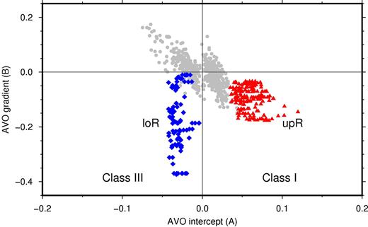
Crossplot of extracted AVO-parameters for the upper reflector upR in Fig. 2 (red triangles), lower reflector loR (blue diamonds) and the background trend (grey dots). Reflector upR shows a reasonable clustering with positive intercept and negative gradient, while reflector loR is characterized by a large range of measured AVO gradients. The AVO classes I and III are defined in Castagna & Svan (1997).
2.3 Amplitude variation with offset modelling
To perform a further analysis of the physical properties causing the shallow reflector upR, peak amplitudes were extracted on prestack data, and an appropriate Zoeppritz solution to this reflection pattern was found. This is a valid approach in the case of well-known P-wave velocities (e.g. Schnabel et al.2007).
The analysis around common depth point (CDP) 12550 (see Fig. 2) is presented here. Since reflector upR shows a laterally stable behaviour (see clustered red dots in Fig. 3), we averaged its extracted peak amplitudes over all CDPs for each channel individually on 101 CDP locations (corresponding to a lateral extent of 625 m). This reduced the effect of scattering. Based on the depth of the reflector, each offset was transformed to a reflection angle. The calibrated amplitudes are shown as circles in Fig. 4. To solve the Zoeppritz’ equations, following parameters were used: The P-wave velocity for the layer above reflector upR VP1 = 1620 m s−1 and for the layer below upR VP2 = 1800 m s−1 were extracted from the MVA tomography, and the resulting densities ρ1 = 1966 kg m−3 and ρ2 = 2019 kg m−3 were estimated using Gardner et al. (1974). To describe the S-wave velocity in the upper layer, we applied an empirical relationship from Hamilton (1976), which delivered VS1 = 397 m s−1 for a depth of 130 m. The S-wave velocity for the lower layer was derived by fitting the Zoeppritz solution to the measured amplitudes resulting in VS2 = 640 m s−1. The modelled amplitudes are shown as a solid line in Fig. 4.
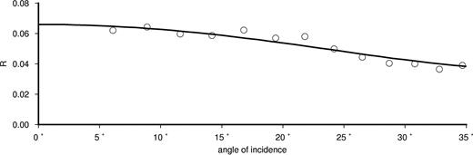
Calibrated amplitudes of reflected P-wave versus angle distribution for the upper reflector upR (open circles). The amplitudes were scaled to the theoretical reflection coefficient R0 at zero offset, based on the P-wave velocities and densities used for the modelling. The solid line represents the corresponding solution to the Zoeppritz equations.
2.4 Result and discussion of seismic analysis
The AVO analysis of two pronounced reflectors delivered some insight into the geological conditions. Possible reasons for the recorded reflection pattern are discussed here. Reflector upR is characterized by a positive intercept A and a negative gradient B (see red dots in Fig. 3). According to Castagna & Svan (1997) this represents the AVO class I. The modelling (Fig. 4) resulted in a VP/VS ratio for the layer above upR of 4.0, while the VP/VS ratio was estimated to be 2.8 for the layer below upR. This points towards a reduced porosity within the underlying strata. The reflector upR represents an unconformity hypothesized to be a buried tunnel valley that was later on filled with glacial deposits. Stewart et al. (2013) and Lutz et al. (2009) present detailed examples of tunnel valleys within the North Sea.
The lower reflector loR shows a negative AVO intercept and also a negative AVO gradient. While reflector upR preserves relative constant AVO gradients along the whole reflector, a much higher scatter is observed for loR. Therefore, no representative Zoeppritz solution could be found for this boundary. Reflectors with negative AVO intercept and negative AVO gradient are generally called AVO class III. Shuey (1985) has shown that a pronounced negative AVO gradient for a class III boundary is caused by the decreased Poisson ratio in the underlying strata compared to the overburden. Further on, Rutherford & Williams (1989) have demonstrated that gas sands could easily produce class III anomalies. The high scatter of the AVO gradient could be interpreted as a patchy distribution of some gas within the sediments.
The geological interpretation based on Thöle et al. (2014) of the seismic section (Fig. 2) is shown on Fig. 5 with major unconformities for the Holocene base, within the Pleistocene (upR) and Tortonium (loR, late Miocene) as well as the Mid-Miocene Unconformity (MMU). The Holocene sediments are assumed to be mainly fine-grained marine deposits, while the Pleistocene sediments are thought to be compacted coarse-grained, unsorted and glacial deposits. Tortonium (late Miocene) deposits are likely to be fine-grained floodplain deposits.
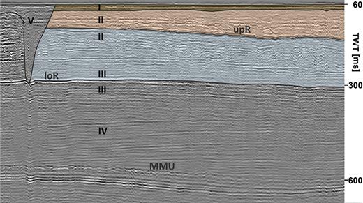
Geological interpretation after Thöle et al. (2014) of the main features and seismic horizons of AUR03-23a. A deep tunnel valley (V) on the left has cut into the late Miocene sediments. The Holocene (I) base is just 20 ms below the seafloor. The shallow reflector upR corresponds to an unconformity within a section of Pleistocene (II) sediments. Pleistocene sediments consist of only few continuing reflectors, while Miocene (III, IV) sediments consist mainly of parallel layers. The lower reflector loR can be associated with the Tortonium (III, late Miocene) and the Mid Miocene Unconformity (MMU) shows its typical polygonal-fault pattern.
3 CONTROLLED SOURCE ELECTROMAGNETIC DATA ANALYSIS
The marine CSEM method typically uses a range of relatively low frequencies between 0.1 and 103 Hz to allow penetration through sea water into marine sediments, and to keep the spatial decay small. The CSEM method is based on electromagnetic diffusion as the electrical conductivity of common earth materials are larger than the product of electric permittivity and frequency. The electromagnetic wave equation is then dominated by the wave attenuation term (conduction currents are larger than displacement currents; Ward & Hohmann 1988), which explains the limitation in penetration depth and structural resolution compared to seismic reflection methods. The CSEM data in this study were acquired with the horizontal inline electric dipole-dipole technique, which is generally preferred compared to broadside source configurations in marine CSEM for its better vertical resolution and sensitivity to resistive layers (Cox 1980; Edwards 2005; Key 2009).
3.1 Instrumentation and data processing
The CSEM array used here (see Fig. 6, Schwalenberg et al.2012) is a seafloor-towed horizontal electric dipole-dipole system. It consists of a 100-m-long transmitter dipole (Tx) and four receiver dipoles (Rx) connected by rope at offsets of 150, 252, 453 and 754 m measured between the centres of Tx and the respective Rx. A heavy weight, called ‘pig’, is towed at the front end of the seafloor array. It contains the transmitter unit (Mir 2011) and a control unit recording the transmitter signal. It also carries an ultrashort baseline Posidonia transponder and a conductivity, temperature and depth (CTD) probe. The CTD probe did not record during the profile presented here, but water resistivities were measured before and after the profile with two vertical CTD profiles. These CTD profiles show resistivities of 0.2315 ± 0.0002 Ωm (Schwalenberg et al.2012).
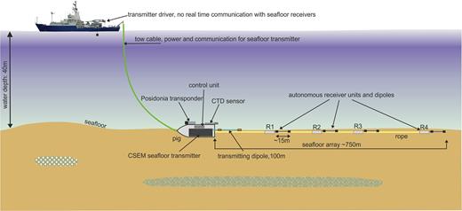
In operation a square wave signal with a maximum amplitude of ±50 A and 6 s period was generated and injected by the Tx into the seafloor and ambient seawater using 1 m copper pipes at each end of the dipole. Each receiver unit consists of an autonomous, battery powered and continuously recording data logger followed by a ∼15 m-long electric dipole with non-polarizable Ag/AgCl electrodes at each end. Data are recorded using a 24 bit analogue-digital converter and a high sampling rate of 10 kHz which allow signal resolution below ∼10 nV. Precise timing between the transmitter and individual receivers is ensured using chip-scale atomic clocks.
The up to 800-m-long array was towed at a low speed of maximum 1 kn along a straight profile through muddy sediments using an approach of about 2 km before the start of profile. Towing on flat seafloor we assume that the receiver dipoles are aligned in line behind the transmitter. During surveying the array is kept stationary every ∼500 m for about five minutes at each measurement site (way point, WP).
The stationary data at the WPs have been analysed in 1-D by Gehrmann et al. (2015) and Moghadas et al. (2015). However, a rigorous 2-D analysis requires a continuous data coverage. Therefore, the data collected between the WPs (roll-on data) have been included into the analysis for this paper. Data processing includes the identification of full periods, timing correction, DC offset correction, quadratic trend correction for each full period to correct electrode drift, and an iterative scheme for the selection of accepted full periods for stacking (Schwalenberg et al.2012). Fig. 7 shows full periods of the Tx signal and receivers Rx1–Rx4. About 80 full periods (stationary at WPs) and 50 full periods (during roll on) are accepted for stacking (green) while other full periods with erratic noise or strong electrode drift (black) are discarded. The quality of the roll-on data is generally equal to the WP data for receivers 1 and 2. Receivers 3 and 4 show reduced data quality due to the decreasing amplitudes (signal-to-noise ratio) for the roll-on data compared to the WP data. The time series recorded with receiver 2 showed a stronger drift compared to the other receivers which resulted in a higher standard deviation even after the quadratic trend correction.
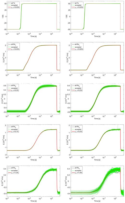
Full periods for transmitter Tx and receivers Rx1–Rx4 (top to bottom) stationary at WP 5 (left-hand panel) and during roll on between WPs 4 and 5 (right-hand panel). Green full periods (about 80 for the WP and 50 for the roll-on data) are selected for stacking (red: stacked full period with mean μ and relative standard deviation σ from the mean), while others are rejected due to erratic noise (grey).
The mean step-on response and the standard deviation of the mean are derived from stacking of the accepted preprocessed data. The stacked data show only a small amount of high-frequency electronic noise. The electrode-drift effect, however, cannot be eliminated completely and imprints systematic errors onto the step-on response.
The 2-D regularized inversion scheme MARE2DEM (Key 2016) treats CSEM data in frequency domain. To transform the selected full periods from time to frequency domain, a fast Fourier transform is applied to each full period. We then calculate the quadratic coherence as a measure of the correlation between the transmitter and receiver signal in frequency domain. The complete procedure is outlined in Appendix A. Frequencies are sampled sparsely for the 2-D analysis as Key (2009) has shown that an increased number of frequencies does not necessarily improve the inversion but increases the computational time. Data points for real and imaginary parts are now chosen, first, logarithmically spaced from 0.5 Hz up to a maximum frequency of 400 Hz, and second, according to their data error, coherence and amplitude. Higher frequencies are generally accepted if the coherence is above 80 per cent. Fig. 8 shows the coherence, real, and imaginary parts, the data error and the chosen data points according to the first criterion (red), as well as the chosen data points for the inversion according to the first and second criterion (green). Due to practical reasons (faster convergence), however, only frequencies smaller 80 Hz have been used for the final inversion after tests have shown that the results do not change when excluding higher frequencies.
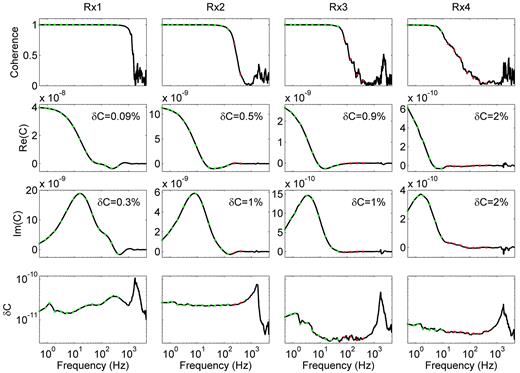
Coherence, real and imaginary parts, and the data error for one roll-on data set. The data points are chosen logarithmically spaced (red) to a maximum frequency of 400 Hz, but are discarded if the data point amplitudes are close to zero, the coherence drops considerably, or the data error increases strongly. The data points that pass these criteria are indicated in green.
3.2 Inversion method and results
Controlled source electromagnetic data contain information about bulk resistivities in the subsurface volume. Typical for diffusion methods, data interpretation for a heterogeneous subsurface resistivity model is non-unique (several subseafloor resistivity models may result in a similar data response). Interpretation requires sophisticated inversion techniques or additional structural constraints to estimate model parameters. Model parameters are often dependent on each other and might only be resolved in combination (e.g. the product of resistivity and layer thickness; Edwards 1997). A widely applied technique is Occam’s inversion (Constable et al.1987) which parametrizes the model using a large number of interfaces/elements at fixed depths such that volume sizes are below the resolution of the data. Occam’s inversion addresses EM diffusion data by smoothest-model regularization (usually represented by an L2 norm which discriminates strongly against abrupt changes) and avoids overfitting the data. The 2-D implementation of Occam’s inversion in MARE2DEM introduces a regularization term using distance-weighted first differences between neighbouring parameters in vertical and horizontal directions (Key 2016).
We did not introduce a dependency on the starting model, and started each inversion with a 1 Ωm half-space model. The model contains three layers with fixed resistivity, one air (1012 Ωm) and two seawater layers (0.2315 and 0.2314 Ωm). The model parameter grid was created including seismic constraints that have been identified by Gehrmann et al. (2015) as common boundaries related to geological structure (shown in Appendix B). The roughness penalty was reduced by 90 per cent for the Holocene base and the unconformity in the Pleistocene sediments, the upper reflector in Fig. 2, to allow for resistivity contrasts at these common boundaries. Stacking errors have shown to be partly smaller than 0.1 per cent for frequencies below 5 Hz and initial inversions did not converge. This can be explained by systematic data errors (e.g. from electrode drift, time synchronizsation, geometry, water resistivity and water depth variations due to tides) being larger for the present data set than stacking errors as previous data residual analysis have shown as well (Gehrmann et al.2015). Therefore, a first inversion with 5 per cent error was performed here. Resulting data residual errors were autocorrelated and converted into a new set of standard deviations following Gehrmann et al. (2015). These standard deviations are about a magnitude larger than the standard deviations derived from stacking, large enough to encompass systematic errors. A second inversion with the new standard deviations was performed, achieving a rms (the square root of the mean square of the difference between observed and predicted data points divided by their standard deviation) of one after five iterations and results are shown in Fig. 9. The observed and predicted data as well as standardized residual errors are shown in Fig. 10 for all receivers. The greater majority of the standardized errors for all receivers, real and imaginary part over frequency pass statistical tests for Gaussianity and randomness (an assumption in the inversion algorithm) .
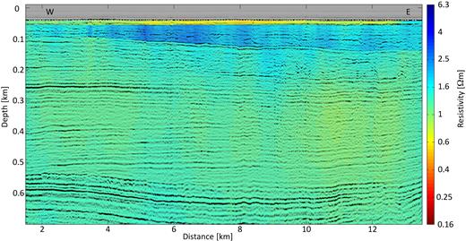
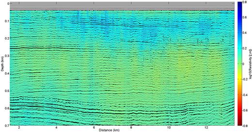
Electrical resistivity from CSEM 2D inversion results on top of seismic depth section AUR03-23a (Fig. 2, location: red line in Fig. 1). Only free parameters (not seawater nor air) are shown. The white half circles are the positions of the source and the triangles the positions of the receivers; tow direction: east to west.
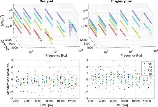
Real and imaginary part of the Earth response (observed data: crosses and error bars; predicted data: circles) and standardized residual errors over transmitter-receiver common mid point (CMP) position along the profile for the four receivers (repeating colour pattern) for every second frequency in Hz. Only every fifth transmitter point is shown for visibility.
The resistivity structure of the 2-D inversion results are similar to the 1-D stitched inversion results by Gehrmann et al. (2015) and Moghadas et al. (2015): First, a conductive (about 1 Ωm) shallow layer, which is about 10 m thick, likely consists of fine-grained Holocene marine deposits. Second, a more resistive layer (about 3 Ωm), which lower boundary is the dipping shallow seismic reflector upR at 100–130 m depth, presumably consists of Pleistocene glacial deposits. Third, a ∼400-m-thick conductive (about 0.7–1.5 Ωm) layer follows. The boundary between the Pleistocene, Pliocene and Miocene sediments is neither distinctly resolved by the seismic nor the CSEM data. However, this third layer mainly consists of several parallel undisturbed layers of fine-grained Miocene floodplain deposits. The resistivity beyond the Mid-Miocene Unconformity at ∼550–600 m depth increases slightly, but the probabilistic 1-D analysis in Gehrmann et al. (2015) have shown that the uncertainties increase at depth below ∼300 m and 95 per cent credibility intervals include a wide resistivity range of up to 0.5–7 Ωm (shown in Appendix B). We can conclude that the inversion results in frequency domain show similar structure than the 1-D inversion results in time domain, which illustrates that the time and frequency domain approach are compatible.
4 DISCUSSION
In this paper we take advantage of a CSEM and a MCS data set collected along a common profile with the aim to resolve the upper sedimentary structure in the shallow North Sea. Instead of processing and modelling each data set purely on its own, we focus on a combined interpretation towards a joint model. There are various benefits in combining both methods, but there are also principle limitations by imaging different physical parameter that do not always have to correlate.
Both methods have a complementary character: Electromagnetic induction is a diffusion process that responds to the electrical resistivity distribution in a volume. The CSEM method is less powerful in resolving exact boundary locations, but sensitive to changes in layer thicknesses (e.g. resistivity-thickness product), porosity or pore fluids. Therefore, CSEM allows deriving volume estimates of hydrocarbon deposits (e.g. shallow gas). In contrast, reflection seismics uses the propagation of elastic waves that provides a boundary response from seismic reflectors. Without reflectors in the subsurface, seismic energy will not return to the source. Receivers measure the seismic waves travelling along a ray path from the source via reflectors to the receiver location. The physical parameter responsible for reflections of seismic waves is an impedance contrast, thus seismic velocity and density changes, marking a layer boundary. The near-vertical seismic method is less powerful in deriving changes in physical properties within a layer (e.g. shallow gas layer), but is powerful in resolving impedance contrasts across layers (e.g. bottom simulating reflector). Therefore, reflection seismics allows imaging structural changes with high resolution even at depth. To summarize, both methods are complementary in the sense that EM images layer volumes while seismics images layer boundaries.
According to the different physical parameter electrical resistivity or seismic impedance, an electromagnetic anomaly does not necessarily have to coincide with a seismic reflector. Therefore, a common model might include an electromagnetic layer that is not imaged by seismic data and vice versa. For example, in case of:
A change of solely pore fluid at constant porosity such as a change from salt water to fresh water, we receive a significant resistivity anomaly but no seismic response at all.
A change of rock density such as a thin layer of gravel within unconsolidated sands, we obtain a prominent seismic reflector but differences in porosity in a thin layer are not sufficient for a pronounced resistivity anomaly due to the too small volume.
Presence of shallow gas even with low saturation of a few per cent we receive a seismic amplitude anomaly with reverse phase due to the significant impedance contrast towards lower seismic velocities—but we do not see a resistivity anomaly as long as saturation and gas volume is low. However, if we have a high gas saturation in the pore volume replacing the conductive pore fluid, we do receive a large resistivity anomaly allowing to estimate the gas volume although the seismic inverse amplitude anomaly does not change significantly.
The combination of CSEM and the seismic reflection method helped us interpreting the presented data especially with regard to the following aspects:
We imported structural constraints from the seismic reflection model in the electromagnetic model. The model cells defined for the 2-D EM inversion code MARE2DEM are stretched out between the imaged seismic reflectors favouring (with decreased regularization penalty) but not forcing the electromagnetic response to accept these boundaries. Structural boundaries from CSEM data alone as shown in the previously published 1-D-inversion models [Bayesian approach by Gehrmann et al. (2015), and the non-linear approach with lateral constrains by Moghadas et al. (2015)] are laterally variable, but it was possible to identify at least two reflectors (Holocene base and Pleistocene unconformity, upR) that also correspond to electric resistivity changes (see Appendix B). Usually the combination of resistivity and layer thickness can be better resolved than each parameters alone. Therefore, including seismic boundaries is a significant improvement for constraining resistivity models.
The interpretation of the layer above reflector upR at 150–200 ms (light brown shaded area in Fig. 5) from EM modelling alone (enhanced resistivities in Fig. 9) might support the interpretation of an increased porosity compared to the layer below (grey-blue shaded area in Fig. 5). However, the seismic model does not support this explanation; increasing seismic velocities below the reflector favour instead a constant increase of sediment compaction and porosity reduction with depth. Therefore, the interpretation of fresh water lenses enhancing the resistivity of the pore fluid is a more likely interpretation in agreement with the seismic data, which cannot distinguish between fresh or salt water pore fluid. Thus, the combination of CSEM and seismic data analysis lead to the interpretation of a possible fresh water lens within the glacial deposits, which is a phenomenon known along the German North Sea coast (Kirsch et al.2006).
The interpretation of the lower reflector loR amplitude anomaly at 300 ms in Fig. 2 with inverse phase and AVO analysis (class III) indicates the presence of gas. Unfortunately, the CSEM profile does not cover the entire anomaly. At least no indication of a resistivity anomaly is visible. The seismic method is not able to discriminate between low and high percentages of gas saturations (Domenico 1976; Ostrander 1984). Because of the small scale of the structure and absence of seismic indicators for fluid pathways (e.g. seismic chimneys), however, we predict only small amounts of gas. Shallow gas occurrences in the North Sea with significant amounts usually show several layers of high reflectivity with chimney or fault structures acting as fluid conduits below (Müller et al.2018).
We demonstrated that the combination of CSEM and seismic data analysis for shallow structures in the North Sea is beneficial and helps to cancel out ambiguities of interpretation. Therefore, we recommend combined surveys with both methods especially over shallow gas deposits. Seismic data will image the structural boundaries, and CSEM data might allow discriminating between significant gas volumes or negligible ones, and between fresh water or saline water lenses. A large number of seismic amplitude anomalies with inverse phase have been mapped in the North Sea. AVO analysis is an important tool to indicate possible gas reservoirs, but volume estimates from seismics alone are difficult and drilling is expensive. CSEM data are only sensitive to large reservoirs with significant gas content above ∼5 per cent. The method has been also tested for monitoring during gas production (Orange et al.2009; Andréis & MacGregor 2011). However, CSEM resolution is decreasing with depth (larger source power and transmitter-receiver offsets will help), but ambiguity can be reduced by including seismic boundaries if they are likely to represent a boundary for both physical properties, seismic impedance and electrical resistivity.
5 CONCLUSIONS
In this study, the combined analysis of CSEM and reflection seismic data enables a more profound geological interpretation of the subsurface. Amplitude Variation with Offset (AVO) analysis of observed data and modelling studies of realistic background trends have shown that the hydrophone array required the calibration of each channel individually to recover amplitudes properly. Two target reflectors were then analysed and classified in class I (water-bearing) and class III (gas-bearing) sediments. Analysis of the CSEM data show little sensitivity to the layer of gas-bearing sediments, which indicates that it is too thin to be resolved or/and the amount of free gas is negligible. The velocity and resistivity increase in the Pleistocene sediments cannot be explained with an increased density as discussed in Gehrmann et al. (2015). Instead, the hypothesis of fresh water within the Pleistocene sediments would support both observations. The resistivity reduces below the Pleistocene unconformity to a minimum for Tortonium deposits. The detailed seismic velocity analysis, that is pre-stack depth migration and reflection tomography, however, results in a general velocity increase with depth that can be explained by sediment compaction with burial and weight of the ice load during the Pleistocene. Both observations support an increasing amount of clay minerals in the Tortonium deposits as indicated by logging data at a drill hole (Thöle et al.2014).
For the first time, we successfully analysed ocean-bottom towed CSEM data acquired while the instrument was moving. Furthermore, we demonstrated that the time and frequency domain analysis of CSEM data are equivalent.
ACKNOWLEDGEMENTS
The authors would like to thank the crew and scientific party of Meteor cruise M88 Leg 2 for acquiring the presented CSEM data sets. Nigel Edwards (retired from University of Toronto) is thanked for supplying parts of the CSEM equipment for the cruise. The project Geo-scientific Potential of the German North Sea (GPDN) was a joint project between the BGR, LBEG and BSH, and was funded by the Federal Ministry of Economics and Technology, the Ministry of Economics, Labour and Traffic of Niedersachsen, and the Federal Ministry of Transport, Building and Urban Development. We thank the GPDN team at the BGR for discussing the geological interpretation, especially Rüdiger Lutz and Lutz Reinhardt. This work was financially supported by funds from RWE DEA AG and EON gas storage. We thank the editor Ute Weckmann and two anonymous reviewers for their efforts which helped improving the manuscript. Last but not least we would like to thank Kerry Key and David Myer for making MARE2DEM and several MATLAB routines available free of charge and well documented.
REFERENCES
APPENDIX A: FREQUENCY DOMAIN TRANSFORMATION
APPENDIX B: SENSITIVITY ANALYSIS OF THE 2D CSEM RESULTS
A section of the inversion results (shown in Fig. 9) is presented in Fig. B1. The inversion grid is made up of triangles with increasing side length from <10 m close to the seafloor to several 100 m at greater depth, with about 22 500 free parameters. A finite source dipole of 100 m length has been implemented for all inversions.
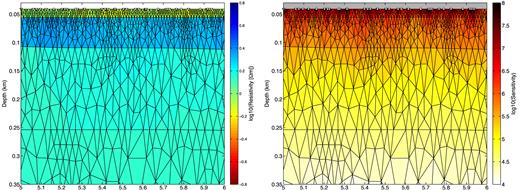
Left-hand panel: final resistivity model for km 5 to 6 with inversion grid overlay. Right-hand panel: cumulative data sensitivity over all frequencies with inversion grid overlay. Circles are source positions while triangles refer to receiver positions.
The cumulative data sensitivity over all frequencies (also shown in Fig. B1) is calculated for small changes around the final model m with |$\sum _{i = 1}^{N}\Delta d_{i}/\Delta m_{j}$| for the ith data point di and the final model’s jth cell. It can be observed that the cumulative sensitivity reduces rapidly with depth and is highest underneath the source and receivers. It is not possible to use the cumulative sensitivity as a quantitative measure for the model uncertainty. To illustrate uncertainties a vertical profile of the resistivity from the model inferred with MARE2DEM (Fig. 9) is shown in Fig. B2 on top of the marginal probability density as a function of depth (as presented in Gehrmann et al.2015) for km 7 along the profile. The probabilistic 1-D approach did not use any constraints, but two resistivity boundaries could be identified from the CSEM data alone. They likely correspond to the base of the Holocene and the upper reflector in the Pleistocene sediments as interpreted from reflection seismic data (Fig. 5).
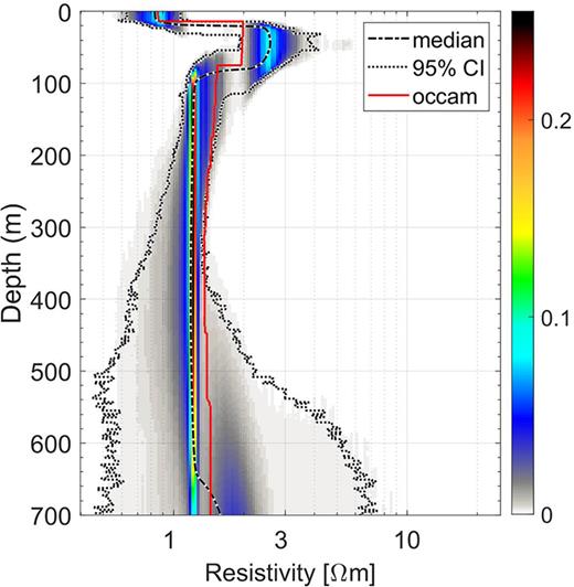
Marginal probability density of resistivity as a function of depth for km 7 along the profile. The median (black dashed line) refers to the posterior median profile and credibility intervals (CI, black dotted lines) contain 95 per cent of all model samples evaluated at each depth interval. Vertical profile from 2-D regularized inversion result (Fig. 9) at km 7 is shown as a red line (occam).
APPENDIX C: INVERSION RESULTS WITHOUT SEISMIC CONSTRAINTS
The electrical resistivity model without seismic constraints is shown in Fig. C1. The inversion converged after three iterations. The model consists of four layers with different resistivities similar to Fig. 9. The resistive layer below the conductive top layer is less resistive but thicker. This ambiguity arises from CSEM data being sensitive to the resistivity-thickness product more than to the individual parameters themselves (e.g. Flósadottir & Constable 1996). Another constraint in the inversion is that the roughness penalty is three times larger in horizontal direction than vertical direction, assuming that resistivity changes in the vertical direction are more likely than in the horizontal, but tests have shown that the inversion results vary only little when changing this factor. We have also tested if the resistivity models could be anisotropic as anisotropy in horizontal against vertical direction can be quite large in sedimentary rocks (Myer et al.2015). Here, however, anisotropic inversions yield the same results as isotropic inversions with little variation of horizontal to vertical resistivity. This observation supports that the sediments are mostly unconsolidated and non-directional (especially the unsorted glacial deposits).
Depth-migrated reflection seismic data of AUR03-23a on top of resistivity model for an unconstrained inversion.
