


Summary
Several researchers have studied the source parameters of the 2005 Fukuoka (northwestern Kyushu Island, Japan) earthquake (Mw 6.6) using teleseismic, strong motion and geodetic data. However, in all previous studies, errors of the estimated fault solutions have been neglected, making it impossible to assess the reliability of the reported solutions. We use Bayesian inference to estimate the location, geometry and slip parameters of the fault and their uncertainties using Interferometric Synthetic Aperture Radar and Global Positioning System data. The offshore location of the earthquake makes the fault parameter estimation challenging, with geodetic data coverage mostly to the southeast of the earthquake. To constrain the fault parameters, we use a priori constraints on the magnitude of the earthquake and the location of the fault with respect to the aftershock distribution and find that the estimated fault slip ranges from 1.5 to 2.5 m with decreasing probability. The marginal distributions of the source parameters show that the location of the western end of the fault is poorly constrained by the data whereas that of the eastern end, located closer to the shore, is better resolved. We propagate the uncertainties of the fault model and calculate the variability of Coulomb failure stress changes for the nearby Kego fault, located directly below Fukuoka city, showing that the main shock increased stress on the fault and brought it closer to failure.
1 INTRODUCTION
Earthquakes occur when shear stresses on a fault overcome clamping of normal stresses and friction. The Coulomb failure criterion (Harris 1998; King et al.1994; Stein et al.1992) is used to characterize the stress conditions at which failure can occur. An earthquake modifies the stresses in the surrounding rocks and may thus either delay the next earthquake on a nearby fault or hasten it according to this failure criterion. A nearby mapped fault is considered moved closer to failure if changes in Coulomb failure stress (ΔCFS) due to an earthquake are positive and is further from failure if ΔCFS is negative (e.g. Deng & Sykes 1997; Hincapie et al.2005; Hodgkinson et al.1996; Lin & Stein 2004; Nalbant et al.1998; Parsons et al.2000, 2008; Stein et al.1994, 1997).
Many past studies focused on stress interactions between earthquakes. Deng & Sykes (1997) found that 95 per cent of magnitude 6.0 and greater earthquakes with strike-slip and dip-slip mechanisms in southern California occurred in areas of increased ΔCFS. Stein et al. (1997) inferred that nine out of 10 large earthquakes along the North Anatolian Fault between 1939 and 1992 occurred where ΔCFS was increased by the previous earthquake. Parsons et al. (2000) showed that the 1999 Izmit earthquake (Mw7.6) occurred in an area of increased stress, which in turn increased ΔCFS on a fault in Düzce that ruptured three months later. Nalbant et al. (1998) studied the stress interaction between faults in the backarc extensional region of the northern Aegean Sea and between segments of the North Anatolian Fault in the Sea of Marmara where there had been large earthquakes in the past. They found that 23 of the 29 events (strike-slip, normal and oblique fault mechanisms) occurred in areas of increased Coulomb stress due to preceding earthquakes. Similarly, Doser & Robinson (2002) found that six of the seven events with magnitude between 5.9 and 7 in southern Marlborough region, east of the Alpine fault in New Zealand, occurred where the ΔCFS was increased by the preceding earthquake by 10 kPa or more.
Most studies of ΔCFS have ignored uncertainties in the calculated ΔCFS although such uncertainties can be quite significant and can vary at different locations around the source fault (Woessner et al.2012). These uncertainties can be calculated by propagating uncertainties in the fault model (Hainzl et al.2009; Lohman & Barnhart 2010; Woessner et al.2012) and by including uncertainties in the geometry of the receiver fault (Steacy et al.2005). Estimating a fault model with unknown geometry from geodetic data is a non-linear problem, in which uncertainties of estimated parameters arise from uncertainties in the data and the earth model.
Uncertainties in fault model parameters have been quantified in the past by obtaining an ensemble of fault models describing the data (e.g. Cervelli et al.2001; Duputel et al.2014; Fukuda & Johnson 2008; Funning et al.2005; Monelli et al.2009; Sudhaus & Jónsson 2009, 2011; Sun et al.2011; Xu et al.2015). Some authors have used Bayesian estimation of the fault-slip model parameters to obtain their posterior distributions (e.g. Duputel et al.2014; Monelli et al.2009; Fukuda & Johnson 2008; Sun et al.2011; Xu et al.2015). However, they used only geodetic and/or seismic data to constrain the fault parameters, even though the Bayesian method also allows auxiliary physical information about the fault to be used when constraining the fault-slip model. Although some regularization constraints (like slip smoothness) have previously been used as a priori information about fault-slip patches (Fukuda & Johnson 2008), physical constraints on the fault geometry (such as strike and dip), for example, from locations and focal mechanisms of aftershocks, or from the moment magnitude of the earthquake, have seldom been used in Bayesian estimation. Such physical constraints can be useful with limited data that poorly constrain the fault model (e.g. Xu et al.2015). In this paper, we show how locations of aftershocks and the magnitude of the main shock can be used as a priori information in Bayesian fault model estimation.
We use the 2005 |$M_{\rm {\rm w}}\,6.6$| Fukuoka earthquake as a case study. This earthquake occurred about 20 km offshore and northwest of Fukuoka city (northern Kyushu Island, Japan), which had a population of 1.4 million in 2005 (Fig. 1). It ruptured a previously unknown fault with a left-lateral strike-slip. This fault is now considered to be an extension of the Kego fault (Shimizu et al.2007), which was mapped by Karakida et al. (1994), has a similar NW–SE trend, and lies directly under Fukuoka city. A possible future earthquake of similar magnitude on the Kego fault would be devastating to the city and might threaten critical facilities, such as the Genkai nuclear power plant, which is only about 50 km away from the Kego fault.
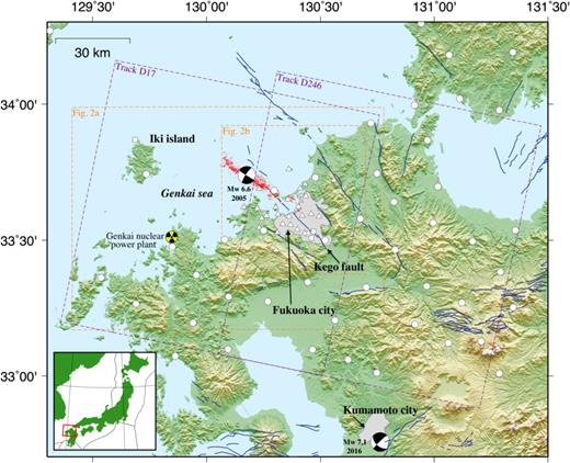
Shaded-relief topographic map of northwestern Kyushu (inset shows the location in Japan). Mapped active faults are shown in blue (Active fault database of Japan, AIST) and aftershocks as red dots (Uehira et al., 2006). Locations of GEONET continuous GPS stations (white circles), other continuous stations (white squares), as well as campaign GPS stations (white triangles) are also shown. Purple dashed rectangles mark areas covered by the descending radar scenes and orange rectangles the coverage of Fig. 2.
The Fukuoka earthquake was studied shortly after it took place by several researchers, for example, by using teleseismic, strong motion and geodetic data (Asano & Iwata 2006; Horikawa 2006; Kobayashi et al.2006; Nishimura et al.2006; Ozawa et al.2006; Sekiguchi et al.2006; Suzuki & Iwata 2006; Takenaka et al.2006). However, none of these authors reported uncertainties in their fault solutions, making it difficult to assess differences between solutions and the reliability of calculated ΔCFS on and near the Kego fault. In this study, we use both Global Positioning System (GPS) and Interferometric Synthetic Aperture Radar (InSAR) data to constrain the offshore fault location and geometry. We also develop an approach to include the magnitude of the main shock and the locations of the aftershocks as a priori information in constraining the model parameters. To understand the stress interaction between the fault that ruptured and the Kego fault, we calculate the ΔCFS along the Kego fault and assess the reliability of ΔCFS by propagating the fault model uncertainties in the calculation.
2 STUDY AREA
The Mw6.6 Fukuoka earthquake occurred at 10:53 a.m. on 2005 March 20 (JST) beneath the Genkai Sea, northwest of Shika Island (or Shikanoshima in Fig. 2), which is located just off the northwestern coast of Kyushu Island in Japan. One death was confirmed and around 1000 people were injured in the earthquake. It also caused severe damage to buildings on Genkai Island (Fig. 2) and the total economic loss was estimated to be about 150 million US dollars. The tectonics in northern Kyushu is less active than in most other parts of Japan, the last large earthquake in the region being the 1700 Mw7 Tsushima earthquake (Matsumoto et al.2006). The last destructive earthquake in northern Kyushu was the 1898 MJMA6 Itoshima earthquake (Shimizu et al.2007). The tectonics around the northern coast of Kyushu is characterized by N–S extension with a crustal strain rate of approximately 5e-8 yr−1 during the past 100 yr (Shimizu et al.2007). Most seismicity in Kyushu is related to the subduction of the Philippine Sea plate at depth. An Mw7.1 earthquake ruptured beneath Kumamoto city in central Kyushu in 2016 April, causing 35 deaths and around 2000 injuries. This earthquake followed magnitude Mw6.2 and 6.0 foreshocks that occurred in the same region and caused nine fatalities. Central Kyushu also experienced two earthquakes of magnitudes 5.8 and 6.1 in 1975 January and April, respectively. These earlier earthquakes occurred 40–60 km northwest of the later 2016 event and caused injuries, but no known fatalities.
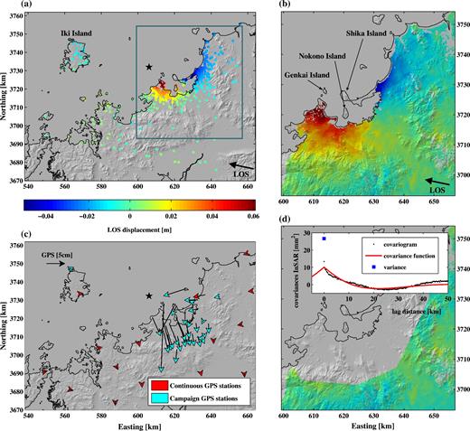
Observed coseismic displacements caused by the Fukuoka earthquake. (a) Results of stable point target analysis of descending ENVISAT data from track 17 (in UTM coordinates, zone 52S), showing observed ground displacements into the Line-Of-Sight (LOS) towards the satellite as positive. Blue rectangle shows the coverage of parts (b) and (d). (b) Descending ENVISAT interferogram from track 246. (c) Horizontal GPS displacements obtained from continuous and campaign GPS stations. The black star in (a) and (c) indicates the epicentre of the earthquake. (d) Variance, sample covariogram and fitted covariance function (figure inset) of the noise of the undeformed region (shown) of data from track 246.
The Fukuoka earthquake occurred on a previously undocumented NW–SE fault with a predominantly left-lateral strike-slip. Uehira et al. (2006) deployed 11 ocean-bottom seismometers and 24 temporary on land stations around the aftershock area to locate the aftershock activity and provide information on the location of the source fault of the main shock (Fig. 1). These aftershock locations suggest that an approximately 25 km long NW–SE striking fault ruptured during the main shock, which was nearly vertical at depths of 2–16 km (Shimizu et al.2007). No surface ruptures on the seafloor were found during a sonic prospecting survey carried out by the Japan Coast Guard after the earthquake (Sekiguchi et al.2006; Takenaka et al.2006). From focal mechanisms of 1333 aftershocks and using a damped regional-scale stress inversion technique (Hardebeck & Michael 2006), the maximum principal compressive stress (σ1) and the minimum principal stress (σ3) were estimated to be directed WSW–ENE and NNW–SSE, respectively (Matsumoto et al.2012).
As noted, several studies focused on estimating the fault parameters of the earthquake using teleseismic, strong motion and geodetic data (Table 1). Nishimura et al. (2006) used GPS and InSAR data to estimate the fault-slip distribution, however only one InSAR interferogram (from descending track 17 of the ENVISAT satellite) was used in their analysis. This interferogram has limited data in both the near-field and the far-field due to the offshore location of the earthquake and decorrelation. Their slip model has a seismic moment of 8.7 × 10¹⁸ N·m, strike of N118°E, dip of 79° (dipping to the northeast) and rake of 18°. Ozawa et al. (2006) also used GPS and InSAR data to estimate the slip distribution on a fault with a fault dip of 90° and a strike of 122°. They found maximum left-lateral strike-slip of 2.4 m, with the slip exceeding 1 m shallower than 10 km at the centre of the fault and shallower than 4 km close to the coast.
Information about fault solutions for the 2005 Mw 6.6 Fukuoka earthquake estimated by different agencies/authors. Dips and strikes are according to the parametrization in our study. Faults with dip less and more than 90° are dipping towards NE and SW, respectively. * indicates finite-fault solutions where the seismic moment is computed by summing up the slip amplitudes in each patch. |$^\#$| indicates the solutions where only the deviatoric component of the moment tensor is constrained and their scalar moment is computed from the dominant eigenvalues of the moment tensor. |$^{\#\#}$| indicates the moment tensor solution where the scalar moment is computed from the L2 norm of the eigenvalues of the moment tensor.
| Solution | Data used | Seismic moment [N·m] | Centroid location | Strike | Dip (° ) | Rake (° ) |
|---|---|---|---|---|---|---|
| (Moment magnitude) | (°E, °N, km) | (N °E) | ||||
| GCMT | Teleseismic | 9.02 × 10¹⁸ (6.602)|$^\#$| | 130.15, 33.72, 12 | 122 | 88 | −14 |
| NEIC | Teleseismic | 1.052 × 10¹⁹ (6.639)|$^{\#\#}$| | 130.131, 33.807, 10 | 125 | 117 | −16 |
| NIED F-net | Local broadband | 7.8 × 10¹⁸ (6.565)|$^\#$| | 130.17, 33.74, 11 | 122 | 93 | −11 |
| Ito et al. (2006) | Strong motion, | 8.4 × 10¹⁸ (6.586)|$^\#$| | 130.18, 33.74, 10 | 123 | 94 | −4.3 |
| local broadband | ||||||
| Nishimura et al. (2006) | InSAR, GPS | 8.7 × 10¹⁸ (6.596)* | 130.297, 33.683, 7.4 | 118 | 101 | −18 |
| Asano & Iwata (2006) | Strong motion | 1.15 × 10¹⁹ (6.677)* | 130.1918, 33.7363, 8.14 | 122 | 93 | |
| Takenaka et al. (2006) | Strong motion | 124 | 87 | −11 | ||
| Horikawa (2006) | Strong motion | 5.7 × 10¹⁸ (6.474)* | 130.2011, 33.7210, 12 | 122 | 91 | 8 |
| Kobayashi et al. (2006) | Strong motion, | 1 × 10¹⁹ (6.637)* | 130.2486, 33.7074, 6 | 123 | 92.3 | −1 |
| 1-Hz GPS | ||||||
| Sekiguchi et al. (2006) | Strong motion | 1.16 × 10¹⁹ (6.68)* | 130.2482, 33.6985, 4 | 126 | 93 | |
| Ozawa et al. (2006) | InSAR, GPS | 130.2016, 33.7264, 5 | 122 | 90 | ||
| |$130.175_{-0.0102}^{+0.007}$|, | ||||||
| Our solution | InSAR, GPS | |$8^{+0.6}_{-0.65}\times 10^{18}$| (|$6.568^{+0.021}_{-0.024}$|)* | |$33.7312^{+0.0071}_{-0.0035},$| | |$121.4^{+2}_{-1.95}$| | |$95_{-5.7}^{+2.8}$| | |
| |$8.354_{-0.84}^{+1.23}$| |
Asano & Iwata (2006) performed a kinematic waveform inversion using strong motion data to study the fault rupture process. They observed that the rupture mainly propagated to the southeast from the hypocentre. They observed two slip asperities with the smaller slip asperity shallower and the larger slip asperity deeper than the hypocentre. They estimated the seismic moment to be 1.15 × 10¹⁹ N·m. Horikawa (2006) also used strong motion data to study the rupture process and also found two slip asperities with the shallower asperity smaller than the deeper asperity. However, they found that the rupture propagated bilaterally with a lower seismic moment (5.7 × 10¹⁸ N·m). Kobayashi et al. (2006) used both strong motion and 1-Hz GPS data and estimated the seismic moment to be 1 × 10¹⁹ N·m, with the rupture propagating SE from the hypocentre with only one asperity shallower than the hypocentre.
In yet another study using strong motion data, Sekiguchi et al. (2006) estimated the seismic moment release to be 1.16 × 10¹⁹ N·m and the rupture velocity to be 2.1 km s−1. Their estimated slip distribution shows a single asperity that is about 6 km × 8 km in size. Their solution indicates that the rupture propagated mainly to the southeast and that it started with a high slip rate at the hypocentre, continuing at a low slip rate for a few seconds, and then returning to a high slip rate in the southeast and shallower than the hypocentre. Takenaka et al. (2006) used strong motion data to estimate the geometry of the fault plane and they found a fault strike of N124°E and a fault dip angle of 87° (dipping to the NE). They then estimated that the fault ruptured in two asperities with the main rupture onset location 5 km southeast from the hypocentre. They estimated a slow rupture velocity of 1.4 km s−1, which is 40 per cent of the shear wave velocity.
Most of these kinematic rupture models were estimated using a fault geometry obtained from poorly constrained aftershocks and focal mechanisms that were reported without any uncertainties. In addition, none of the earlier studies reported uncertainties in their fault model solutions. Uncertainties in the source fault solutions directly influence the reliability of ΔCFS calculations (Lohman & Barnhart 2010; Woessner et al.2012). Here, we consider the influence of the source model errors on ΔCFS calculations around the Fukuoka earthquake and in particular along the Kego fault.
3 DATA
We used both GPS and InSAR data to estimate the fault geometry and average slip of the Fukuoka earthquake (Fig. 2). The radar data were acquired from two parallel descending tracks by the ENVISAT satellite (tracks 17 and 246). We used the Gamma processing software (Werner et al.2000) to process the raw SAR data, process the interferograms, and remove the topography-related phase using the Shuttle Radar Topography Mission (Farr et al.2007) 3-arcsec digital elevation model. We generated a single good-quality interferogram with small temporal and spatial baseline from descending track 246. The signal-to-noise ratio of the interferogram was enhanced by multilooking and adaptive spectral filtering (Goldstein & Werner 1998). We then unwrapped the interferogram using a minimum cost-flow algorithm (Chen & Zebker 2002) and removed a phase ramp by considering the phase in the far-field to be close to zero. It was not possible to generate good-quality interferograms from descending track 17 due to temporal and baseline decorrelation (Zebker & Villasenor 1992) and atmospheric noise. Instead, we used all the available SAR scenes from this track (Fig. S1, Supporting Information), from both before and after the earthquake (21 SAR scenes), to detect stable point targets based on phase coherence. For each point target, we generated displacement time-series from the unwrapped interferograms (formed from the 21 SAR scenes, see Fig. S1, Supporting Information) and fitted a step function to estimate the coseismic displacement. Before the modeling, we subsampled all the InSAR data using the quadtree algorithm (Jónsson et al.2002).
InSAR data from track 246 contain data from only the east side of the fault and mostly from the mainland (Fig. 2b), while data from Shika, Genkai and Nokono Islands, which are within 10 km of the fault are lost due to decorrelation. This data set shows a maximum line-of-sight (LOS) uplift of ∼6 cm and maximum LOS subsidence of ∼5 cm (Fig. 2b). The stable point-target data from track 17 have better coverage, extending to Iki Island, located to the west of the earthquake, and also to Shika, Genkai and Nokono Islands. This data set shows maximum LOS uplift of ∼8 cm and maximum LOS subsidence of ∼4 cm (Fig. 2a).
We also used GPS data measured at 56 continuous GPS stations and 26 campaign GPS survey sites (Fig. 1). All but four of the continuous GPS stations are from GEONET (GNSS Earth Observation Network System) maintained by GSI (Geospatial Information Authority of Japan). The remaining continuous GPS stations are maintained by GSI for public surveying and one by the Hydrographic and Oceanographic Department of the Japan Coast Guard. The coseismic displacements were derived from the difference in the averages of daily solutions between 2005 March 10–19 and 21–30. Maximum horizontal displacement of 20 cm and vertical displacement of 4 cm were observed at the Shika Island station (Fig. 2c).
The campaign GPS measurements at the 26 sites were carried out by GSI on 2005 March 27–31. The pre-seismic measurements were mostly from 1994. The maximum coseismic horizontal displacement of 38 cm was observed on Genkai Island (Fig. 2c). These measurements include contributions from interseismic displacements between 1994 and 2005 as well as errors related to the centring of the GPS antennae. The accuracy of the vertical campaign GPS displacements is low compared to that of the horizontal displacements. In general, the uncertainties of the campaign GPS measurements are much larger than those of the continuous GPS measurements (Nishimura et al.2006). The uncertainties are accommodated accordingly in the data covariance matrix used in the estimation.
4 METHODOLOGY
We used Bayesian estimation to determine the fault model parameters of the Fukuoka earthquake. In the Bayesian approach, we estimate the multidimensional posterior probability distribution function (PDF) defined on the model space using an iterative stochastic Markov Chain Monte Carlo (MCMC) method. This posterior PDF incorporates specified prior information about the model space, and the physical law relating the model parameters with the data (linearly or non-linearly). The model parameter uncertainties are then analysed from the 1-D and 2-D posterior marginal PDFs. Here, we begin by describing the parametrization of the fault-slip model and then we present the formulations of the prior PDF, the likelihood function and the posterior PDF.
4.1 Fault model parametrization
The model parameter vector, m in the M-dimensional model space |$\mathbb {M}$|, in our problem relates non-linearly to the data vector, d in the N-dimensional data space |$\mathbb {D}$|: d = G(m) + ε1, where G(m) are the predicted data with ε1 errors. Here, the unit of d, G(m) and ε1 is metres. We used a rectangular planar fault with a uniform left-lateral strike-slip placed within a homogeneous and isotropic elastic half-space to represent our fault model (Okada 1985), which can be parametrized by eight parameters. The seven geometrical parameters are the easting and westing coordinates of the two endpoints of the fault (top edge), the fault depth (from the top edge), width and dip. The eighth parameter is the amount of left-lateral strike-slip on the fault surface. We chose to estimate the endpoint locations of the fault, instead of using one centre coordinate along with the fault's length and strike, as the data can constrain the near-shore east end of the fault much better than its west end, which is located further offshore (Fig. 1). The dip-slip parameter was set to zero for simplicity and because the Fukuoka earthquake was predominantly a left-lateral strike-slip event.
4.2 Bayesian inference
4.2.1 Likelihood function
4.2.2 Prior probability distribution
The prior probability distribution ρM(m) (or simply prior) can be some physical knowledge we have about the model parameters, for example, from some independent sources. Due to lack of a priori physical knowledge and to reduce complexity, the prior has usually been chosen as an uninformative prior distribution (Fukuda & Johnson 2008, 2010; Xu et al.2015). However, informative priors can be very useful as they reduce the solution space of the model parameters and can exclude unphysical model solutions. We use information about the moment magnitude of the main shock and locations of the aftershocks as informative priors to constrain the fault parameters of the Fukuoka earthquake. For ease in the sections later, we divide the fault parameters in m into two groups, parameters m1 that control the fault slip and dimensions of the fault, and parameters m2 that control the location of the fault (m = m1 ∪ m2).
- Moment magnitude: Due to the offshore location of the main shock, the geodetic data do not constrain the dimensions of the fault well, leading to highly variable model solutions and large differences in the moment magnitude. By using a moment magnitude prior, we can restrict the fault models to a specified magnitude range and reject models with very high or very low moments. The moment magnitude in both the Global Centroid Moment Tensor (gCMT) catalogue and USGS National Earthquake Information Center (NEIC) catalogue is 6.6. Also, the mean of the moment magnitudes estimated previously using GPS and InSAR data (Nishimura et al.2006; Ozawa et al.2006), using strong motion data (Asano & Iwata 2006; Kobayashi et al.2006; Sekiguchi et al.2006) and using broad-band strong motion data (Suzuki & Iwata 2006) is 6.6 (estimated from Table 1). Hence, the moment magnitude is considered to follow: Mw(m1) + ε2 = 6.6, where the error, ε2, is considered to be Gaussian with zero mean and variance of h12 (a hyperparameter that is estimated a priori and discussed later). The moment magnitude relates non-linearly to the fault model parameters: |$M_w({\bf m}_1)=\frac{2}{3}\log {M_o({\bf m}_1)}-6.03$|, where Mo is the seismic moment in N·m given by Mo(m1) = μ · Lm · Wm · sm, where μ is the material shear modulus (in Pa), Lm and Wm are, respectively, the fault length and width, and sm is the slip. We use a shear modulus of 32 GPa. Here, Mw(m1) and h1 are both dimensionless quantities. The moment magnitude prior PDF, ρ(m1), is considered proportional to |$\rho (M_w({\bf m}_1))=\mathcal {N}(6.6,{h_1}^2)$| and is given as:(5)\begin{equation} \rho ({\bf m}_1) \propto \exp \left[-\frac{1}{2{h_1}^2}\big (M_w({\bf m}_1)-6.6\big )^2\right]. \end{equation}
- Aftershock locations: The geometry and location of the fault plane can be estimated through non-linear optimization using geodetic data (Jónsson et al.2002) or it can be estimated from aftershock locations (Custódio et al.2009). In this study, we use geodetic data to estimate the fault geometry and use aftershock locations as an informative prior. This means that fault models that are not in accordance with the aftershock locations are more likely to be rejected during the MCMC sampling. We use precise locations of the aftershocks from Uehira et al. (2006) to define this informative prior. Considering there are L number of aftershock locations, we define an L-dimensional vector, D(m2), which is comprised of the perpendicular distances between the aftershocks and the fault plane, m2 (Appendix A). Here, D(m2) follows the relation: D(m2) = ε3, where ε3 is the L-dimensional random error. We assume this error to follow a Gaussian distribution with null-vector mean and variance of h22Σl, where Σl is a diagonal matrix that incorporates the errors in the aftershock locations and h22 is a hyperparameter. Here, the unit of D(m2) is m, that of Σl is m2, and h2 is a dimensionless quantity. The aftershock locations prior PDF ρ(m2) is considered proportional to |$\rho (D({\bf m}_2))=\mathcal {N}({\bf 0},{h_2}^2\Sigma _l)$| and is defined as follows:(6)\begin{equation} \rho ({\bf m}_2) \propto \exp \left[-\frac{1}{2{h_2}^2}D({\bf m}_2)^T\Sigma _l^{-1}D({\bf m}_2)\right]. \end{equation}
4.2.3 Posterior probability distribution
4.2.4 Estimation of hyperparameters
In eq. (9), H12 and H22 are the hyperparameters that control the relative weight of the corresponding prior with respect to the data. Using informative priors in the Bayesian framework requires estimation of these hyperparameters. For indirect prior constraints (for e.g. fault slip smoothness constraint in distributed fault-slip estimation), the hyperparameters have been objectively estimated either by using Akaike's Bayesian Information Criterion (ABIC, Akaike 1980; Funning et al.2014; Yabuki & Matsu'ura 1992) or by including them as additional parameters in the Bayesian inference (Fukuda & Johnson 2008, 2010). In the case of direct prior constraints (for e.g. bounds on the model parameter space) that relate either linearly (Hashimoto et al.2009; Jackson 1979; Matsu'ura et al.2007) or non-linearly (Matsu'ura & Hasegawa 1987) to the model parameters, the hyperparameters have been chosen based on the prior information. Here, the direct prior constraints are non-linearly related to the model parameters and the hyperparameters are subjectively chosen based on a priori information about the fault models.
The variance of the Gaussian magnitude prior distribution (in eq. 5), h12 (= 1/H12), is estimated from the moment magnitudes reported in previous fault solutions (Table 1). The standard deviation of the moment magnitudes reported by previous researchers and agencies is estimated to be 0.0634 and this value is allocated as the standard deviation of the prior distribution (h1). The hyperparameter, H12, thus assigned in eq. (9), is 248.78. The hyperparameter H22 (= 1/h22) is estimated from the characteristics of the aftershock locations. The aftershock locations are used to estimate the best-fitting plane and its uncertainties using Bayesian inference (Appendix B). From this best-fitting plane and its uncertainties, the distribution of |$D({\bf m})^T\Sigma ^{-1}_l D({\bf m})$| (in eq. 6 and Fig. B1) is estimated and the standard deviation of this distribution is used as the standard deviation of the aftershock Gaussian prior distribution (h2 in eq. 6). The hyperparameter, H22, thus assigned in eq. 9, is 0.00281.
4.2.5 Sampling algorithm
Suppose x(i) is the initial model sample, g(x) is the target distribution that needs to be sampled and q(x|x(i)) is the proposal distribution used to generate a model sample from the initial model sample.
Generate a model sample x* from the previous candidate model sample x(i) using the proposal distribution x* ∼ q(x|x(i)). We use a multidimensional Gaussian proposal distribution q(x|x(i)) with mean x(i) and standard deviation 1/10th of the range of the corresponding model parameter space.
- Calculate the acceptance probability, φ(x(i), x*), from the relationSince the proposal distribution is symmetric (Gaussian), then q(x*|x(i)) = q(x(i)|x*).(12)\begin{equation} \varphi ({\bf x}^{(i)},{\bf x}^*)= \min \left[1,\frac{g({\bf x}^*)}{g({\bf x}^{(i)})} \frac{q({\bf x}^{(i)}|{\bf x}^*)}{q({\bf x}^*|{\bf x}^{(i)})} \right] \end{equation}
Set the next candidate model sample, x(i + 1) = x*, with probability φ(x(i), x*), otherwise set x(i + 1) = x(i). The model sample x* is always selected to be a candidate sample if g(x*) > g(x(i)), which means that the more probable model samples are always selected. If the move is towards a less probable model sample, the move is sometimes rejected, depending on the relative drop in probability. The larger the relative drop in probability is, the more likely it is that the next model sample is rejected. Thus, the algorithm preferentially samples high probability regions of the model space while occasionally sampling from low probability regions.
Repeat the process from step (ii).
Using this algorithm, we generated 100 000 samples from 10 independent chains, each with a different initial model. The average acceptance rate was ∼ 27 per cent for all the chains. The samples were tested for the convergence diagnostic using the Gelman and Rubin Multiple Sequence Diagnostic test (Gelman & Rubin 1992) by calculating the potential scale reduction factor (PSRF) from the within-chain and between-chain variances (see Supporting Information 3). PSRF close to 1 indicates that the chains converged to a stationary distribution and that the samples drawn represent the posterior distribution. The first 20 per cent of the samples of each chain, corresponding to a burn-in period, were removed and then the sample chains were thinned to 8000 samples to reduce sample correlation (Fig. S2, Supporting Information).
4.2.6 Error statistics
We derived the data error of the continuous GPS displacements from standard deviations of daily coordinate solutions, which yielded a 1–6 mm error in the horizontal displacements and a 4–15 mm error in the vertical displacements. The errors in the campaign GPS data are larger, about 50 and 100 mm for the horizontal and vertical components of the displacements, respectively. The relative weights of the campaign and continuous GPS are 7.5 and 92.5 per cent, respectively.
5 RESULTS
In this section, we present the results of the Bayesian estimation using informative priors. Fig. 4(a) shows the 1-D and 2-D marginal posterior PDFs of the model parameters obtained from the ensemble of models that were sampled. As expected, the data constrain the eastern end of the fault better than they constrain its western end (Fig. 4b). The 95 per cent confidence ellipse for the location of the fault's western end has a length of 9 km, whereas the ellipse for the location of the fault's eastern end is 5 km. This reflects the fact that the data coverage is much better east of the earthquake (see Fig. 2a). The 1-D posterior distribution of the fault length shows high probability at 11–14 km (Fig. 5), which is somewhat shorter than what the aftershocks indicate (Fig. 3) and is influenced by the uniform-slip parametrization of the fault. The endpoint locations of the fault correlate with the amount of left-lateral fault slip such that longer faults have less slip and smaller faults have more slip. The uniform left-lateral strike-slip varies from 1.2 to 3 m.
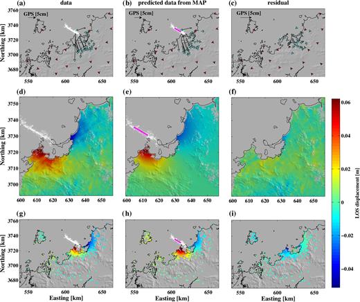
Model prediction and residuals using the maximum a posteriori fault parameters. (a) Data, (b) model prediction, (c) residuals for the GPS horizontal data, (d)–(f) for the track 246 data and (g)–(i) for the track 17 subsampled point-target data. The aftershocks are shown as white dots. The surface projection of the best-fitting source fault (MAP), which is close to vertical, is shown in purple; and the thick line marks the upper edge of the fault.
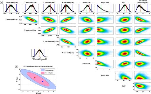
(a) 1-D and 2-D marginal PDF plots of the fault model parameters estimated using both moment magnitude and aftershock location priors. Blue lines in the 1-D marginal PDF plots show the 95 per cent confidence interval, the red line shows the maximum a posteriori (MAP) value and the green dashed line shows the posterior mean value. Hot colours in 2-D marginal PDF plots show high probability regions and cold colours show low probability regions. The pink dot in 2-D marginal PDF plots shows the MAP value. The MAP estimate (pink dots and red lines) is within 0.225-σ of the true MAP. (b) 2-D marginal PDF with means removed for easting and northing of western (blue ellipse) and eastern endpoints (red ellipse) of the fault. The maximum a posteriori (with means removed) solution of western (blue dot) and eastern endpoints (red dot) are overlaid.
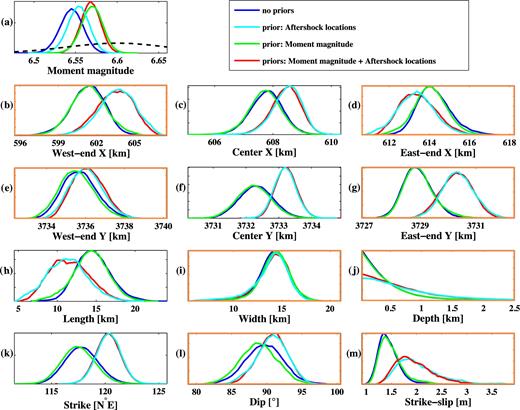
Comparisons of 1-D marginals of the model parameters estimated using no priors (blue), only the aftershock locations prior (cyan), only the magnitude prior (green) and both priors (red). The black dashed line in (a) shows the moment magnitude prior distribution used. The fault model parameters that were sampled for using Bayesian inference are shown in orange boxes and the parameters derived from them are shown in black boxes.
The depth of the fault is shallow and fault models that rupture the seafloor explain the data better. The depth correlates strongly with the fault width with deeper faults having smaller widths. The 1-D posterior distribution for fault width peaks at ∼14 km. The fault is close to vertical with the fault dip ranging from 85° to 95° to the southwest and peaking at ∼90° (vertical fault). The uniform left-lateral slip correlates with most parameters that control the location of the fault. The moment magnitude discerned from the marginal posterior PDF (see Fig. 4) varies from 6.54 to 6.6 with a peak at 6.568, whereas the moment magnitude prior was centred at 6.6 with a standard deviation of 0.0634. The maximum a posteriori (MAP) values of most of the fault parameters (red line in 1-D marginal PDFs in Fig. 4) are similar to the posterior mode values of those parameters. The posterior mean values (green dashed lines in Fig. 4), on the other hand, are somewhat different than the MAP values, especially for the fault width, depth and slip. Fig. 3 shows the different data sets, predicted data from the MAP model and the residuals.
5.1 Effect of informative priors
As discussed above, we used informative a priori constraints on the fault model parameters due to the limited coverage of the geodetic data in our study. Here, we examine the effect that these informative priors have on the estimation. Fig. 5 shows the 1-D marginal posterior distributions of the fault model parameters for four different cases: use of uniform (uninformative) priors, use of a magnitude prior, use of an aftershock locations prior and use of both magnitude and aftershock locations priors.
The peak of the magnitude marginal distribution shifts from 6.546 to 6.568 when the moment magnitude prior is added, but this prior does not much affect other posterior marginals of the fault parameters (Fig. 5). This is due to the fact that the data, though sparse, are capable of estimating the moment magnitude with an uncertainty that is one-tenth of a unit (Fig. 5a) and that a moment magnitude prior with larger standard deviation than the moment magnitude estimate has limited effect in the estimation. Using this prior is more effective when the data errors are high and the estimation is less certain (Xu et al.2015).
In contrast, the marginal distributions of most of the fault-slip model parameters when using the aftershock locations prior are systematically different from the results that do not include that prior. When using the aftershocks prior, the length of the fault is smaller and the uniform left-lateral slip is larger. The distribution for fault strike shows that the aftershock locations prior leads to a tighter constraint on strike, which peaks at ∼120°. The fault parameters that control the fault strike in our parametrization, that is, the easting and northing of the ends of the fault are less variable than without this prior (see Fig. 5). Due to the offshore location of the earthquake and lack of the near-field geodetic data, the constraint on the strike is biased. The aftershock locations thus clearly help to constrain the strike of the fault.
When using both the moment magnitude and aftershock locations priors, most of the resulting fault parameters are similar to the case when only the aftershock locations prior is used. However, the use of both priors tends to result in tighter constraints on the model parameters, for example for fault strike, than when only geodetic data are used (i.e. without priors).
5.2 Propagation of errors in the calculation of Coulomb failure stress changes
To propagate the fault model with uncertainties to ΔCFS, we calculated the ΔCFS for the ensemble of models that we obtained from sampling the posterior PDF. We calculated the ΔCFS for the left-lateral strike-slip on receiver faults that have similar strikes as the Kego fault. The mean of the ΔCFS shows an increase in stress on the Kego fault (Fig. 6a) indicating that the Fukuoka earthquake pushed the Kego fault closer to failure. The standard deviation of the ΔCFS values shows that the variability of the ΔCFS is high close to the source fault but decays rapidly with distance (Fig. 6b). The coefficient of variation map has high values close to the fault and at the edges between positive and negative ΔCFS lobes (Fig. 6c). Thus, the coefficient of variation is high in the regions where the standard deviation is high (close to the fault) or where the mean ΔCFS is low.
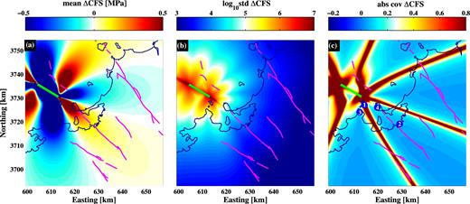
Calculated Coulomb failure stress changes (ΔCFS) with, (a) the mean of the ΔCFS maps, (b) logarithm (base 10) of the standard deviation of the ΔCFS maps and (c) the coefficient of variation (ratio of standard deviation to mean) of the ΔCFS maps, showing high variations between ΔCFS lobes. Blue circles show the locations studied further in Fig. 7. Mapped active faults in the region are shown as magenta lines.
The variability of estimated ΔCFS differs significantly between locations. On Genkai Island (Location 1 in Fig. 6c), which is located close to the source fault where the coefficient of variation of ΔCFS is high, the ΔCFS ranges from −4 to 3 MPa. Estimates of ΔCFS values at such locations near the end of a source fault are usually unreliable as a small change in fault strike can lead to a sign change of the resulting ΔCFS value. Nishinoura (Location 3) and Shika Island (Location 4) both lie in areas where the coefficient of variation is lower (∼0.2) and the 95 per cent confidence interval of the ΔCFS at these locations shows an uncertainty of less than 1 MPa. The Kego fault in Fukuoka city (Location 2) exhibits very low variability with the 95 per cent confidence interval having a width of only 0.025 MPa. The entire distribution of ΔCFS at this location is positive and peaks at ∼0.11 MPa, indicating that all the fault models of the ensemble predict positive ΔCFS on the Kego fault. If the Kego fault extends offshore toward the source fault, then the ΔCFS increase there is even more significant. This is a future concern for Fukuoka city and its current population of more than 1.5 million.
We find that the aftershock locations informative prior affects ΔCFS variations, as the location of positive and negative lobes of ΔCFS are sensitive to the strike of the fault. The high-variation region of ΔCFS that lies along the edges of these lobes can be misplaced if the fault strikes are biased in the fault model estimation (Fig. 5k). As in our case, the strike is constrained better at ∼120° thus reducing the variation of ΔCFS in such regions. The ΔCFS variations at Genkai Island, Shika Island, Nishinoura and Kego fault (Fukuoka city) are lower when using the priors as compared to when not using the priors (Fig. 7). In addition, the ΔCFS values are systematically higher on the Kego fault (Fukuoka city) and under Shika Island when using the informative priors (Figs 7b and 7d).
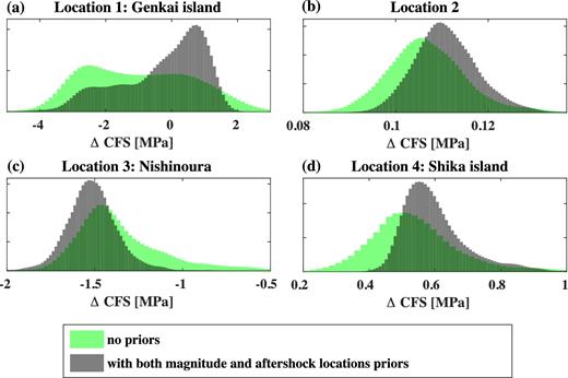
Estimated PDFs of the ΔCFS using priors and without using priors at four locations shown in Fig. 6(c): (a) Genkai island; (b) on the Kego fault in Fukuoka city; (c) Nishinoura and (d) Shika island.
6 DISCUSSION
Many studies have been published on the source parameters of the Fukuoka earthquake as described in Section 2, although all were published without estimated uncertainties. When we compare our fault model parameter results of the earthquake with previous source estimations, we find that some published model parameters fall outside of the error bounds we have estimated (Fig. 8). For example, the NEIC and gCMT centroid locations lie 8 km northwest and 3 km southwest from our solution, respectively, and well outside our 95 per cent confidence ellipse (Fig. 8a). In addition, in all the studies (except one) that used strong motion, GPS and InSAR data to estimate the variable slip distribution, the centroid locations (and the slip asperities) lie southeast of our solution. Only NIED F-net and Ito et al. (2006) have centroid locations within our 95 per cent confidence bounds. The centroid depths of reported solutions also differ considerably, ranging from 10 to 12 km (gCMT, NEIC, NIED F-net and Ito et al.2006) to shallower depths of 4–6 km (Kobayashi et al.2006; Sekiguchi et al.2006; Ozawa et al.2006). The minimum allowed fault depth in the moment tensor solutions (gCMT, NEIC and NIED F-net) is generally 10–12 km (Ekström et al.2012) and hence their fault depth estimates are higher (by about 2-4 km) than the estimates in our study. It is interesting to note that although the aftershock locations prior in our study constrains the fault strike and fault dip, but it does not constrain the fault depth. This is because the aftershock locations are used to constrain an infinite fault plane and thus several vertical fault planes with varying depth that can be subsets of such an infinite fault plane would all have the same aftershock locations prior probability (due to same value of D (m) in eq. 6).

The estimated 1-D/2-D marginal PDFs of several key fault model parameters for the Fukuoka earthquake compared with deterministic solutions reported by several researchers and agencies.
Some of the slip distributions reported in previous studies have more than one slip asperity (Asano & Iwata 2006; Horikawa 2006; Sekiguchi et al.2006). Multiple asperities at different depths are generally not constrained well from geodetic data alone (e.g. Pedersen et al.2003) except for larger earthquakes. Also, fault models using geodetic data have lower resolution for slip at increasing depths. Hence, we simply used a uniform dislocation fault model in this study as the sparse geodetic data do not resolve more than one slip maximum. Moreover, variable and uniform slip models predict similar ΔCFS values at distances far from the fault (Steacy et al.2005). However, using a uniform slip model results in a fault with a shorter length as observed in Section 5.
The moment magnitude estimated in our study peaks at 6.568 and only four solutions lie within the 95 per cent error of our solution. Horikawa (2006) presents an estimate lower than our solution, while other solutions have a slightly higher moment magnitude. The fault strike is well determined in our estimation using the aftershock location prior and peaks at ∼120° with a standard deviation of only ∼1.5 degrees (Fig. 8c). The reported solutions (except for one) have a slightly larger strike value and about half of the solutions lie outside the 1-σ of our results. The fault dip determined is near vertical, dipping slightly to the southwest (Fig. 8d). Most of the published solutions have a similar dip and are within the error bounds, except the NEIC solution dips 63° to the southwest and that of Nishimura et al. (2006) dips 79° to the southwest.
We have shown the importance of priors in our study and proposed a way to estimate hyperparameters, which determine the relative weight between the corresponding prior and the likelihood function. Often, during estimation of slip distribution, slip smoothness priors were used as a regularization term (Jónsson et al.2002; Wright et al.2004) to penalize high slip variations between nearby slip patches. The smoothing/roughness parameter (hyperparameter) has usually been obtained from a trade-off curve of the roughness norm against a weighted residual norm (Du et al.1992; Jónsson et al.2002). A solution was then selected at a roughness parameter value where it falls at the centre of the bend of the curve. Fukuda & Johnson (2008) showed that the location of where such a trade-off curve bends depends on the scaling of the plot axes and thus the choice of roughness parameter may vary with changes in axes scaling. Hence, Fukuda & Johnson (2008) estimated it objectively by sampling the hyperparameter using Bayesian inference, where the hyperparameter that maximized the posterior distribution was chosen. Fukahata & Wright (2008) used ABIC to select the hyperparameters that minimizes the effective cost function by minimizing ABIC and thereby maximizing the marginal likelihood. The estimation of hyperparameters in all of these cases is dependent on the geodetic data and would be affected by changes in the data and their uncertainties. These techniques can be useful when information on the characteristics of the priors is limited or is dependent on the forward model. In contrast, the hyperparameters in our study are not dependent on the forward model and can be estimated solely based on the properties of the prior information. The hyperparameters thus selected are not affected by the geodetic data and their uncertainties.
We estimate the uncertainty of the coseismic ΔCFS at a few locations and observe that ΔCFS can have a multimodal distribution at particular locations and can vary greatly depending on the location around the source fault (Fig. 7a). Thus, a single optimum estimate of the ΔCFS usually reported by authors can be misleading. The ΔCFS estimated at two locations (Locations 2 and 4 in Fig. 7) on the Kego fault are found to be 0.1–0.13 and 0.4–1.0 MPa, respectively. Stein et al. (1997) inferred that nine of 10 earthquakes that occurred on the North Anatolian fault from 1939 to 1992 were brought closer to failure by the preceding earthquakes, typically by ΔCFS of 0.1–1.0 MPa. When secular stress accumulation was included along with coseismic stress change, the mean ΔCFS over the entire future rupture increased by 0.2–0.4 MPa for nine of 10 earthquakes. A similar stress evolution study by Doser & Robinson (2002) showed that six of the seven earthquakes occurring in the Southern Marlborough region (New Zealand) from 1888 to 1994 might have been triggered due to increased ΔCFS (coseismic and secular stress accumulation) of 0.06–0.5 MPa after the previous earthquake. These studies imply that the stress changes caused by the 2005 Fukuoka earthquake on the Kego fault are large enough to significantly advance the next earthquake on that fault. In addition, better information about the interseismic loading rate and stress changes on the Kego fault would improve seismic hazard assessment for Fukuoka city and its surroundings.
7 CONCLUSIONS
In this paper, we have shown how to include a priori information, such as the main shock magnitude and aftershock locations, when constraining earthquake source parameters in Bayesian estimation. This can be useful in cases where geodetic data are limited and do not constrain the fault geometry well. In particular, the aftershock locations prior helps in better constraining the location and strike of the fault. We estimate the hyperparameters that control the weight of a priori information with respect to the likelihood function from the uncertainty of the prior information. This allows the hyperparameters to be independent of the geodetic data and their uncertainties.
Applying this framework to the 2005 Mw6.6 Fukuoka earthquake, we have shown how certain fault model parameters got adjusted to fulfill the a priori constraints, for example fault strike lined up with the aftershock distribution after including the aftershock location information. We propagated the estimated fault model parameters with uncertainties to calculations of ΔCFS, focusing on the Kego fault in Fukuoka city, which is thought to be an extension of the fault activated in the earthquake. We observe that the variability of ΔCFS on the Kego fault is lower when using the priors as against when not using the priors. The results show that the ΔCFS on the Kego fault is strongly positive and hence a concern for the over 1.5 million people living in Fukuoka.
Acknowledgements
We thank Shin'ichi Miyazaki (Kyoto University) for discussions and the Earthquake Research Institute (University of Tokyo) for hosting SJ during the early part of this work. Comments from Yukitoshi Fukahata (Kyoto University) and an anonymous reviewer improved the manuscript. We thank Chiheb Hammouda (King Abdullah University of Science and Technology, KAUST) for fruitful discussions. The ENVISAT data were provided by the European Space Agency through category-1 project 3639. Generic Mapping Tools (GMT) were used to make Fig. 1. This research was supported by KAUST.
REFERENCES
SUPPORTING INFORMATION
Supplementary data are available at GJI online.
Dutta_etal_supplementary.pdf
Figure S1. Time-baseline plot of 21 SAR scenes of the ENVISAT descending track 17 used to select stable point-targets. A scene from January 2005 (index 6) is used for master geometry. The preseismic, coseismic and postseismic pairs are shown that were used to obtain the time series for each stable point-target.
Figure S2. Autocorrelation plots of the MCMC chain of 800000 samples (after combining the Markov chains) for the fault model parameters for the cases: a) using both aftershock locations and moment magnitude as directs priors; b) using aftershock locations as direct prior; c) using moment magnitude as direct prior; d) no direct priors. Based on these autocorrelations, we thin the samples with a lag of 100 to obtain 8000 samples.
Table S1. PSRF values for MCMC samples for 10 Markov chains of the eight fault model parameters. Prs M+AS is when using both aftershock locations and moment magnitude priors; Pr AS using only aftershock locations prior; PrM using only moment magnitude prior; and No Prs using no direct priors.
Please note: Oxford University Press is not responsible for the content or functionality of any supporting materials supplied by the authors. Any queries (other than missing material) should be directed to the corresponding author for the paper.
APPENDIX A: AFTERSHOCK LOCATIONS PRIOR PARAMETERS
In this appendix, we show how different parameters in the aftershock locations prior distribution (in eq. 6) are defined. Consider there are L number of aftershock locations. Using each aftershock location, we define Di(mj) as the perpendicular distance of that ith aftershock from the jth realization of fault model, mj. This is used to form a L-dimensional vector D(mj) such that D(mj) = [D1(mj) D2(mj) … DL(mj)]T. For an ensemble of fault models, m, the distribution of D(m) will be positive valued.
The term, Σl, which is a L × L diagonal matrix, represents the error in D(m) due to errors in the aftershock locations. The error in the aftershocks location is taken as 0.6 km in E-W and N-S directions and 1.6 km in depth (Uehira et al.2006) that results in an ellipsoid of uncertainties around each aftershock location (Fig. A1a). To estimate Σl (in eq. 6), we first estimate the best-fitting fault plane to the aftershock locations. For ith aftershock, we uniformly generate 100 000 sample locations from within the ellipsoid of uncertainty and then calculate Di(m) for these sample locations with the best-fitting fault plane (shown in Fig. A1b). The variance of the resulting Di(m) samples is used as the ith diagonal entry of the Σl error matrix. Σl is used in the estimation of the hyperparameter h22 (Appendix B) and to describe the aftershock locations prior PDF (in eq. 6).
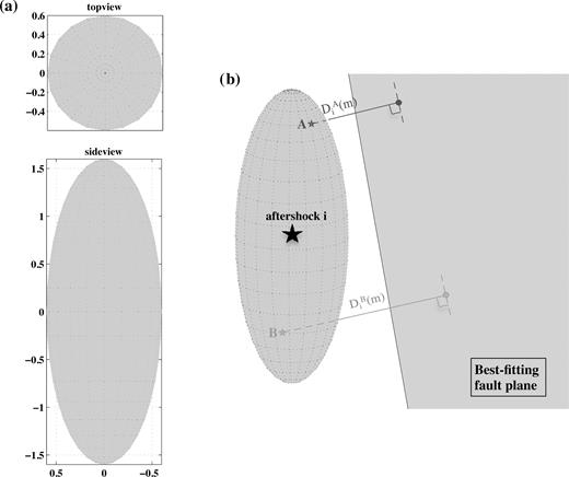
(a) Top and side views of the ellipsoid of uncertainty around each aftershock location depicted as star. (b) Perpendicular distances between the best-fitting fault plane and two sample locations, A and B, within the ellipsoid of uncertainty around ith aftershock.
APPENDIX B: HYPERPARAMETER RELATED TO AFTERSHOCK LOCATIONS PRIOR
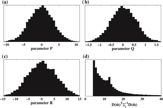
(a)–(c) 1-D marginal posterior PDFs of fault plane model parameters, P, Q and R (in eq. B3). (d) Probability distribution of |$D(\tilde{{\bf m}})^T\Sigma _l^{-1}D(\tilde{{\bf m}})$| estimated from ensemble of fault plane parameters.
