


Summary
The Boring Volcanic Field of the Pacific Northwest (USA), composed of more than 80 eruptive units ranging in age from 3200 to 60 ka, offers a unique possibility to investigate the variability of the Quaternary to late Neogene palaeomagnetic field. To complement previous work on palaeodirections, we conducted 240 absolute palaeointensity (API) experiments with the joint use of the continuous (Wilson) and stepwise (Thellier–Coe) double-heating protocol, along with 620 relative palaeointensity (RPI) experiments based on the pseudo-Thellier approach. We successfully determined absolute estimates for 12 independent eruptive units, as well as relative estimates for 47 out of 132 investigated sites. We compare these results with the existing database for the last 3 Myr and obtain an estimate of the relative variability in palaeointensity on the order of 40–45 per cent as a proxy for palaeosecular variation. API and RPI data suggest a possible asymmetry between normal and reverse polarities.
1 INTRODUCTION
The Earth’s magnetic field is dominated by a strong dipolar component, but also changes stochastically in both direction and intensity though time, which is referred to as secular variation (e.g. Hulot et al. 2010). On decennial, centennial and millennial timescales, palaeosecular variation (PSV) can be reconstructed either from reference curves for a given region (e.g. Hervé et al. 2013a,b) or using time-varying spherical harmonic models (e.g. Nilsson et al. 2014) constrained by direct observations as well as by archaeo- and palaeomagnetic data. The latter approach cannot be applied on multimillion-year timescales because of the sparsity in time and space of data, which are furthermore affected by larger uncertainties. The emphasis is usually placed solely on the reconstruction of a geocentric axial dipole (GAD), which provides as a first approximation an accurate representation of the time-averaged field (e.g. Johnson et al. 2008). In this context, palaeointensity data are usually converted into a virtual dipole moment (VDM), or more often into a virtual axial dipole moment (VADM) when the magnetic inclination is unknown. Time-dependent VADM curves have been published for the past 2 Myr, schematically involving stacking relative palaeointensity (RPI) time-series derived from sedimentary cores and calibrating the resulting curve with absolute palaeointensity (API) determinations derived from volcanic rocks (e.g. Valet et al. 2005; Channell et al. 2009; Ziegler et al. 2011). These reference curves enable, among other things, one to investigate the morphology of reversals and excursions (e.g. Valet et al. 2005), the possible asymmetry between the growth and decay rates of the field (e.g. Ziegler & Constable 2011), as well as the power spectrum of the field (e.g. Constable & Johnson 2005).
In order to better understand the variability of the Earth’s magnetic field, we now focus on the Boring Volcanic Field (BVF), located in the Portland-Vancouver metropolitan area and centred around the city of Boring, USA (Fig. 1). This field comprises an assemblage of late Pliocene and Pleistocene volcanic vents, associated with the subduction of the Juan de Fuca plate beneath western North America (e.g. Evarts et al. 2009). It consists of approximately 80 monogenetic centres that produced subalkaline basalts to basaltic andesites, dated between 59 and 2632 ka. Low-potassium tholeiite flows erupted in the Cascade mountains are also included in this study to extend the time coverage until 3249 ka (e.g. Evarts et al. 2009). 40Ar/39Ar geochronology and palaeomagnetic directions were extensively investigated in Fleck et al. (2014) and Hagstrum et al. (2017) at approximately 150 localities. The aim of our paper is to append palaeointensity results to the directional study.
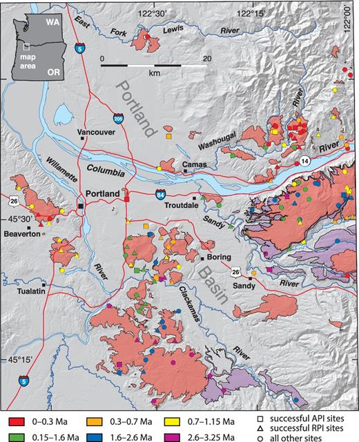
Map showing Boring volcanic rocks in pinkish-orange colour, low-potassium tholeiite flows originating in the Cascade arc to the east in purple, as well as major geographic and cultural features of the region (black squares denote towns and cities and red lines, major roads). Coloured symbols indicate the location of the palaeomagnetic sites as described in the legend. Two sites plot off the map to the east: Site 002 (BL8097) at 45.7549°N, 121.8311°W and Site 013 (T6169) at 45.4156°N, 121.9851°W.
On multimillion-year timescales, PSV is usually quantified by the angular dispersion S of the virtual geomagnetic poles (also known as VGP scatter). As this quantity strongly depends on latitude (e.g. Linder & Gilder 2012), estimates from several latitudes are needed to fully describe the geodynamo state at a given time. Numerical dynamo simulations indicate that the relative variability εF in palaeointensity (standard deviation normalized by the averaged value) correlates well with the geodynamo state and is moreover largely independent of site latitude (Lhuillier & Gilder 2013). This quantity is consequently a useful proxy to describe PSV. One of the aims of this study is to estimate this parameter by coupling API and RPI experiments in order to increase the number of successful determinations.
In this paper, we first describe the experimental methods employed for the determination of rock-magnetic properties, palaeodirections and palaeointensities. We then present our results, emphasizing in particular how we selected the most suitable specimens for palaeointensity experiments, how we filtered the most reliable palaeointensity estimates and how we empirically calibrated the RPI determinations. We finally discuss the robustness of the pseudo-Thellier method and compare our results with the existing database.
2 METHODS
2.1 Sampling
Oriented palaeomagnetic core samples of BVF lavas were collected primarily from artificial (e.g. road and quarry) and stream cut exposures in order to obtain the freshest possible rock (Fleck et al. 2014; Hagstrum et al. 2017). At most sites, eight samples were drilled and oriented using an orienting tool that included both magnetic and solar compasses, and a clinometer. Samples for geochronology were usually collected at the same outcrop, although some outcrops were deemed less suitable for 40Ar/39Ar dating due to thin-section examinations that showed fine grain size, glassy groundmass and/or weathering. In such cases, samples were collected from other parts of the same flow as best determined by field relationships or by petrographic and geochemical analyses.
For this study, we investigated 132 out of the 136 sites reported in Hagstrum et al. (2017), which comprise 77 independent eruptive units. Five palaeomagnetic specimens (1-in. cores) were at our disposal for each site, for a total of 640 specimens. To allow a higher variety of experiments, each specimen was divided as follows. We first drilled an 8.8 mm diameter core in the centre of each specimen. We then cut the remaining 1-in. core into two equally high cylinders, named A for the upper part, B for the lower part. The 8.8 mm diameter core was subsequently divided into two equally high cylinders, named C for the upper part and D for the lower part.
2.2 Rock-magnetic analysis
For one A-specimen from each site, rock-magnetic measurements were carried out at the Ludwig-Maximilians-University of Munich on a 5-mm subcore. Continuous thermomagnetic curves were measured on a Petersen Instruments variable field translation balance, while heating in air from room temperature to 600 °C using a field of approximately 200 mT. The Curie point TC was determined as the temperature corresponding to the maximum of the first-time derivative (e.g. Fabian et al. 2013). Hysteresis and backfield curves were made with a one-component Lakeshore vibrating sample magnetometer (VSM). The hysteresis loops were corrected for the paramagnetic contribution by the slope above 0.5 T. From these measurements, standard hysteresis parameters—saturation magnetization (MS), remanent saturation magnetization (MRS), coercive force (HC) and remanent coercive force (HCR)—were calculated and the hypothetical domain structure was estimated from the Day et al. (1977) plot using the ratios MRS/MS and HCR/HC. Additional analyses of the mineral composition were made with an STOE STADI multipurpose X-ray powder diffractometer (cobalt Kα1 radiation) at the Geophysical Observatory of Borok. Magnetic susceptibilities χm were finally measured before demagnetization using a Bartington MS2B meter operating at a frequency of 0.465 kHz.
2.3 Directional analysis
A-specimens were alternating field (AF) demagnetized up to 90 mT with the aid of the automated SushiBar system based on a three-axis 2G Enterprises superconducting magnetometer and a custom-made coil in the magnetically shielded room at Munich University (Wack & Gilder 2012). The median destructive field (MDF)—the value for which half of the initial natural remanent magnetization (NRM) is randomized—was computed for each sample from the decay curve reconstructed by modular subtraction. Thermal demagnetizations were carried out on one of the five B-specimens for each site, using an ASC TD-48 furnace together with an AGICO JR6 spinner magnetometer. The specimen-level characteristic remanent magnetization (ChRM) direction was determined using principal component analysis (PCA, Kirschvink 1980) or, in exceptional cases, the great circle method (McFadden & McElhinny 1988) with the help of the paleomagnetism.org environment (Koymans et al. 2016). The mean directions were then calculated according to Fisher (1953) statistics.
2.4 Absolute palaeointensity experiments
At the Borok Observatory, 40 Wilson and 40 Thellier palaeointensity experiments were carried out on pilot C- and D-specimens using a custom-made, fully automated three-component VSM, which operates with a sensitivity of 10−8Am2 (e.g. Shcherbakova et al. 2012, 2014, 2017). Additional Thellier palaeointensity experiments (160) were processed on 5-mm subcores of the B-specimens in the magnetically shielded room at Munich, using an ASC TD-48 furnace together with an AGICO JR6 spinner magnetometer.
The Wilson (1961) method compares a specimen’s continuous thermal demagnetization curve of the NRM with that of a full thermoremanent magnetization (TRM) induced in a known laboratory field Blab (50 μT in our case). Within a temperature interval, chosen as close as possible to the interval where the ChRM was isolated, the proportionality coefficient kp between the NRM and TRM can be fitted with its relative standard error (RSE). The palaeointensity estimate Banc is finally given by kp × Blab.
The Thellier & Thellier (1959) method replaces in progressive stages a specimen’s NRM with partial TRMs (pTRMs) induced in a known laboratory field Blab (50 μT in our case). The experiments were made according to the double-heating protocol of Coe (1967) with pTRM checks. The statistics of the Thellier experiments were computed according to standard definitions: n, the number of points used for the best-fit line on the Arai–Nagata diagram (Nagata et al. 1963); f, the NRM fraction used for the best-fit line on the Arai–Nagata diagram; β, the standard value of the slope normalized by its absolute value; q, the quality factor (Coe et al. 1978); |$\mathit {\text{MAD}}$|, the maximum angular deviation of the origin-anchored directional fits (Kirschvink 1980); α, the angular difference between the origin-anchored and free-floating best-fit directions; |$\mathit {\text{DRAT}}$|, the maximum difference ratio measured from pTRM checks (Selkin & Tauxe 2000); and |$\mathit {\text{CDRAT}}$|, the sum of the absolute pTRM differences (Kissel & Laj 2004).
2.5 Relative palaeointensity experiments
The pseudo-Thellier analysis (Tauxe et al. 1995) is an RPI method, recently applied to volcanic rocks (e.g. de Groot et al. 2013). The first stage involves the stepwise AF demagnetization of a specimen’s NRM. It was performed in 5 mT steps up to 50 mT, then in 10 mT steps up to 90 mT. For the same specimen, the second stage involves the stepwise acquisition of an anhysteretic remanent magnetization (ARM) in a known laboratory field Blab (50 μT in our case). The third stage is the stepwise AF demagnetization of the last imparted ARM (the one with a peak field of 90 mT in our case). This last stage compares the demagnetization spectra of the natural and laboratory-imparted remanences to assess whether they operate within the same coercivity range. To account for the variable amounts of NRM remaining after the 90 mT step, we removed by vector subtraction the residual magnetization from all remanence data. This can be a posteriori validated by checking that RPI determinations are uncorrelated with the residual magnetization (Fig. S1, Supporting Information).
The results are then analysed in the framework of a pseudo-Arai diagram that compares the remaining NRM with the acquired ARM. The slope b between these two quantities over the chosen AF segment—computed in the sense of Coe et al. (1978) with its standard deviation σb, NRM fraction f and relative standard error β—yields the RPI estimate. To check the reliability of the estimates, the pseudo-Arai diagram can be supplemented with a demag–demag plot (ARM remaining versus NRM remaining) as well as an ARM–ARM plot (ARM remaining versus ARM gained), according to Paterson et al. (2016). Both diagrams are expected to yield straight lines over the chosen segment, with the additional constraints that the best-fit line on the demag–demag plot should intersect the origin and the slope on the ARM–ARM plot should tend towards unity. The linearity (respectively the trend towards the origin) can be quantified by the coefficient R of correlation (respectively the fraction fres of residual ARM at the origin). To take into account that the pseudo-Thellier analysis is a relative method and dependent on the size distribution of the remanence-carrying grains (e.g. Yu et al. 2003), the accepted RPI estimates must be carefully selected. We follow de Groot et al. (2013) by selecting samples whose grain-size indicator BARM1/2—the AF field for which half of the maximum ARM is imparted—is limited to the range of 20–60 mT.
3 RESULTS
3.1 Preliminary analysis
For the 640 specimens investigated in this study, the distribution of NRM values is approximately lognormal (Fig. 2a), ranging from 0.1 to 22.0 A m−1, with a median value of 2.2 A m−1. The Koenigsberger ratio Q, which is the ratio of the remanent magnetization to the induced magnetization (χm × B/μ0), was computed for a magnetic field B = 54 μT in 2001 at Boring (Maus et al. 2005), where μ0 is the magnetic constant. Its distribution is also roughly lognormal (Fig. 2b), ranging from 0.2 to 113.6, with a median value of 4.3. The MDF from the AF demagnetization curves ranges from 2.7 to 86.4 mT, with a median value of 27.3 mT. Fig. 2(c) shows a positively skewed and multimodal distribution that does not correlate with NRM or Q values (Figs 2a and b). A kernel smoothing fitting function with a bandwidth of 3 mT reveals two main maxima at approximately 11 and 29 mT.
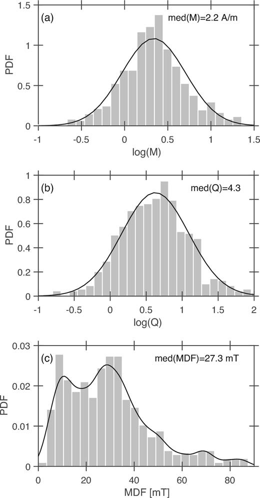
Preliminary analysis of the results: (a) empirical distribution of the NRMs with a lognormal fit; (b) empirical distribution of the Koenigsberger ratios Q with a lognormal fit; (c) empirical distribution of the MDFs with a kernel smoothing fit (bandwidth of 3 mT). The median values are provided for each of the distributions.
3.2 Rock-magnetic analysis
As illustrated in Figs 3(a) and 4, our thermomagnetic results can be categorized into three groups. Group 1 (67 per cent of the specimens) is characterized by a narrow range of single pronounced Curie temperatures (TC) between 440 °C and 560 °C (median of 533 ± 23 °C). Heating and cooling branches often show good reversibility indicating that limited alteration occurred. Group 2 (12 per cent of the specimens) is characterized by a range of single pronounced Curie temperatures between 100 °C and 300 °C (median of 149 ± 52 °C). Heating and cooling branches in most cases are entirely dissimilar. Group 3 (21 per cent of the specimens) is more heterogeneous and characterized by two ferrimagnetic phases: one with a low TC in the range 150–350 °C (232 ± 64 °C); another with a higher TC between 450 °C and 550 °C (505 ± 33 °C). Heating and cooling branches are in the majority of cases not reversible.
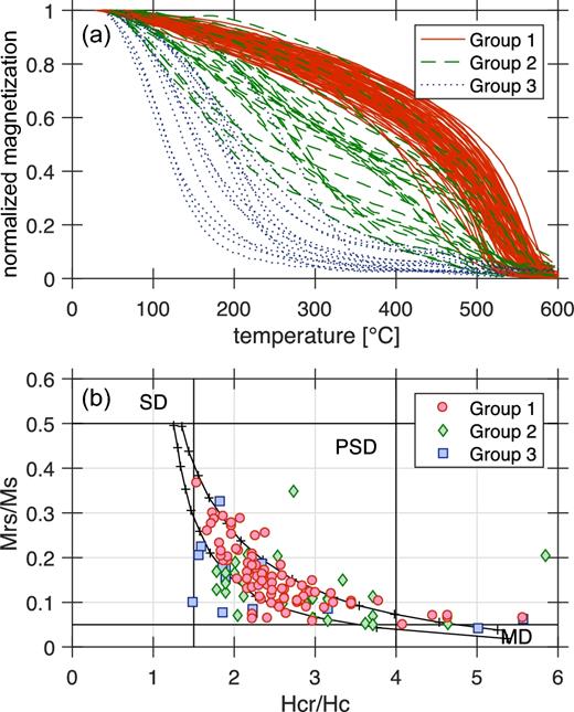
Overview of the rock-magnetic properties: (a) heating branches of the thermomagnetic curves; (b) Day plot with SD and MD mixing curves of pure magnetite (Dunlop 2002). The three colours account for the three groups defined in the text: Group 1 in red with high TC, Group 2 in blue with low TC and Group 3 in green with two ferrimagnetic phases.
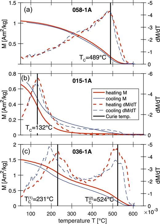
Typical thermomagnetic curves: (a) specimen 058-1A from Group 1 with high TC; (b) specimen 015-1A from Group 2 with low TC; (c) specimen 036-1A from Group 3 with two ferrimagnetic phases. The black vertical lines indicate the Curie temperatures TC estimated from the derivative of the heating branches.
The bulk hysteresis properties, shown in a Day plot (Fig. 3b), reveal that most of the specimens lie in the area normally associated with pseudo-single domain behaviour. Specimens from Groups 2 and 3 display the highest dispersion with a trend towards a higher HCR/HC for Group 3 than for Group 2. Specimens from Group 1 evolve within a well-constrained area between the single domain (SD) and multidomain (MD) mixing curves of pure magnetite (Dunlop 2002).
In order to identify the mineralogical composition of ferrimagnetic grains, the magnetic fractions from a few specimens were subjected to X-ray structural analysis at room temperature. Specimens from Group 1 contain exsolved (high-temperature exsolution lamellae) slightly oxidized low-titanium magnetite (∼60 per cent) and cation substituted haematite (∼40 per cent), whereas specimens from Groups 2 and 3 display wide asymmetric lines that are indicative of compositionally heterogeneous titanomagnetite (Fig. S2, Supporting Information). For titanomagnetite Fe3−xTixO4, the ulvospinel content x and oxidation parameter z (fraction of original Fe2 + converted to Fe3 +) were estimated from the lattice constant a and Curie temperature TC (Nishitani & Kono 1983). Specimens from Group 1 yielded z ≈ 0.3, whereas the oxidation parameter was twice higher for the other groups (Table 1). These observations are in good accordance with the thermomagnetic curves. They confirm that the specimens from Group 1, with thermally stable slightly oxidized low-titanium magnetite, are well suited for API experiments, whereas the specimens from the other groups are thermally unstable.
Crystallography of select titanomagnetite specimens: lattice constant a and Curie temperature TC; ulvospinel content x and oxidation parameter z estimated from Nishitani & Kono (1983).
| Specimen (group) | a (nm) | TC (°C) | x | z |
|---|---|---|---|---|
| 006-2 (3) | 0.8444 | 282 | 0.7 | 0.6 |
| 008-2 (1) | 0.8384 | 499 | 0.2 | 0.3 |
| 029-2 (1) | 0.8383 | 544 | 0.1 | 0.3 |
| 048-2 (1) | 0.8387 | 546 | 0.1 | 0.3 |
| 063-2 (2) | 0.8442 | 294 | 0.7 | 0.6 |
| Magnetite | 0.8396 | 585 | – | – |
3.3 Directional analysis
For all specimens, with the exception of the five sites mentioned hereinafter, the ChRM direction was unambiguously determined using PCA with best-fit lines forced to the origin. Sister specimens subjected to both thermal and AF demagnetizations yielded virtually identical ChRM directions. Fig. 5 presents two typical examples of thermal and AF demagnetized sister specimens. For Sites 008 (T3004) and 023 (T3028), the PCA lines were unanchored to account for some AF demagnetized specimens that did not trend towards the origin (Figs S3a and b, Supporting Information). For a few specimens from Sites 019 (T3044), 020 (T3052) and 025 (T5017), the great circle method was employed, whereas the other specimens were fitted using PCA (Figs S3c and d, Supporting Information).
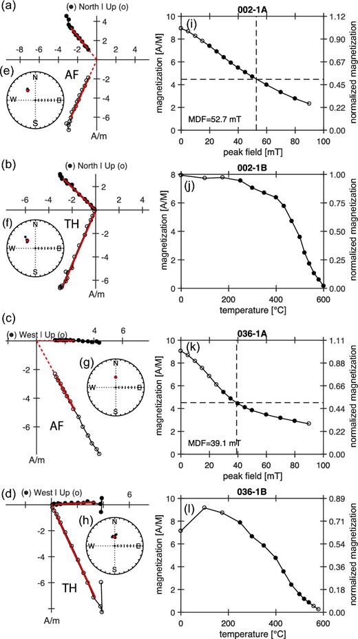
Typical behaviour of thermal and AF demagnetized sister specimens: (a)–(d) orthogonal plots; (e)–(h) stereographic plots; (i)–(l) decay plots. The median destructive field (MDF) corresponds to the AF field for which half of the initial NRM is randomized. The PCA directions are highlighted in red.
For each site, the newly acquired directions were compared to those reported in Hagstrum et al. (2017). The two data sets proved to be nearly indistinguishable with an angular distance δ lower than 5° for 80 per cent of the sites (Fig. S4, Supporting Information). Four sites had angular distances higher than 15°: Sites 030 (T3383), 074 (4T128) and 129 (4T208) contained different sample sets between Hagstrum et al. (2017) and this study that yielded different directional populations; Site 055 (BL8041) had an outlying direction that was retained in Hagstrum et al. (2017), but removed in this study.
Table S1 in the Supporting Information reports the intrasite directional parameters that were recomputed by combining the individual directions of the previously and newly acquired measurements. Sites 048 (T5153) and 049 (BL9001) lie within the Brunhes–Matuyama transition, whereas Sites 055 (BL8041) and 057 (T2295) lie within the Matuyama–Jaramillo transition. Removing these transitional sites and grouping the sites by eruptive units, we obtain the distribution of directions and VGPs in Fig. 6. The between-site dispersion SB of VGPs, corrected for within-site dispersion (e.g. Johnson et al. 2008), with 95 per cent confidence limits (Cox 1969), yields |$22.82^{\circ }(_{19.66^{\circ }}^{27.20^{\circ }})$| (N = 38) for the normal polarities, |$15.37^{\circ }(_{13.24^{\circ }}^{18.32^{\circ }})$| (N = 38) for the reversed polarities and |$19.32^{\circ }(_{17.36^{\circ }}^{21.79^{\circ }})$| (N = 76) for the combined polarities. In accordance with Hagstrum et al. (2017), the dispersion is approximately 30 per cent higher for the normal polarities than for the reversed polarities, whereas the dispersion for the combined polarities lies within the range of the values predicted by the TK03.GAD field model (Tauxe & Kent 2004). The Brunhes and Matuyama chrons yield |$S_B=22.80^{\circ }(_{19.19^{\circ }}^{28.08^{\circ }})$| (N = 28) and |$S_B=17.07^{\circ }(_{14.71^{\circ }}^{20.35^{\circ }})$| (N = 38), respectively.
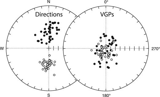
Directions and VGPs grouped by eruptive units.
3.4 Absolute palaeointensity determinations
Based on the thermomagnetic curves, we selected a set of 40 specimens, for which the heating and cooling cycles showed good reversibility: 30 from Group 1, 8 from Group 2 and 2 from Group 3. Wilson experiments showed that all the specimens from Groups 2 and 3 failed to yield robust palaeointensity estimates, producing sometimes a partial self-reversal during the demagnetization of the TRM (Figs 7d and f). This partial self-reversal was however not seen during the demagnetization of the NRM, indicating that a transformation happened during the first heating cycle. The specimens from Group 1 passed the empirical criterion of RSE ≤ 0.02 (Muxworthy 2010) in approximately 30 per cent of the cases. An example of a successful experiment is shown in Figs 7(a)–(c), whereas the detailed results are reported in Table S2 in the Supporting Information.
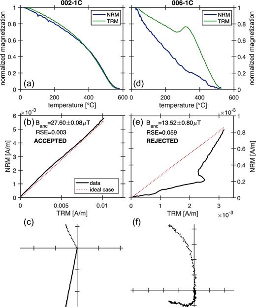
Examples of Wilson experiments: (a) and (d) NRM and TRM as a function of temperature; (b) and (e) remaining NRM versus remaining TRM; (c) and (f) orthogonal plot of the NRM (arbitrary orientation).
Based on these preliminary results, Thellier experiments were carried out on a set of 200 specimens, both using a three-component VSM (40 specimens) and a palaeointensity furnace (160 specimens). The two apparatuses gave nearly indistinguishable results. Those from the Thellier experiments can be schematically classified into three categories according to their behaviour on the Arai–Nagata diagram: (i) the specimens that produced a single linear slope over most of the temperature spectrum (Figs 8a and b); (ii) the specimens that produced two linear slopes—a steep one up to approximately 500 °C followed by a more moderate one up to approximately 600 °C (Fig. 8c); (iii) the specimens that produced a concave slope (Fig. 8d), characteristic of alteration or MD behaviour (e.g. Shcherbakov & Shcherbakova 2001). The specimens from the third category were immediately rejected. The specimens from the second category were only retained when we had the insurance that the slope was fitted within a temperature range akin to that used to determine the directions. The specimens from the first category were almost always retained. Based on this heuristic approach, we determined a palaeointensity estimate on 87 out of the 200 specimens (Table S3, Supporting Information). We then selected a more robust set of 54 palaeointensity estimates passing the following selection criteria: n ≥ 4; β ≤ 0.1; q ≥ 5; f ≥ 0.4, |$\mathit {\text{MAD}}\le 10^{\circ }$|; α ≤ 15°, |$|\mathit {\text{DRAT}}|\le 15$| per cent and |$|\mathit {\text{CDRAT}}|\le 15$| per cent.
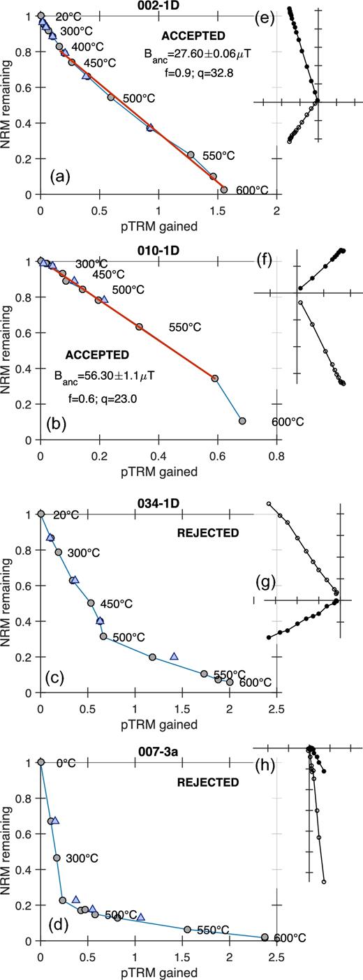
Examples of Thellier–Coe experiments: (a)–(d) normalized Arai–Nagata diagrams; (e)–(h) orthogonal plots (arbitrary orientation). The blue triangles represent the pTRM checks.
As the individual Thellier and Wilson experiments yielded consistent results without any systematic trend (Fig. 9a), so we calculated site-mean palaeointensity estimates of the combined Wilson and Thellier measurements. We obtained 12 (respectively 10) mean estimates before (respectively after) the application of the selection criteria (Table 2). Each of them corresponds to an independent eruptive unit. Over an investigated period ranging from 95 to 3074 ka, the present results yield a time-averaged palaeointensity estimate of 32.0 ± 14.7 μT (respectively 33.7 ± 14.5 μT) before (respectively after) the application of the selection criteria.
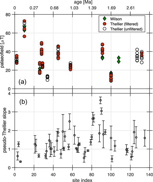
Absolute and relative palaeointensity results: (a) palaeofield as a function of the age (or site index) for the Wilson and Thellier–Coe experiments; (b) pseudo-Thellier slope with 1σ error as a function of the age (or site index).
Absolute palaeointensity estimates Banc (μT) per site and associated virtual dipole moment (VDM) in 1022Am2. The values between brackets correspond to the values after the application of the selection criteria.
| Site | Age (ka) | n | Banc | σ(Banc) | VDM |
|---|---|---|---|---|---|
| 002 (BL8097) | 95 ± 9 | 7(4) | 30.9(31.5) | 2.8(3.7) | 5.7(5.8) |
| 010 (T0260) | ∼134 | 7(5) | 66.0(64.7) | 5.5(6.0) | 1.2(1.1) |
| 026 (T5025) | 281 ± 5 | 9(9) | 21.4(21.4) | 4.5(4.5) | 3.0(3.0) |
| 028 (BL8073) | 339 ± 3 | 11(11) | 41.6(41.6) | 3.9(3.9) | 7.1(7.1) |
| 029 (T2271) | 344 ± 5 | 9(6) | 25.7(26.0) | 1.7(1.7) | 5.0(5.0) |
| 034 (T8073) | 607 ± 22 | 7(0) | 12.4(–) | 1.4(–) | 2.2(–) |
| 045 (BL8113) | 766 ± 5 | 10(7) | 39.1(37.7) | 4.3(4.2) | 6.3(6.1) |
| 058 (T5073) | ∼1031 | 9(6) | 24.1(23.3) | 2.3(2.0) | 5.0(4.8) |
| 091 (T3256) | 1585 ± 16 | 8(8) | 40.7(40.7) | 5.5(5.5) | 7.5(7.5) |
| 100 (T6279) | 1694 ± 13 | 11(11) | 12.4(12.4) | 2.9(2.9) | 2.0(2.0) |
| 127 (T3104) | 2632 ± 9 | 7(0) | 35.0(–) | 4.3(–) | 6.6(–) |
| 132 (T5192) | 3074 ± 18 | 7(2) | 34.5(37.3) | 4.0(1.9) | 4.6(5.0) |
| Mean | – | 12(10) | 32.0(33.7) | 14.7(14.5) | 5.5(5.8) |
3.5 Relative palaeointensity determinations
Pseudo-Thellier analyses were carried out on the whole set of A-specimens, which yielded 622 determinations from 132 sites and 77 independent eruptive units. The pseudo-Thellier slope b and associated parameters were calculated over the 30–70 mT coercivity range, which lies within the range of AF segments that were chosen for the directional analyses. We initially omitted the data from 49 specimens, whose AF demagnetization curves did not trend towards the origin or were incompatible with the site-mean direction. We then applied technical selection criteria—R2 > 0.95 for the pseudo-Arai, demag–demag and ARM–ARM diagrams, f > 0.30 and fres < 0.20—together with a physical constraint on the grain-size indicator BARM1/2 such that it covered the range of 20–60 mT. This yielded a set of 253 measurements shared among 88 sites and 60 eruptive units. A typical example of successful pseudo-Thellier experiment is shown in Fig. 10, whereas the full details are reported in Table S4 in the Supporting Information.
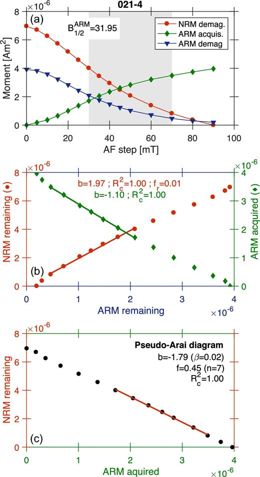
Typical example of a successful pseudo-Thellier experiment: (a) magnetization diagram; (b) combined demag–demag and ARM–ARM diagrams; (c) pseudo-Arai diagram that provides the relative palaeointensity estimate b with it normalized standard error β. The straight lines are fit on the 30–70 mT coercivity range. See Section 2 for a full description of the parameters.
Averages were computed for each site when more than three determinations were available. We additionally disregarded sites for which the relative uncertainty on the average value was greater than 50 per cent. This led to robust RPI estimates for 47 out of 132 sites. The results are reported in Table 3 and summarized in Fig. 9(b). We obtain an intersite averaged pseudo-Thellier slope of −1.36 ± 0.69. With bootstrap experiments on 1000 draws (Fig. S5c, Supporting Information), the relative variability εF is estimated at 50 ± 5 per cent. It reduces to 44 ± 5 per cent when the sites of same age are combined.
Relative palaeointensity estimates per site: pseudo-Thellier slope b (estimate of relative palaeointensity); grain-size indicator BARM1/2 (AF field for which half of the maximum ARM is imparted); virtual dipole moment (VDM) expressed in 1022Am2.
| Site | Age (ka) | n | b ± σ | BARM1/2 ± σ | VDM |
|---|---|---|---|---|---|
| 003 (T2287) | 108 ± 6 | 5 | −0.6 ± 0.2 | 31.3 ± 6.1 | 3.96 |
| 004 (4T064) | 108 ± 6 | 3 | −1.3 ± 0.1 | 28.0 ± 4.6 | 7.30 |
| 006 (T5049) | 116 ± 9 | 5 | −0.3 ± 0.0 | 23.9 ± 0.9 | 2.80 |
| 021 (T5033) | 270 ± 12 | 3 | −1.3 ± 0.5 | 26.9 ± 5.5 | 4.58 |
| 022 (T0285) | 272 ± 11 | 4 | −1.2 ± 0.3 | 32.9 ± 1.9 | 5.04 |
| 025 (T5017) | 281 ± 5 | 3 | −0.6 ± 0.1 | 23.1 ± 3.1 | 2.71 |
| 032 (T5294) | 611 ± 28 | 3 | −0.6 ± 0.1 | 21.2 ± 0.9 | 3.68 |
| 033 (T8089) | 616 ± 21 | 3 | −0.9 ± 0.4 | 29.6 ± 6.4 | 5.48 |
| 036 (T5302) | 662 ± 8 | 4 | −1.5 ± 0.4 | 23.1 ± 1.4 | 6.02 |
| 037 (BL8129) | 662 ± 8 | 3 | −1.0 ± 0.4 | 31.7 ± 8.1 | 5.28 |
| 038 (A3001) | 675 ± 18 | 3 | −1.0 ± 0.3 | 28.7 ± 2.9 | 6.08 |
| 041 (A3013) | 678 ± 22 | 3 | −0.9 ± 0.3 | 29.5 ± 2.4 | 5.44 |
| 044 (T5278) | 766 ± 5 | 5 | −1.4 ± 0.5 | 22.4 ± 1.0 | 5.51 |
| 045 (BL8113) | 766 ± 5 | 4 | −1.9 ± 0.2 | 24.7 ± 1.2 | 7.60 |
| 048 (T5153) | 778 ± 4 | 3 | −0.7 ± 0.2 | 25.6 ± 1.3 | 4.08 |
| 050 (A3061) | ∼833 | 4 | −1.9 ± 0.9 | 28.8 ± 5.5 | 6.57 |
| 051 (4T104) | 875 ± 6 | 5 | −1.0 ± 0.1 | 45.3 ± 4.2 | 5.43 |
| 052 (4T040) | 880 ± 17 | 3 | −1.7 ± 0.3 | 26.9 ± 1.1 | 6.63 |
| 056 (4T256) | 1011 ± 28 | 5 | −1.1 ± 0.2 | 27.3 ± 0.8 | 4.85 |
| 057 (T2295) | 972 ± 3 | 4 | −2.5 ± 0.4 | 29.7 ± 2.3 | 8.71 |
| 062 (T6217) | 1063 ± 9 | 4 | −1.8 ± 0.5 | 27.9 ± 4.1 | 8.57 |
| 064 (4T017) | 1149 ± 3 | 3 | −1.0 ± 0.0 | 26.3 ± 2.2 | 4.56 |
| 065 (4T096) | 1149 ± 3 | 5 | −0.9 ± 0.1 | 25.0 ± 4.5 | 4.65 |
| 066 (4T192) | 1149 ± 3 | 5 | −1.2 ± 0.4 | 23.9 ± 0.9 | 5.31 |
| 067 (4T072) | 1149 ± 14 | 3 | −1.3 ± 0.1 | 22.3 ± 1.4 | 6.88 |
| 072 (T2231) | 1217 ± 4 | 4 | −0.5 ± 0.2 | 25.0 ± 0.9 | 3.26 |
| 073 (T3088) | 1217 ± 4 | 5 | −0.8 ± 0.2 | 25.0 ± 1.6 | 3.32 |
| 076 (A3049) | 1230 ± 10 | 4 | −0.9 ± 0.0 | 22.6 ± 0.4 | 4.70 |
| 079 (T2279) | 1300 ± 19 | 5 | −1.4 ± 0.1 | 29.6 ± 1.3 | 6.53 |
| 080 (T5145) | 1390 ± 8 | 3 | −1.7 ± 0.1 | 27.4 ± 0.9 | 7.99 |
| 081 (T3280) | 1422 ± 21 | 4 | −2.6 ± 0.4 | 26.5 ± 3.1 | 10.88 |
| 082 (T5169) | 1422 ± 21 | 5 | −2.7 ± 0.2 | 31.9 ± 2.3 | 10.42 |
| 088 (T2255) | 1585 ± 16 | 3 | −1.9 ± 0.5 | 24.0 ± 3.5 | 8.46 |
| 089 (T3060) | 1585 ± 16 | 5 | −3.6 ± 0.2 | 31.4 ± 1.0 | 16.19 |
| 090 (T3068) | 1585 ± 16 | 3 | −3.0 ± 0.2 | 28.4 ± 1.2 | 13.19 |
| 092 (4T112) | 1585 ± 16 | 3 | −1.8 ± 0.7 | 24.3 ± 3.8 | 7.86 |
| 094 (4T248) | 1585 ± 16 | 4 | −1.9 ± 0.1 | 27.3 ± 0.7 | 9.96 |
| 100 (T6279) | 1694 ± 13 | 3 | −1.6 ± 0.6 | 35.5 ± 8.4 | 6.62 |
| 101 (BL9010) | 1702 ± 8 | 5 | −0.5 ± 0.2 | 24.7 ± 0.7 | 2.95 |
| 104 (4T167) | 2236 ± 32 | 5 | −1.2 ± 0.3 | 26.3 ± 0.8 | 5.40 |
| 116 (4T224) | 2585 ± 10 | 4 | −1.0 ± 0.3 | 31.4 ± 1.1 | 5.52 |
| 117 (T3120) | 2596 ± 19 | 3 | −0.9 ± 0.1 | 27.1 ± 6.8 | 4.80 |
| 121 (T3153) | 2618 ± 57 | 3 | −0.6 ± 0.2 | 22.9 ± 3.2 | 3.53 |
| 122 (T5089) | 2618 ± 57 | 5 | −0.9 ± 0.3 | 30.7 ± 3.0 | 5.35 |
| 124 (4T120) | 2623 ± 42 | 5 | −1.9 ± 0.6 | 32.7 ± 4.3 | 8.54 |
| 126 (T3096) | 2632 ± 9 | 3 | −1.6 ± 0.6 | 25.8 ± 1.4 | 7.94 |
| 135 (T5113) | 3124 ± 42 | 5 | −1.6 ± 0.4 | 23.9 ± 1.9 | 7.44 |
| Mean | – | 47 | −1.5 ± 0.7 | 27.5 ± 4.3 | 6.4 ± 2.7 |
3.6 Behaviour of the dipolar field
4 DISCUSSION
4.1 Distribution of the VADMs
API data from the last 5 Myr are archived in global databases.1,2 For our analysis, we use the world palaeointensity database (WPD) maintained by the Borok Geophysical Observatory (e.g. Shcherbakov & Sycheva 2013; Shcherbakov et al. 2014) that includes all known published results of reconstructed dipole strength (in terms of VDM or VADM) obtained from eruptive or baked rocks. For the last 3 Myr, it consists of 1974 average estimates, which reduce to 570 estimates after applying the selection criteria of Perrin & Shcherbakov (1997): at least three individual determinations for each average estimate, an uncertainty lower than 15 per cent and the use of a check-point procedure. Fig. 11(a) shows the histograms of VADMs from the filtered and unfiltered database. These distributions are compared in Fig. 11(b) with those derived from the Sint-2000 composite curve (Valet et al. 2005) and the PADM2M field model (Ziegler et al. 2011) for the past 2 Myr, as well as the PISO-1500 composite curve (Channell et al. 2009) for the past 1500 kyr. The database and the PISO-1500 curve show comparable distributions, whereas the Sint-2000 and PADM2M curves display lower average values and narrower distributions. It indicates that the Sint-2000 and PADM2M curves underestimate the true variability, or that the database and the PISO-1500 curve overestimate it. This study produces a set of API determinations whose average is centred on the maximum likelihood of the Sint-2000 distribution (Fig. 11b).
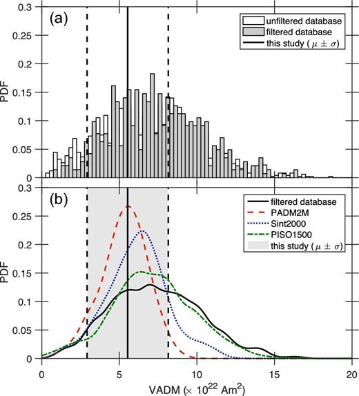
Distribution of the virtual axial dipole moment (VADM) for the last 3 Myr: (a) from the filtered and unfiltered palaeointensity database; (b) from the filtered database and three reference curves (kernel smoothing fit with a bandwidth of 5 × 10²¹ Am2). Vertical lines represent the average value (with its standard deviation) of this study’s API determinations.
4.2 Time evolution of the VADMs
Fig. 12 compares the time variability of our palaeointensity determinations with the filtered database (panel a) and the Sint-2000 composite curve (panel b). At first appearance, our API and RPI data show nothing but random variations about the Sint-2000 curve. One can however note a trend towards lower values during the Brunhes chron. For the BVF, this observation is accompanied by a VGP scatter that is 25 per cent higher during the Brunhes than the Matuyama chron. Another distinctive feature only seen in RPI data is an interval of high intensity with negative inclination around 1.6 Ma during the C1r.3r chron. This deviation does not appear in the filtered database, but is present in the unfiltered database. This period deserves more investigation to discern whether it reflects a geomagnetic feature or stems from an experimental artefact. Fig. 12(d) shows the VADM of our data set as a function of inclination. It reveals a higher dispersion in inclination for normal polarities, in contrast with a higher dispersion in intensity for reverse polarities.
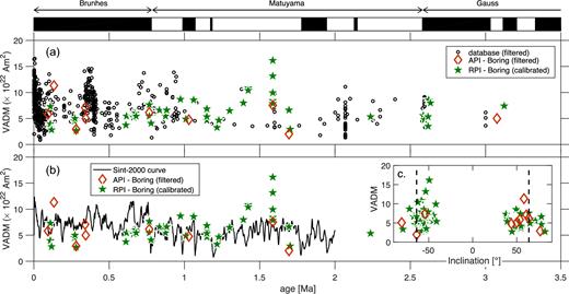
Dipole moment over the last 3 Myr: this study’s API and RPI estimates compared with (a) the filtered database and (b) the Sint-2000 composite curve. (c) Inclination as a function of age.
Special attention must be paid to the fact that the RPI estimates required a calibration to be converted into VADM. Our calibration relies on the theoretical assumption that the API and RPI determinations satisfy the same distribution function, which could not be internally verified due to the restricted number of API results. However, RPI estimates are consistent with the API estimates. It gives hope that the pseudo-Thellier method can provide additional insight into the Earth’s magnetic field variability, but also underlines the necessity of intercomparisons with other methods to better assess its reliability and uncertainty (e.g. Paterson et al. 2016).
4.3 Estimation of the relative variability εF
The relative variability εF in palaeointensity is a robust PSV proxy, whose main advantage is its weak dependency on site latitude (Lhuillier & Gilder 2013). In other words, it can be directly compared with other sections at any site location, whereas the VGP scatter can only be compared at a given site latitude. The quantity εF can be estimated from uncalibrated RPI determinations, without requiring an absolute methodology that suffers from a lower success rate. For the Boring volcanics, we obtain a raw estimate εF = 50 ± 5 per cent (N = 47), which reduces to εF = 44 ± 5 per cent (N = 34) when combining sites of the same age. This compares well with the 0–3 Myr database that yields εF = 49 ± 1 per cent (N = 1974) in the unfiltered case or εF = 42 ± 1 per cent (N = 570) in the filtered case (Fig. S7, Supporting Information). The reference curves PADM2M, Sint-2000 and PISO-1500 yield εF = 28, 32 and 38 per cent, respectively. Even if they were resampled at intervals of several kyrs to ensure the statistical independence of the values (e.g. Lhuillier et al. 2011), they would not be optimal to determine εF because they are mostly based on sedimentary data that are often smoothed during the acquisition of the remanent magnetization (e.g. Valet & Fournier 2016). Therefore, we believe that a value εF = 40–45 per cent derived from volcanic rocks is more robust and representative of the 0–3 Myr palaeofield. In comparison, Lhuillier et al. (2016) determined a value of εF = 32 per cent (N = 28) during the Cretaceous normal superchron at 112–115 Ma. In this study, εF is indistinguishable at 1σ confidence level between the Brunhes and Matuyama chrons: εF = 35 ± 8 per cent (N = 12) and εF = 41 ± 7 per cent (N = 16), respectively. It is intriguing that the Brunhes chron has a value closer to that of the Cretaceous normal superchron than the Matuyama chron noting that the Brunhes chron lacks reversals unlike the Matuyama period.
5 CONCLUSIONS
In agreement with Hagstrum et al. (2017), we found that the VGP scatter for the BVF was 25 per cent higher during the Brunhes than the Matuyama chron, whereas the palaeointensity results revealed a similar asymmetry in directions. It remains an open question whether these local observations can be extrapolated to the global field. A main focus of this study was to estimate the relative variability εF in palaeointensity as a PSV proxy. For the last 3 Myr, we showed that sediments may underestimate εF, whereas volcanics yield an estimate on the order of 40–45 per cent. When possible, it would be interesting to acquire εF values for other epochs from continuous sequences of lava flows. In addition to the information provided by the VGP scatter, we hope that progress in geomagnetic data assimilation (e.g. Fournier et al. 2010) will help to better link εF values to the geodynamo’s state.
Acknowledgments
This study was partially supported by DFG grant LH55/4-1. We thank Catherine Johnson and an anonymous reviewer for their helpful comments, as well as Andy Biggin for editorial handling. Valia Shcherbakova and Gwenaël Hervé provided insightful suggestions. Riccarda Naeve, Sandra Ostner and Jim Pincini are also acknowledged for their help with the laboratory measurements.
Footnotes
REFERENCES
SUPPORTING INFORMATION
Figure S1: Internal checks of the pseudo-Thellier method: (a)–(b) Pseudo-Thellier slope as a function of grain-size indicator |$B_{1/2}^{\mathrm{ARM}}$|; (c)–(d) Pseudo-Thellier slope as a function of NRM residual. Unfiltered dataset (before application of the selection criteria) on the left. Filtered dataset (after application of the selection criteria) on the right.
Figure S2: Examples of X-ray diffraction spectra.
Figure S3: Demagnetization behaviour: (a)–(b) of sister specimens 008-1A and 008-1B; (c)–(d) of sister specimens 019-1A and 019-1B.
Figure S4: Comparison of site-mean directions between this study and Hagstrum et al. (2017): (a)–(c) Declination, inclination and angular distance between the two datasets as a function of age; (d)–(f) Histograms of these quantities.
Figure S5: Bootstrap experiments on 1000 draws for the relative variability εF in palaeointensity: (a)–(b) For the unfiltered and filtered databases; (c)–(d) For the relative palaeointensity (RPI) site-means and flow-means of this study.
Figure S6: Distribution of palaeointensity results: (a)–(b) For absolute palaeointensity (API) and relative palaeointensity (RPI) individual determinations; (c)–(d) For API and RPI site means.
Table S1: Site-mean directions.
Table S2: Statistics of directions.
Table S3: Individual Wilson determinations.
Table S4: Individual Thellier-Coe determinations.
Table S5: Individual pseudo-Thellier determinations.
Please note: Oxford University Press is not responsible for the content or functionality of any supporting materials supplied by the authors. Any queries (other than missing material) should be directed to the corresponding author for the paper.
