


Summary
Low-frequency oscillatory ground-roll is regarded as one of the main regular interference waves, which obscures primary reflections in land seismic data. Suppressing the ground-roll can reasonably improve the signal-to-noise ratio of seismic data. Conventional suppression methods, such as high-pass and various f-k filtering, usually cause waveform distortions and loss of body wave information because of their simple cut-off operation. In this study, a sparsity-optimized separation of body waves and ground-roll, which is based on morphological component analysis theory, is realized by constructing dictionaries using tunable Q-factor wavelet transforms with different Q-factors. Our separation model is grounded on the fact that the input seismic data are composed of low-oscillatory body waves and high-oscillatory ground-roll. Two different waveform dictionaries using a low Q-factor and a high Q-factor, respectively, are confirmed as able to sparsely represent each component based on their diverse morphologies. Thus, seismic data including body waves and ground-roll can be nonlinearly decomposed into low-oscillatory and high-oscillatory components. This is a new noise attenuation approach according to the oscillatory behaviour of the signal rather than the scale or frequency. We illustrate the method using both synthetic and field shot data. Compared with results from conventional high-pass and f-k filtering, the results of the proposed method prove this method to be effective and advantageous in preserving the waveform and bandwidth of reflections.
1 INTRODUCTION
Ground-roll that spreads along the near surface is a Rayleigh-type surface wave in land seismic records, with high amplitude, slow energy attenuation, low frequency and dispersive wave trains, as well as a low phase and group velocity. Because of its dispersive nature and low velocity, ground-roll masks and distorts the shallow reflections at near offsets and deep reflections at far offsets (Saatcilar & Canitez 1988, 1994; Mcmechan & Sun 1991; Henley 2003; Zhang et al. 2011). Therefore, it is especially significant to suppress ground-roll in a relatively harmless way.
Many advanced signal processing techniques have been widely used for ground-roll attenuation in the past few decades. The conventional methods, based on frequency distinctions between body waves and ground-roll, utilize simple high-pass filtering, multichannel filtering (Galbraith & Wiggins 1968), spectral balancing (Coruh & Costain 1983) and types of f-k filtering (Embree et al. 1963; Treitel et al. 1967; Gelişli & Karsli 1998). Although these methods have been frequently used in field data processing, they still suffer from disadvantages. For instance, high-pass filtering suppresses the low-frequency ground-roll; meanwhile, the low frequencies of body waves are damaged. All types of f-k filtering may produce severe waveform distortions when the energy of ground-roll is strong (Mcmechan & Sun 1991; Liu 1999). Methods using time-frequency transforms, such as wavelet transform (WT; Deighan & Watts 1997; Zhang & Ulrych 2003; Holschneider et al. 2005; Kulesh et al. 2007), S transform (Pinnegar 2006; Askari & Siahkoohi 2008), or the t-f-k and x-f-k transforms (Askari & Siahkoohi 2008; Liu & Fomel 2010; Zhang et al. 2010), are also proposed such that the ground-roll can be filtered in the time-frequency domain based on the non-stationary feature of seismic data. However, body waves are still partly removed by these types of methods, as there is overlap between body waves and ground-roll in specific time-frequency zones.
Seismic data can usually be represented as a linear combination of multiple basic waveforms with different morphological characteristics. It is therefore difficult to represent seismic data using a single transform. Starck et al. (2005) presented the theory of morphological component analysis (MCA) to decompose images into texture and natural additive ingredients. Two over-complete complex waveform dictionaries were used and confirmed as able to estimate and decompose these two different components nonlinearly, even if they overlap with each other in both the time and frequency domains. Yarham et al. (2006) modelled the to-be-separated signals using some approximate signal predictions and exploited the sparsity of signal representations in the curvelet transform domain, so that most of the ground-roll energy could be removed with preserved reflections. Wang et al. (2012) utilized the coherency of reflection events and proposed a data-adaptive ground-roll attenuation method, which effectively represents the two signal components with sparsity thanks to the stationary WT (SWT). Based on the capability of the Seislet transform to represent dipping seismic events, Yang & Fomel (2015) proposed a Seislet-based MCA methodology for trace interpolation and velocity analysis.
Seismic data including body waves and ground-roll exhibit a mixture of low-oscillatory and high-oscillatory behaviours that overlap with each other in both time and frequency. The ground-roll is high-oscillatory because of its dispersion (Sheriff & Geldart 1995). The tunable Q-factor WT (TQWT), with a tunable Q-factor, has been proposed for discrete-time signal analysis (Selesnick 2011). It has already been employed to enhance the frequency spectrum of seismic data by sparsely representing a series of wavelet components, and the performance was favourable in terms of accurate preservation of event information after the frequency enhancement (Ferner et al. 2012). Recognizing the importance of the use of good waveform dictionaries for the MCA method, we introduce two kinds of TQWTs with different Q-factors as the sparse representation dictionaries for the MCA algorithm. Here, the wavelet oscillation of the selected TQWTs perfectly matches the oscillation of the signal components of interest. Consequently, the ground-roll can be suppressed through an iterative optimization. We first review the nonlinear signal separation model and the TQWT used to provide the sparse representations of both signal components. Then, we describe our optimal dictionary construction strategy. The synthetic and field-shot data will be employed to demonstrate the effectiveness of our method. Finally, we draw some conclusions.
2 GROUND-ROLL SUPPRESSION USING SPARSITY-ENABLED SIGNAL DECOMPOSITION
In this section, we describe the proposed method of ground-roll suppression using sparsity-enabled signal decomposition. The sparsity-based signal decomposition model and optimized dictionary construction will be discussed in detail. Furthermore, the morphological differences between primary wave and ground-roll are illustrated.
2.1 Sparsity-based signal decomposition model
2.2 Tunable Q-factor wavelet transform
In the MCA model, constructing an appropriate dictionary is the key to improving the performance of sparsity-based signal decomposition. Here, the Q-factor of an oscillatory pulse is defined as the ratio of its centre frequency to its bandwidth, which is very different from the Q-factor in geophysical literature for describing the absorptive property of rocks (Futterman 1962). A high Q-factor means that signals exhibit sustained oscillation; thus they are called high-oscillatory components. In contrast, a low Q-factor means that signals do not exhibit sustained oscillatory behaviours; thus they are called low-oscillatory components. High oscillation corresponds to a relatively narrow bandwidth when at the same centre frequency. Due to the different oscillatory behaviours of body waves and ground-roll, the dictionary should be constructed with an easily controlled Q-factor, to effectively extract a signal component with the corresponding oscillatory behaviour. Although WT is a well-known technique to analyse signals in the time-frequency domain through a series of convolution operations between the analysed signal and a predetermined wavelet basis, it provides very little ability to specify the Q-factor of the wavelet. Herein, TQWTs with different Q-factors are chosen as the dictionaries to represent the two different components. The Q-factors of the wavelet basis are easily tunable.
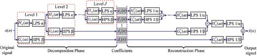
The analysis and synthesis filter banks for TQWT.
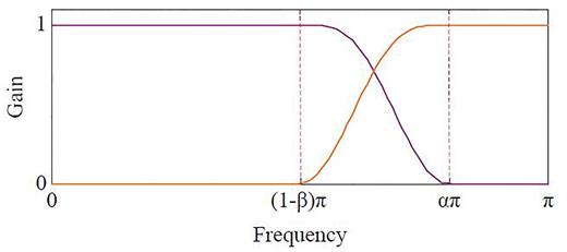
Frequency responses of the filters, H0(w) and G0(w).
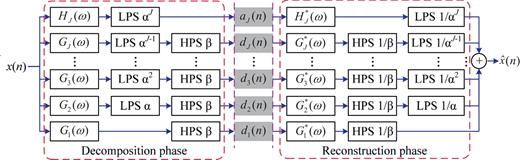
The equivalent system for the analysis and synthesis filter banks for TQWT.
Figs 4(a) and (c) are mother wavelet functions with Q = 1 and Q = 4, respectively. The role of the Q-factor can be easily observed from the shape of the wavelet. For the low Q-factor, the wavelet has fewer sign changes and consists of fewer oscillatory cycles. On the contrary, for the high Q-factor, the wavelet has more sign changes and consists of more oscillatory cycles. The corresponding frequency spectra are shown in Figs 4(b) and (d). It can be observed that the wavelet function with Q = 1, which is low-oscillatory in the time domain, shows a relatively wide bandwidth in the frequency domain. Contrarily, the wavelet function with Q = 4, which is high-oscillatory, exhibits a relatively narrow bandwidth. In a word, the oscillatory behaviour of the wavelet can be determined by adjusting the Q-factor of TQWT.
Wavelet functions with different Q-factors and their frequency spectra. (a) Wavelet function with Q = 1. (b) The frequency spectrum of wavelet function with Q = 1. (c) Wavelet function with Q = 4. (d) The frequency spectrum of wavelet function with Q = 4.
2.3 Optimal dictionary construction strategy
To illuminate the strategy of constructing the optimal dictionary, we employ the field shot gather, as shown in Fig. 5, which was collected from the Daqing oilfield in China, with 481 traces, a 10 m receiver interval, 6002 sampling points and a 1 ms sampling interval in the time direction. A nonlinear gain of 10 per cent is applied to clearly show the whole data field. We note that the ground-roll is very strong and spreads over a wide range, leading to unrecognizable seismic data, especially at near offsets.
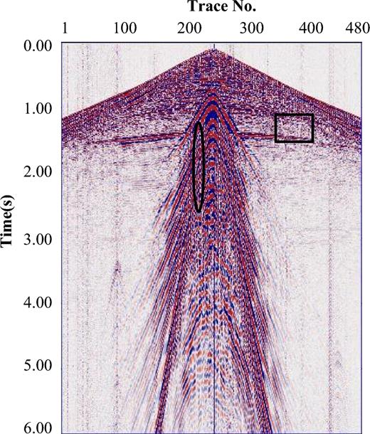
Field-shot gather of raw seismic data.
To construct the dictionaries, we need to first get the signal samples for each component. Although the ground-roll interferes with body waves in the real data, this work can be achieved by selecting specific traces and time windows that mainly contain one component. The far offset data, which is nearly unaffected by the ground-roll, is selected to extract body wave signals, and the near offset data, which is almost covered by the ground-roll energy, is chosen to extract ground-roll signals. For instance, signals in the rectangular and the elliptic regions shown in Fig. 5 are regarded as body wave and ground-roll samples, respectively. Because the raw seismic data is very complex, the average amplitude spectrum is used here to enhance the statistical property. In Fig. 6(a), the black solid line is the average amplitude spectrum for the body wave sample in the rectangular area, and the red dashed line is the corresponding envelope curve. Fig. 6(b) shows the average amplitude spectrum and the envelope curve for the ground-roll sample in the elliptic region. It can be observed that the body wave shows a relatively wide frequency bandwidth similar to that of the wavelet function with low Q-factors, while the ground-roll presents a relatively narrow bandwidth similar to that of the wavelet function with a high Q-factor. Thus, the body wave is low-oscillatory and the ground-roll is high-oscillatory.
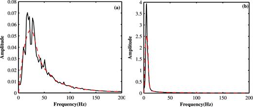
Average amplitude spectra of the body waves and ground-roll. (a) Average amplitude spectrum of the body waves in the rectangular region. (b) Average amplitude spectrum of the ground-roll in the elliptic region.
Based on the above analysis, TQWTs with different Q values are chosen as representative dictionaries for signal components with different oscillatory behaviours. By adjusting the Q-factor, oscillatory behaviour of the wavelet function can be determined to match the oscillatory behaviour of the signal component of interest; in this way, a sparse signal representation can be obtained. The more similar the signal component and wavelet function are, the better sparsity it shows. It should have a relatively low Q-factor to process low-oscillatory body waves. Nevertheless, a relatively high Q-factor is optimal when processing oscillatory ground-roll. In this study, the Q-factor of dictionary is empirically determined. To evaluate whether the constructed dictionary meets the key requirements for the MCA method, we measure the sparsity with L1-norm by the iterative shrinkage-threshold algorithm (Figueiredo & Nowak 2003; Daubechies et al. 2004), which is applied in subsequent synthetic and field data processing. Wavelet coefficients |$\boldsymbol{x}_1$| and |$\boldsymbol{x}_2$| are calculated iteratively until the computed result shows little change.
2.4 The morphology of the primary wave
To successfully apply the proposed method in the seismic field, distinguishable morphologies between the primary wave and ground-roll are essential. Herein, the morphology of the primary wave is illustrated. A primary reflection event on a seismic record is often considered to be the result of a process in which a down-going signal travels with weak dispersion to a geologic interface, reflects, and returns to the surface (Resnick et al. 1986). Because of its non-dispersive nature and high velocity, the primary wave is approximately linear and mainly distributed in a shallow position within the seismic data. Thus, the linear events in a shallow position of the field shot gather are selected to extract primary wave samples. For instance, linear events including traces from 440 to 460 in the shallow position of Fig. 5 are regarded as primary wave samples. Its average amplitude spectrum is shown in Fig. 7 as a black solid line, and the red dashed line is the corresponding envelope curve. It can be seen that the primary wave shows a relatively wide frequency bandwidth similar to that of the body waves in Fig. 6(a). Thus, the primary wave is low-oscillatory and separated together with the body waves. Therefore, the proposed method will do little damage to the primary wave.
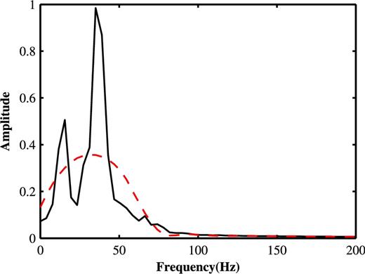
Average amplitude spectrum of the primary wave.
3 DATA EXAMPLES
In this section, the proposed method is applied to both synthetic and field seismic shot gathers. The performance and advantages of the proposed method are analysed and highlighted. Moreover, the high-pass filtering and f-k filtering schemes are used for comparison.
3.1 Synthetic data examples
In land shot gathers, the ground-roll has characteristics of high amplitude, low frequency and dispersive wave trains, as well as a low phase and group velocity. The body wave is simulated using the convolution model, while the ground-roll is created through 2-D time domain elastic finite difference modelling (Mills & Innanen 2017).
Fig. 8(a) shows the synthetic data containing two reflections. The effective reflections can be approximated by hyperbolas convoluted with the Ricker wavelet with a dominant frequency 40 Hz considering that the body wave is low-oscillatory. The synthetic shot superposed with the representative ground-roll is shown in Fig. 8(b), with 1250 traces, a 2 m receiver interval and 1000 sampling points and a 2 ms sampling interval in the time direction. The geologic models used for ground-roll modelling are shown in Fig. 9, with a width of 5000 m and a depth of 1500 m. An explosive point source using the Fuchs-Muller wavelet with a dominant frequency of 8 Hz is used to generate the ground-roll for radial and vertical components considering that the ground-roll is high-oscillatory, centred in the model (x = 2500 m, on the near surface discontinuity) at a depth of 5 m. Receivers are set every 2 m at a depth of 5 m. Furthermore, the boundary conditions apply free surface and the perfectly matched layer (PML) at other edges. Herein, the vertical component is used. Compared with Fig. 8(a), Fig. 8(b) shows typical wave trains from the ground-roll, which masks and distorts the reflections severely. And the primary wave here is very complex and different from real cases.
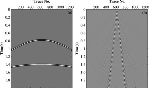
(a) Synthetic data containing two reflections. (b) Synthetic data superposed with ground-roll modelled through 2-D time domain elastic finite difference modelling.
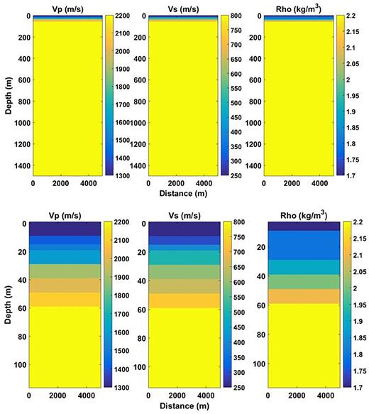
Geologic models used for synthetic modelling. Top: full model. Bottom: near surface zoom.
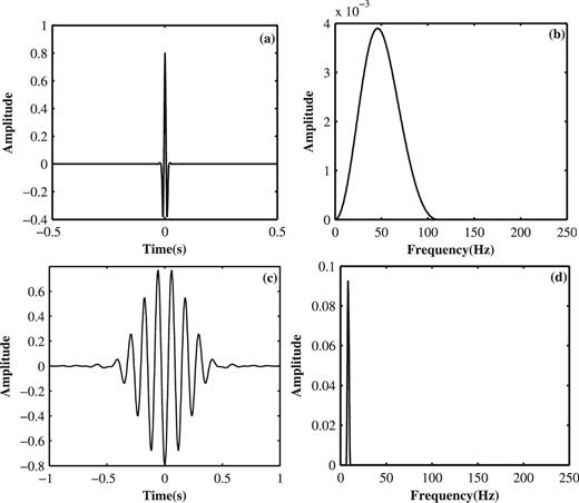
Fig. 10(a) shows the Ricker wavelet used in Fig. 8(a), with a dominant frequency of 40 Hz. Fig. 10(c) shows a section of the ground-roll component sample with the 760th trace from sampling points 201 to 1000 extracted from ground-roll modelling, as aforementioned. The frequency spectra for the body wave and the ground-roll are presented in Figs 10(b) and (d), respectively. Synthetic body waves exhibit a transient behaviour in the time domain and a relatively wide bandwidth in the frequency domain, while the ground-roll shows a sustained oscillation behaviour in the time domain and a relatively narrow bandwidth in the frequency domain. As can be seen, these two kinds of signals show different oscillatory behaviours and overlap with each other in the frequency range.
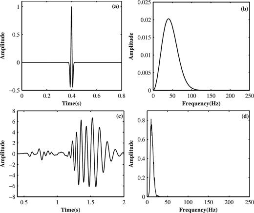
Waveforms of body wave and ground-roll in the time and frequency domains. (a) Ricker wavelet with a dominant frequency of 40 Hz used in simulating body waves. (b) Frequency spectrum of the body wave in (a). (c) Section of the ground-roll component sample with the 760th trace from sampling points 201 to 1000 extracted from ground-roll modelling. (d) The frequency spectrum of the ground-roll in (c).
In this data set, TQWTs with Q = 1 and Q = 4 are chosen as sparse representation dictionaries for body waves and the ground-roll by experience. The corresponding sparsity measurements using different dictionaries are shown in Table 1. The sparseness of TQWT with Q = 1 for body waves is about 5.72, while that for the ground-roll is about 9.95. The sparseness of TQWT with Q = 4 for the ground-roll is approximately 5.99, while that for body waves is approximately 9.57. From the results, we conclude that TQWT with Q = 1 works well as a representation dictionary for body waves, and Q = 4, for the ground-roll.
The sparsity estimation using TQWTs with Q = 1 and Q = 4.
| Body waves | Ground-roll | |
|---|---|---|
| TQWT with Q = 1 | 5.72 | 9.95 |
| TQWT with Q = 4 | 9.57 | 5.99 |
| Body waves | Ground-roll | |
|---|---|---|
| TQWT with Q = 1 | 5.72 | 9.95 |
| TQWT with Q = 4 | 9.57 | 5.99 |
The sparsity estimation using TQWTs with Q = 1 and Q = 4.
| Body waves | Ground-roll | |
|---|---|---|
| TQWT with Q = 1 | 5.72 | 9.95 |
| TQWT with Q = 4 | 9.57 | 5.99 |
| Body waves | Ground-roll | |
|---|---|---|
| TQWT with Q = 1 | 5.72 | 9.95 |
| TQWT with Q = 4 | 9.57 | 5.99 |
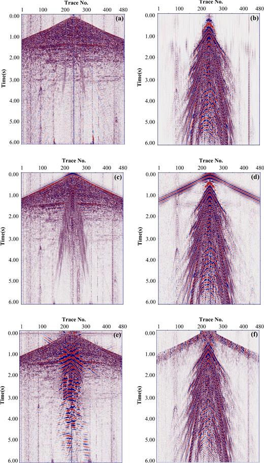
With the constructed dictionaries, the proposed method is applied to the synthetic data example. Figs 11(a) and (b) show the separated body waves and ground-roll, respectively. Comparing Fig. 11(a) with Fig. 8(a), we see that the noise is almost completely removed, and effective signals are fairly preserved at the mean time. Residual noise, which is low-oscillatory and kept as effective signal, can be attenuated by radon transform or f-k filtering on account of its linear regularity in the spatial direction. We see that the body wave component is almost invisible in Fig. 11(b), which indicates a tiny impairment of the effective signal. In order to make the effectiveness of the proposed method clearer, we use the results of both the high-pass and f-k filtering. High-pass filtering with a cut-off frequency of 15 Hz is applied to the synthetic data. Fig. 11(c) shows the obtained body waves, and the corresponding ground-roll shown in Fig. 11(d) is extracted by subtracting the filtered result from the original data. It can be seen that the high-pass filtering is effective at suppressing most of the ground-roll energy, however it weakens the low-frequency components of body waves. The body waves and ground-roll obtained by f-k filtering are presented in Figs 11(e) and (f). We can see that the f-k filter removes most of the ground-roll energy, discriminates the ground-roll cone accurately, and does little harm to signals outside this cone. However, the residual noise is distinct. A further comparison is shown in Fig. 12 by comparing the single trace results for the 760th trace of shot gather by these three techniques. Fig. 12(a) is the 760th trace of the composite signal extracted from Fig. 8(b). Fig. 12(b) is the simulated body waves with the 760th trace extracted from Fig. 8(a), while Fig. 12(c) is the simulated ground-roll. Figs 12(d) and (e) are the corresponding body waves and ground-roll components extracted from Figs 11(a) and (b). It can be observed that the results in Figs 12(d) and (e) are close to the simulated results in Figs 12(b) and (c), which means that the body waves and the ground-roll are almost completely separated. Likewise, Figs 12(f) and (g) are the 760th trace effective signal and separated ground-roll, corresponding to Figs 11(c) and (d), respectively. Figs 12(h) and (i) are the separated body waves and ground-roll, corresponding to Figs 11(e) and (f). It can be seen that by using high-pass and f-k filtering, obvious ground-roll residual exists in the separated body waves. The impairment for the low-frequency body waves is obvious in high-pass filtering. The f-k filter produces waveform distortions since the energy of the ground-roll is strong. From this comparison, we see that the proposed method is capable of separating signal components with different oscillatory behaviours, even when they have overlapping frequency bands. The proposed method exhibits better performance in preserving effective waveforms and suppressing the ground-roll. Moreover, it also shows the advantage of its high computational efficiency by the application of filter banks in the TQWT.
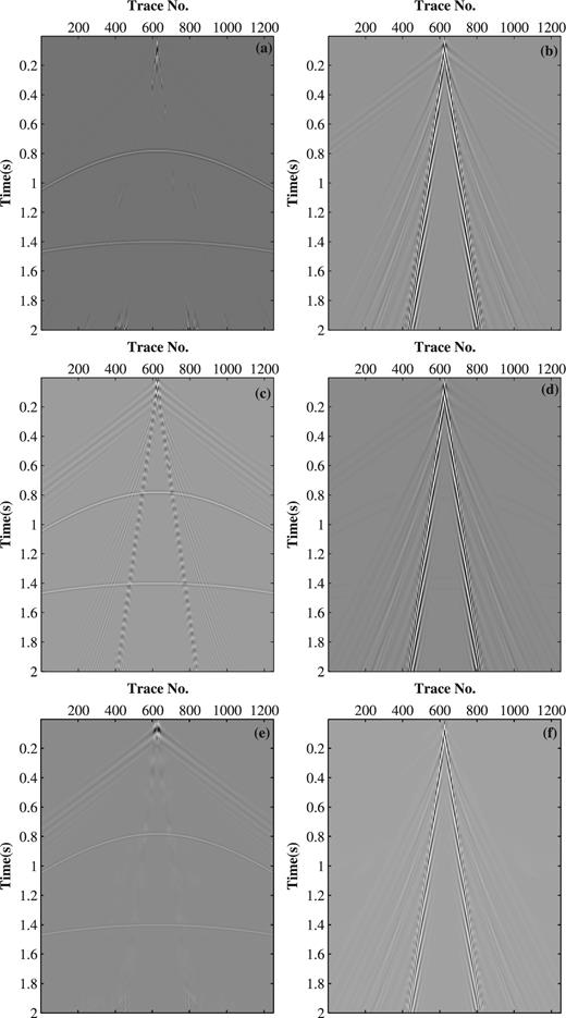
Comparison of the signal-noise separation results with multiple traces in the synthetic shot gather. (a) Body waves obtained using the proposed method. (b) Ground-roll obtained using the proposed method. (c) Body waves obtained using high-pass filtering. (d) Ground-roll obtained by subtracting the result of (c) from the raw data. (e) Body waves obtained using f-k filtering. (f) Ground-roll obtained by subtracting the result of (e) from the raw data.
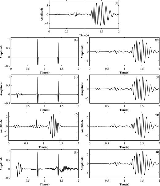
Comparison of the signal-noise separation results with the 760th trace in the synthetic shot gather. (a) Composite signal with the 760th trace. (b) Simulated body waves with the 760th trace. (c) Simulated ground-roll with the 760th trace. (d) Separated body waves with the 760th trace by the proposed method. (e) Separated ground-roll with the 760th trace by the proposed method. (f) Separated body waves with the 760th trace using high-pass filtering. (g) Separated ground-roll with the 760th trace using high-pass filtering. (h) Separated body waves with the 760th trace using f-k filtering. (i) Separated ground-roll with the 760th trace using f-k filtering.
3.2 Field data examples
To further examine the effectiveness of the proposed ground-roll suppression method, we apply it to the field shot gather shown in Fig. 5. For this shot gather, TQWTs with Q = 1 and Q = 3 are chosen as representation dictionaries for body waves and the ground-roll. The corresponding sparsity measurements of the signals in the rectangular and the elliptic regions using different dictionaries are shown in Table 2. The sparseness of TQWT with Q = 1 for body waves is about 8.10, while that for the ground-roll is about 8.86. The sparseness of TQWT with Q = 3 for the ground-roll is approximately 6.95, while that for body waves is approximately 9.41. It can be seen that TQWT with Q = 1 can represent body waves more sparsely, while TQWT with Q = 3 is better for the ground-roll. The estimated sparsity satisfies the key requirement for the MCA method.
The sparsity estimation using TQWTs with Q = 1 and Q = 3.
| Body waves | Ground-roll | |
|---|---|---|
| TQWT with Q = 1 | 8.10 | 8.86 |
| TQWT with Q = 3 | 9.41 | 6.95 |
| Body waves | Ground-roll | |
|---|---|---|
| TQWT with Q = 1 | 8.10 | 8.86 |
| TQWT with Q = 3 | 9.41 | 6.95 |
The sparsity estimation using TQWTs with Q = 1 and Q = 3.
| Body waves | Ground-roll | |
|---|---|---|
| TQWT with Q = 1 | 8.10 | 8.86 |
| TQWT with Q = 3 | 9.41 | 6.95 |
| Body waves | Ground-roll | |
|---|---|---|
| TQWT with Q = 1 | 8.10 | 8.86 |
| TQWT with Q = 3 | 9.41 | 6.95 |
Fig. 13(a) shows the obtained body waves by the proposed method, and Fig. 13(b) shows the extracted ground-roll. Further, both the high-pass filter and f-k filter were applied to the shot gather for comparison. The cut-off frequency of 8 Hz for the high-pass filter and rejected f-k regions for the f-k filter were both carefully chosen to achieve a compromise between reflection preservation and ground-roll suppression. Figs 13(c) and (d) show the separated body waves and ground-roll using high-pass filtering. Figs 13(e) and (f) show the corresponding results of f-k filtering. A further comparison is realized by intercepting data between 0 and 4000 ms. Figs 14(a)–(c) are the corresponding intercepted results from Figs 5, 13(a) and (b), respectively. Figs 14(d) and (e) are intercepted results from Figs 13(c) and (d), respectively. Figs 14(f) and (g) are for Figs 13(e) and (f). It can be seen that by using the proposed method, most effective events covered by strong ground-roll have been recovered, though a little primary wave loss can be observed. However, for high-pass filtering, ground-roll residual at near offsets is obvious, as shown in Fig. 14(d), and the loss of body waves can be observed around 1.5 s from Fig. 14(e). The f-k filter produces severe waveform distortions when processing the scattering ground-roll, as shown in Fig. 14(f). Primary wave loss can be seen at near offsets from Fig. 14(g). Moreover, a single trace data is chosen to further examine the effectiveness of this method. Fig. 15(a) shows the 252th trace of the raw seismic data in Fig. 14(a). Figs 15(b) and (c) show the 252th trace of the extracted body waves and ground-roll in Figs 14(b) and (c). Figs 15(d) and (e) are the body waves and ground-roll for the 252th trace in Figs 14(d) and (e), respectively. Figs 15(f) and (g) are the 252th trace body waves and ground-roll in Figs 14(f) and (g). Considering that the amplitude of the seismic waves in real data decays obviously with the spreading distance increased, signals in Fig. 15 are divided into two segments for a better and clearer comparison, that is, the 0–1000 ms section and the 500–4000 ms section. Moreover, the primary wave comparisons after ground-roll suppression by these three methods can be observed in the 0 to 1000 ms section. Figs 16(a) and (b) correspond to the two divided parts for Fig. 15(a). Similarly, Figs 16(c) and (d) correspond to Fig. 15(b), 16(e) and (f) correspond to Fig. 15(c), Figs 16(g) and (h) correspond to Fig. 15(d), Figs 16(i) and (j) correspond to Fig. 15(e), Figs 16(k) and (l) correspond to Fig. 15(f), and Figs 16(m) and (n) correspond to Fig. 15(g). We note that the proposed method does less harm to primary waves when it suppresses most of the ground-roll energy, whereas the high-pass and f-k filters damage the primary wave, as shown in the rectangular regions of Figs 16(i) and (m), and leave much ground-roll residual at near offsets, as shown in the rectangular regions of Figs 16(h) and (l).
Comparison of the signal-noise separation results with multiple traces in the field shot gather. (a) Separated body waves by the proposed method. (b) Separated ground-roll by the proposed method. (c) Extracted body waves using high-pass filtering. (d) Extracted ground-roll using high-pass filtering. (e) Extracted body waves using f-k filtering. (f) Extracted ground-roll using f-k filtering.
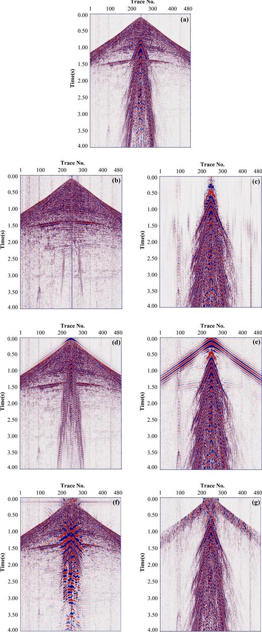
Intercepted results between 0 and 4000 ms of the field data. (a) Intercepted raw seismic data. (b) Intercepted body waves separated by the proposed method. (c) Intercepted ground-roll separated by the proposed method. (d) Intercepted body waves separated by high-pass filtering. (e) Intercepted ground-roll separated by high-pass filtering. (f) Intercepted body waves separated by f-k filtering. (g) Intercepted ground-roll separated by f-k filtering.
Comparison of the signal-noise separation results with a single trace between 0 and 4000 ms in the field shot gather. (a) The 252th trace waveform of the raw seismic data between 0 and 4000 ms. (b) Separated body waves by the proposed method. (c) Separated ground-roll by the proposed method. (d) Body waves using high-pass filtering. (e) Ground-roll using high-pass filtering. (f) Body waves using f-k filtering. (g) Ground-roll using f-k filtering.
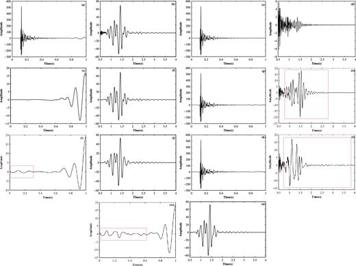
Data with 252th trace between 0 and 4000 ms are divided into two segments, that is, the 0–1000 ms section and the 500–4000 ms section (a) 0–1000 ms section of the raw seismic data. (b) 500–4000 ms section of the raw seismic data. (c) 0–1000 ms section of the body waves by the proposed method. (d) 500–4000 ms section of the body waves by the proposed method. (e) 0–1000 ms section of the ground-roll by the proposed method. (f) 500–4000 ms section of the ground-roll by the proposed method. (g) 0–1000 ms section of the body waves using high-pass filtering. (h) 500–4000 ms section of the body waves using high-pass filtering. (i) 0–1000 ms section of the ground-roll using high-pass filtering. (j) 500–4000 ms section of the ground-roll using high-pass filtering. (k) 0–1000 ms section of the body waves using f-k filtering. (l) 500–4000 ms section of the body waves using f-k filtering. (m) 0–1000 ms section of the ground-roll using f-k filtering. (n) 500–4000 ms section of the ground-roll using f-k filtering.
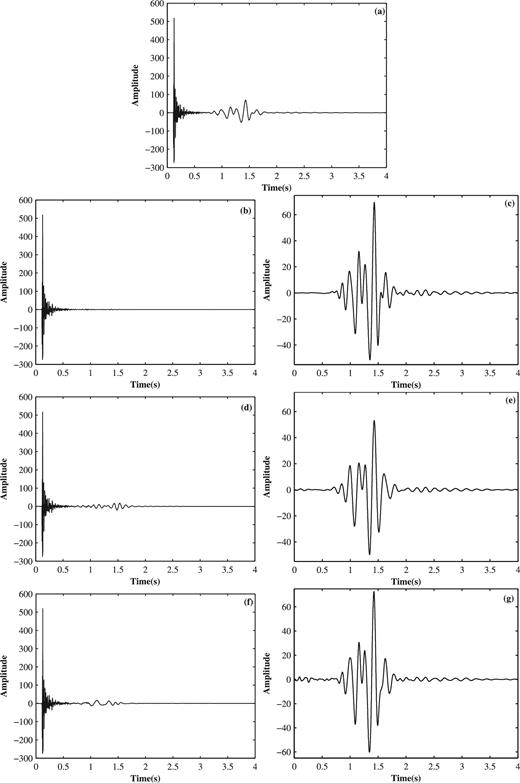
Furthermore, the real data after the brute stack will be shown as follows. The original data before the brute stack was collected from the Daqing oilfield including 20 shots, with 240 traces, a 20 m receiver interval and 2500 sampling points, and a 2 ms sampling interval in time direction for every shot. Herein, TQWTs with Q = 1 and Q = 3 are chosen as representation dictionaries for body waves and the ground-roll, respectively. Fig. 17(a) is the raw data with a 20-time brute stack. Fig. 17(b) shows the separated body waves by the proposed method after the brute stack. Fig. 17(c) shows the body waves by high-pass filtering with a cut-off frequency of 8 Hz after the brute stack. Fig. 17(d) shows the body waves by f-k filtering after the brute stack. It can be seen that the proposed method removes most of the ground-roll energy and maintains the lateral continuity of the reflections fairly well. The high-pass filter still has much ground-roll energy in the filtering result, and the f-k filter produces severe waveform distortions and destroys the lateral continuity of the reflections in the ground-roll affected areas. The average amplitude spectra of Fig. 17 are shown in Fig. 18. Fig. 18(a) is the average amplitude spectrum of the raw data after the brute stack. Fig. 18(b) shows the average amplitude spectrum of the real data after the brute stack, corresponding to the proposed method, and the high-pass and f-k filtering. It can be observed that the low-frequency information of the body waves is damaged severely by high-pass and f-k filtering.
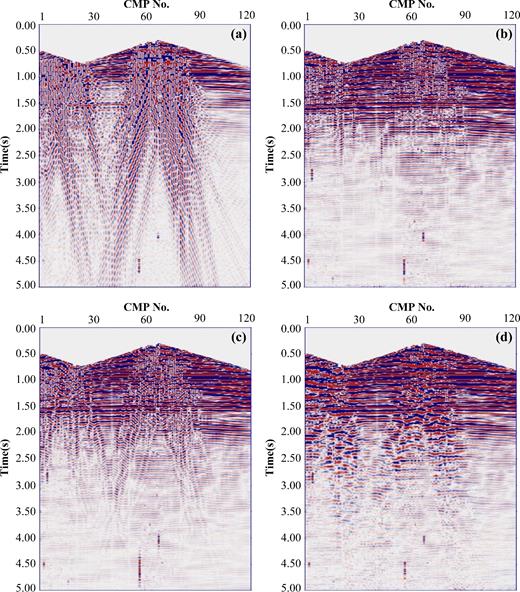
The real data after the brute stack, corresponding to the proposed method, high-pass filtering, and f-k filtering. (a) The raw data after the brute stack. (b) Separated body waves by the proposed method after the brute stack. (c) Separated body waves by high-pass filtering after the brute stack. (d) Separated body waves by f-k filtering after the brute stack.

The average amplitude spectra of the real data after the brute stack, corresponding to the proposed method, high-pass filtering, and f-k filtering. (a) The average amplitude spectrum of the raw data after the brute stack. (b) The average amplitude spectra of the separated body waves after the brute stack, corresponding to the proposed method, high-pass filtering, and f-k filtering.
Although the sparsity difference when processing the field data using the proposed method is not as obvious as that when processing the synthetic data, which is attributed to the interplay of body waves and ground-roll in the real seismic data, good separation results demonstrate that this sparsity-enabled method of constructing dictionaries is convenient and effective.
4 CONCLUSIONS
This paper presents a sparsity-enabled signal decomposition method for separating body waves and ground-roll. The main idea of the method is to construct dictionaries using TQWTs with different Q-factors in the MCA algorithm, owing to the different oscillatory behaviours of these two components. This method is implemented with an iterative procedure, which is very efficient and results in better preservation for the useful component after ground-roll suppression compared with conventional methods. Both synthetic and field-shot data are utilized to demonstrate the effectiveness of the presented method and its superiority over conventional high-pass and f-k filtering. Even though the proposed method is performed trace-by-trace, it effectively suppresses the scattering surface waves. While this study focuses its application on ground-roll attenuation, this method could also be extended to other applications to describe the oscillatory behaviours of different signal components. Future work is needed to construct the optimal dictionary to adaptively use TQWT.
Acknowledgements
The research was funded by the National Natural Science Foundation of China (41774135, 41504092 and 41504093), China Postdoctoral Science Foundation (2016T90925 and 2015M572567), the National Key Research and Development Program of China (2017YFB0202902), Fundamental Research Funds for the Central Universities and the Beijing Center for Mathematics and Information Interdisciplinary Science. We would like to thank the Exploration and Development Research Institute of Daqing Oilfield Company Ltd. for providing the data set. We also thank Dr. Yu Geng and Andrew Mills for their discussion and suggestions, and we are grateful to Dr. Baoli Wang for help in comparing results by conventional methods.
