


Summary
Surface waves propagating through sedimentary basins undergo elastic wavefield complications that include multiple scattering, amplification, the formation of secondary wave fronts and subsequent wave front healing. Unless these effects are accounted for accurately, they may introduce systematic bias to estimates of source characteristics, the inference of the anelastic structure of the Earth, and ground motion predictions for hazard assessment. Most studies of the effects of basins on surface waves have centred on waves inside the basins. In contrast, the purpose of this paper is to investigate wavefield effects downstream from sedimentary basins, with particular emphasis on continental basins and propagation paths, elastic structural heterogeneity and Rayleigh waves at 10 s period. Based on wavefield simulations through a recent 3-D crustal and upper-mantle model of East Asia, we demonstrate significant Rayleigh wave amplification downstream from sedimentary basins in eastern China such that Ms measurements made on the simulated wavefield vary by more than a magnitude unit. We show that surface wave amplification caused by basins results predominantly from elastic focusing and that amplification effects produced through 3-D basin models are reproduced using 2-D membrane wave simulations through an appropriately defined phase velocity map. The principal characteristics of elastic focusing in both 2-D and 3-D simulations include (1) retardation of the wave front inside the basins; (2) deflection of the wave propagation direction; (3) formation of a high-amplitude lineation directly downstream from the basin bracketed by two low-amplitude zones and (4) formation of a secondary wave front. We illustrate with several examples how the size and geometry of the basin affects focusing. Finally, by comparing the impact of elastic focusing with anelastic attenuation, we argue that on-continent sedimentary basins are expected to affect surface wave amplitudes more strongly through elastic focusing than through the anelastic attenuation except near the edge of the basin or for basins with extreme aspect ratios.
1 INTRODUCTION
The Earth's interior is heterogeneous in composition and phase. This is particularly true near the Earth's surface, where the presence or absence of sedimentary basins is a principal contributor to lateral heterogeneity in the shallow Earth. However, because sedimentary basins amplify seismic noise, seismologists tend to site seismic stations outside of basins. Together with the fact that earthquakes commonly occur either deep within basins or below them, this means that seismic body waves are often recorded with a minimal imprint of the effect of basins. As a result, sedimentary basins are often poorly modeled (e.g. Xie et al.2017) and this makes it more difficult to recover information about structures below them than in regions devoid of basins (e.g. Ferreira et al.2010).
These considerations are not true for surface waves, which are trapped near Earth's surface and propagate through sedimentary basins even to stations that may be situated outside of them. Thus, surface waves hold key information about sedimentary basins and are affected by them strongly. There have been many studies of the effects of sedimentary basins on the amplification of surface waves that are recorded within a basin (e.g. Aki & Larner 1970; Bard & Bouchon 1980a,b; Bard et al.1988; Olsen et al.1995, 2006, 2009; Kawase 1996; Alex & Olsen 1998; Olsen 2000; Graves et al.2011; Day et al.2012; Denolle et al.2014; Bowden & Tsai 2017). These studies interpret such amplitude effects as a ‘site response’ of the basin, which is seen to terminate at the boundary of the basin. The physical cause of the site amplification inside basins is predominantly constructive interference between body and surface waves (e.g. Kawase 1996), which is commonly regarded as a 2-D vertical cross-section effect. In comparison, there are very few studies of the residual effects on surface waves after they have passed through a basin. This is particularly true regarding the role of lateral heterogeneity on the surface waveforms at short to intermediate periods that propagate over regional distances, although surface wave focusing/defocusing caused by lateral heterogeneity has been studied at intermediate to long periods for waves that propagate over teleseismic distances (e.g. Lay & Kanamori 1985; Woodhouse & Wong 1986; Wang et al.1993; Wang & Dahlen 1995; Selby & Woodhouse 2000; Yang & Forsyth 2006).
The purpose of this paper is to attempt to improve understanding of the nature of elastic propagation effects on surface waves, particularly their amplitudes downstream from sedimentary basins. The focus of the paper is on lateral wavefield effects on Rayleigh waves at 10 s period, which is typically well excited by small earthquakes and nuclear explosions and is also well represented in ambient noise cross-correlations that are commonly used in tomographic studies (e.g. Shapiro et al.2005; Yang et al.2007; Lin et al.2009; Shen et al.2013a,b; Kang et al.2016; Shen & Ritzwoller 2016). The existence and nature of sedimentary basins strongly affect regionally propagating Rayleigh waves at this period. To the best of our knowledge, the work we present here is the first systematic study of the basin residual effects on short-period through-passing surface waves. As discussed below, our results indicate that a significant fraction of the observed amplitude variability is caused by 2-D elastic focusing/defocusing due to lateral wave propagation effects. The amplitude anomalies caused by 2-D focusing/defocusing can be significantly larger than site amplification inside basins as well as anelastic attenuation.
We mention now two examples how this paper large is relevant to other studies.
The inference of the anelastic structure of the Earth based on surface wave amplitude information may be biased by amplitude effects caused by elastic structures. Some studies of surface wave attenuation have taken focusing/defocusing into account (e.g. Dalton & Ekstrom 2006; Dalton et al.2008; Bao et al.2016), but have applied corrections only at long periods. At shorter periods, surface wave attenuation tomography has been performed by extracting amplitude information from ambient noise (e.g. Prieto et al.2009; Lawrence & Prieto 2011). Such studies typically assume, however, that focusing and defocusing average out in the data processing. Ignoring elastic focusing effects can produce locally negative values of effective Q which are actually commonly observed but are often discarded in observational studies (e.g. Levshin et al.2010).
Source characterization generally, and moment or magnitude estimation specifically, depend in part on interpreting the amplitude of surface waves that propagate at regional distances. Strong amplitude effects imparted to surface waves by elastic heterogeneities may bias magnitude estimates and other source characteristics. This may be particularly important in the context of nuclear discrimination. Indeed, the ability to discriminate nuclear explosions from naturally occurring seismic events such as earthquakes rests in part on the ability to measure reliably and interpret the amplitude of body and surface waves that are generated by these sources. Body and surface wave amplitude measurements are commonly converted into the magnitude estimates mb and Ms, respectively. Although many nuclear explosions are characterized by a large mb: Ms ratio relative to most earthquakes, there are exceptions (e.g. Bowers & Selby 2009; Selby et al.2012). Strong spatial variations in the amplitudes of surface wave have been observed for nuclear tests in North Korea (e.g. Bonner et al.2008; Koper et al.2008; Zhao et al.2008; Shin et al.2010). Fig. 1 presents five Ms measurements observed with real data following a North Korean nuclear test in 2006 to illustrate the variation of observed Ms (measurements are obtained from Pasyanos, private communication, 2017). It also shows Ms predictions from a numerical simulation through a recent 3-D model (Shen et al.2016). We describe the details of the numerical simulations in Sections2–4. Both the real data and the predictions show a similar pattern of amplification and de-amplification in Ms. One of the principal goals of this paper is to illuminate the physical cause of such amplifications effects.
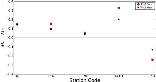
Illustration of the variations of Ms measurements using real data (red dots, 2006 DPRK nuclear test) compared with Ms predictions based on the China Reference Model (black dots). The measurements are provided by Pasyanos (private communication, 2017), obtained at the stations indicated on the horizontal axis. The data shown are differences relative to the average Ms of each data set, which is 3.1 for the real data and 3.15 for the numerical predictions.
The paper is organized in three parts. The first part of the paper illustrates the importance of the impact of elastic heterogeneity on through-passing short-period surface waves. This comprises Sections 2–4, where we present a 3-D wavefield simulation in East Asia (Fig. 2), a region chosen because of the presence of significant sedimentary basins, identified by cross-hatching in Fig. 2 and named in Table 1. We describe the Earth model used in the 3-D simulations and the corresponding numerical schemes (Section 2) and present simulated observations of surface wave traveltimes and amplitudes (Section 3) across East Asia at 10 s period. The final section of the first part illustrates how elastic structure would bias surface wave magnitude (Ms) measurements when the amplitude effects of elastic heterogeneity are ignored. The 3-D wavefield simulations across East Asia are based on the code SES3D, which is a 3-D spectral-element solver in spherical coordinates (Gokhberg & Fichtner 2016). One of the features of this code is that it is straightforward to implement arbitrary 3-D models.
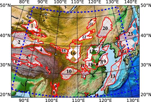
The blue dashed box encloses the study region in which stippled areas identify the sedimentary basins, which are named in Table 1. The red star is the location of the source for the 3-D simulation near the North Korea nuclear test site.
Major basins in the study region. Numbers are found in Fig. 2.
| Zones | Major basins |
|---|---|
| Xiyu (Northwestern China) | Junggar Basin (1) |
| Tarim Basin (2) | |
| Turpan Basin (3) | |
| Tibetan Plateau and Nearby | Qaidam Basin(4) |
| Areas | Qiangtang Tanggula Basin (5) |
| Cuoqing Lunpola Basin (6) | |
| Qabdu Basin (7) | |
| Chuxiong Basin (8) | |
| Southeastern Tibet | Lanping-Simao Basin (9) |
| South China | Sichuan Basin (10) |
| Nanyang Basin (11) | |
| Jianghan Basin (12) | |
| East China Sea Basin (13) | |
| Pearl River Mouth Basin (14) | |
| North China Craton and Nearby | Jiuquan Minle Wuwei Basin (15) |
| Seas | Ordos Basin (16) |
| Bohaiwan Basin (17) | |
| Taikang Hefei Basin (18) | |
| Subei Yellow Sea Basin (19) | |
| Northeastern China, Korean | Songliao Basin (20) |
| Peninsula and the Sea of Japan | Temtsag Hailar Basin (21) |
| Erlian Basin (22) | |
| Sea of Japan Backarc Basin (23) | |
| Tsushima Basin (24) |
The second part of the paper comprises Section 5, which aims to illuminate the physical cause(s) of the surface wave amplitude anomalies across East Asia simulated in the first part of the paper. The full-waveform numerical examples presented in this part of the paper are carried out using SPECFEM2D (e.g. Komatitch et al.2001) and SW4 (Petersson & Sjogreen 2014), which are designed for 2-D and 3-D wavefield simulations in Cartesian coordinates, respectively. We propose that 2-D lateral elastic focusing is the dominant physical cause of amplitude anomalies for short-period surface waves propagating in a 3-D Earth. This lateral focusing effect includes several principal characteristics that can be observed in both 2-D and 3-D simulations, which are: (1) retardation of the wave front inside the basin; (2) deflection of the wave propagation direction; (3) a high-amplitude lineation or stripe directly downstream from the basin bracketed by two low-amplitude zones and (4) formation of a secondary wave front. We also quantitatively show that most of the wavefield effects observed in the 3-D simulations can be reproduced quite accurately with horizontal 2-D membrane wave simulations.
Section 6 is the third part of the paper in which we discuss how surface wave focusing depends on the scale and geometry of the basin and compare the effects of anelastic attenuation with elastic focusing. We show that on a regional scale elastic focusing through sedimentary basins is more likely to cause significant surface wave amplitude anomalies than anelastic attenuation produced by the basins.
2 NUMERICAL SCHEMES FOR THE SIMULATION ACROSS EAST ASIA
We describe here the numerical setups for the 3-D simulation across East Asia, which include descriptions of the input 3-D velocity model, the Q model, surface topography, the source parameters and the numerical mesh. The simulation code is SES3D, a 3-D seismic wave equation solver based on the spectral-element method (Gokhberg & Fichtner 2016). The 3-D model is a recent model of the crust and uppermost mantle constructed for China by Shen et al. (2016).
2.1 3-D velocity model
The input Earth model for the full-waveform simulation is a recently produced 3-D isotropic model of the crust and uppermost mantle beneath China (Shen et al.2016) developed using Rayleigh wave dispersion measurements (8–50 s period) obtained from ambient noise and earthquake tomography. The model is intended as a reference for studies like ours, and the authors refer to it as a ‘China Reference Model’. The model is presented on a 0.5° × 0.5° grid and extends from the surface to a depth of 150 km. The authors of the model took care in representing sedimentary basins in which sedimentary structure is summarized with three unknowns at each grid node: sedimentary thickness and the top and bottom shear wave speeds (Vs) in the basin. Vs grows monotonically and linearly with depth in the sediments. The densities of the sediments and the crystalline crust are computed from Vs using the scaling relationship of Brocher (2005), whereas Vp/Vs is 2.0 in the sediments and 1.79 in the crystalline crust.
The geographical region of the model is shown in Fig. 2 by the blue box near whose boundary we place a perfectly matched layer (PML, Berenger 1994). Similarly, there is a PML at 200 km depth. Because the simulation code, SES3D, does not model seismic wave propagation in water, we replace water layers with sediments, but we design the sedimentary structure at each location to fit the observed local surface wave speeds from the study of Shen et al. (2016). The largest impact of this replacement occurs in the Sea of Japan, where water depth is the greatest. Because this results in a physically unrealistic model off the coast, we attempt to confine our simulation to the continent as much as possible. The original China Reference Model has an irregular shape; therefore, we smoothly extrapolate the edges of the original model to get a ‘rectangular’ model that is acceptable for our simulations.
Fig. 3 illustrates some of the structural features of the China Reference Model by presenting horizontal slices of Vs at the depths of 3, 10 and 20 km as well as topography on the Moho. The model captures many geological structures of the uppermost crust such as the Songliao Basin, the Bohaiwan Basin, the Sichuan Basin and the Subei Yellow Sea Basin, which are all seen on the 3 km depth slice.

The 3-D model is an oversimplification of sedimentary structure, although it fits surface wave phase speeds quite well across our study region. Shen et al. (2016) show that the standard deviation of the misfit to interstation phase time measurements is less than 1 s at most periods. As is common with tomographic models, the amplitude and sharpness of the structural anomalies are probably underestimated, a problem that grows in significance as structures reduce in spatial size. We believe, however, that the model is the best alternative to represent structural effects on surface waves across the study region.
2.2 Q model
For anelasticity, we replace the 3-D Q model employed by Shen et al. (2016) with the 1-D Q model of Durek &Ekström (1996) because we are primarily interested in the impact of lateral variations in elastic structures on surface waveforms. The viscoelastic relationship is implemented in the simulation using a series of Standard Linear Solids (SLS). We find a set of relaxation times and the corresponding weights using a simulated annealing algorithm (Kirkpatrick et al.1983), which results in an almost constant Q from about 10–20 s period. The result of using a 1-D Q model is that all lateral variations in the wavefield will derive exclusively from elastic structure.
2.3 Surface topography
Surface topography is not implemented in the simulation because our interest centres on the impact of elastic velocity heterogeneity within the Earth on short-period surface waves. This is also due to the fact that the effect of topography on the 10 s surface waves is believed to be negligible (e.g. Kohler et al.2012).
2.4 Source parameters
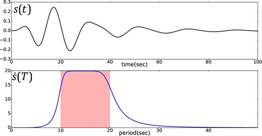
Source time function. The upper panel is the time-series, while the lower one is the time derivative of the source time function in the period domain. (Far-field displacement is proportional to the derivative of the source time function).
2.5 Mesh setup
Our study focuses on the analysis of the 10 s Rayleigh wave, which can be accurately simulated with a mesh scheme in which the maximum element size is around 6 km. Because each element has five cells with nodes located at the Gauss–Lobatto–Legendre points, the maximum grid spacing is approximately 1.2 km. Because the minimum wavelength in the simulation is 10 km (minimum shear wave velocity is 1 km s−1 in the model), 8.3 gridpoints per minimum wavelength is sufficient for our simulation (larger than the five gridpoints per minimum wavelength suggested by Komatitsch & Tromp 1999, for example).
3 WAVEFIELD ANALYSIS
Vertical component wavefield snapshots at times of 120, 460, 700 and 1020 s after the initiation of the source are presented in Fig. 5. The Rayleigh wave dominates these wavefields. A corresponding wavefield animation can be found in the Supporting Information. Wave front distortions are primarily caused by the sedimentary basins. There are four principal types of distortion. (1) The wave front is retarded and buckles inward during propagation through a basin (e.g. 460 s snapshot, Fig. 5b). (2) The wavefield propagation direction is deflected. (3) After the wave front emerges from a basin it amplifies, and there is attendant de-amplification that brackets the region of strong amplification. (4) The basins generate a secondary wave front with a smaller radius of curvature that trails the primary wave front (e.g. 700 s inset, Fig 5c). Note that the de-amplification is harder to observe in the 3-D wavefield simulation through the China Reference Model, but we attempt to clarify it in the simulations through idealized structures presented later in the paper. The basin that has the largest impact on the wavefield is the Bohaiwan Basin.
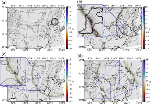
Wavefield snapshots at times t = 120, 460, 700 and 1020 s. (a) At t = 120 s, the wave front is still approximately circular. (b) At t = 460 s, the wave front is traveling through the Bohaiwan and Subei basins and has been greatly distorted. (c) At t = 700 s, a secondary wave front has been generated where amplification occurs, shown in the inset. (d) At t = 1020 s, the Sichuan basin's impact on the wave front is apparent.
Given the synthetic seismograms from the simulation, we measure the dispersion curves for phase velocity and spectral amplitudes to determine the traveltime (Fig. 6a) and amplitude maps (Fig. 6b). We make these measurements using frequency–time analysis (FTAN, Levshin et al.1972; Levshin & Ritzwoller 2001). Although the simulation is for the band between 10 and 20 s period, we concentrate interpretation at 10 s period because the impact from sedimentary basins is stronger at the shorter period end of our bandwidth of study. Large amplitude stripes appear (Fig. 6b) where the traveltime level lines cave inward (Fig. 6a).
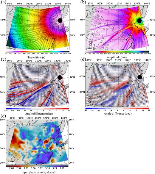
Plots of 10 s Rayleigh wave measurements in the 3-D simulation through the China Reference Model of (a) traveltime, (b) amplitude and (c) angular difference between the propagation direction and the local great circle direction. (The angle is defined in polar coordinates with the axis pointing to the East, counterclockwise direction is positive.) (d) Angular difference between 2-D ray tracing propagation direction and the local great circle direction. (e) Input phase velocity map (10 s Rayleigh wave) for the ray tracing computation in (d).
For comparison, we also present in Fig. 6(d) the direction of propagation and deviation from the great circle path using traveltimes computed by 2-D ray tracing on a sphere followed by the application of the eikonal equation. This is computed using the phase speed map in Fig. 6(e) from the China Reference Model. Ray tracing is performed with the fast-marching method of Rawlinson & Sambridge (2004) for the 10 s Rayleigh wave. We also discuss this result in Section 5.
4 BIAS OF SURFACE WAVE MAGNITUDES DUE TO ELASTIC PROPAGATION EFFECTS
As discussed earlier, reliable surface wave magnitude (Ms) measurements are needed to help discriminate nuclear explosions from earthquakes because many explosions are characterized by a large mb: Ms ratio relative to most earthquakes (e.g. Bonner et al.2008; Bowers & Selby 2009). Here, we illustrate how large of a bias can be introduced in the Ms measurement unless 3-D propagation effects through sedimentary basins are taken into account.
Fig. 7 presents the resulting Ms measurements through the China Reference Model at 10 s period, which vary from 2.5 to 3.9 across the study region. The range of variation is similar to measurements made on real data across the region (e.g. Pasyanos, private communication, 2017), a subset of which are shown in Fig. 1. The five Ms measurements from real data (2006 DPRK Nuclear Test) shown in Fig. 1 are presented with triangles in Fig. 7. The colour inside the triangles indicates the Ms measurement from real data. We discarded Ms estimates from stations that have an epicentral distance Δ < 500 km, which may suffer from near-field complications of the wavefield. The five real Ms measurements indeed show amplification and de-amplification in accord with predictions. Further data analysis, which is beyond the scope of this paper, is called for in the future to investigate this comparison further.
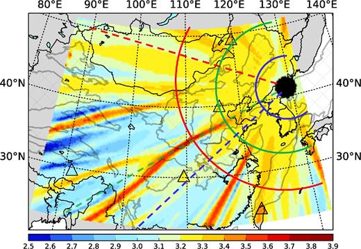
Surface wave (Ms) map (10 s), computed using Russell's formula (Russell 2006) from the amplitude map (Fig. 6b) taken from the 3-D simulation through the China Reference Model. The colour of the triangles indicates Ms measurements extracted from real data (2006 DPRK Nuclear Test, Pasyanos, private communication, 2017). For comparison, as in Fig. 1, the mean of the measurements has been shifted to the mean of the predictions. The coloured solid and dashed lines mark locations for the azimuthal- and distance-dependent curves shown in Fig. 8.
Because the reference Ms = 3.2, we consider Ms estimates that fall in the range from 3.1 to 3.3 as unaffected by elastic amplification or de-amplification. More than one-third of the region has measurements that are biased outside this range. The Ms map clearly illustrates attendant de-amplification zones that bracket the stripes of strong amplification. We discuss this effect further in Section 5.
Fig. 8 illustrates the variation of measurements of surface wave amplitude and Ms with azimuth and distance. The selected grid nodes for Fig. 8 are identified with bold colour-coded lines in Fig. 7. Assessment of azimuth variation is based on three groups of grid nodes at different distances (distance ∼500, 1100 and 1700 km) and is shown in Figs 8(a) and (c). For a distance of about 500 km (blue dots), amplitude measurements display very little azimuthal variation and Ms estimates are approximately constant. However, for a distance of about 1100 km (green dots), the measurements oscillate with azimuth and display several peaks or troughs due to amplification and de-amplification. At greater distances (∼1700 km, red dots), the peaks corresponding to the amplifications become narrower with larger variations in both amplitude and Ms. To illustrate the variation with distance, we also group our measurements in three azimuth ranges in Figs 8(b) and (d) at azimuths of 235°–236° (blue dots), 253°–254° (green dots) and 300°–301° (red dots), respectively. The 253°–254° azimuth range has the largest amplification effect, while the 235°–236° range is expected to be de-amplified as it is between two amplification stripes. The 300°–301° range has neither amplification nor de-amplification. Two of these groups of measurements (235°–236° and 300°–301°) display a clear decay of amplitudes with distance, while for the de-amplification azimuth range (235°–236°) amplitudes tend to be systematically smaller than the other groups at distances larger than 1500 km. The Ms measurements in the anomalous two groups of measurements (235°–236°, 253°–254°) shown in Fig. 8 illustrate how Russell's empirical formula does not account for the amplitude variation in a 3-D Earth model.
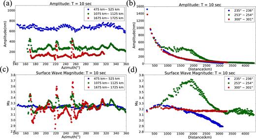
Detailed plots of the 10 s Rayleigh wave amplitude and Ms as a function of distance and azimuth from the 3-D wavefield simulation through the China Reference Model. Locations of the points on these plots are presented in Fig. 7 where those lines are coloured coded as the symbols in this figure. (a) and (b) are the amplitude measurements, while (c) and (d) are the Ms estimates. The full amplitude field across the study region is shown in Fig. 6(b) and the Ms across the region is shown in Fig. 7. Ms ∼ 3.2 for a laterally homogeneous model.
In summary, elastic structures in sedimentary basins strongly impact both surface wave amplitudes and Ms estimates of regionally propagating surface waves at 10 s period. Amplitudes may be several times larger and the Ms variation can be as large as 1.4 magnitude units across East Asia for events on the North Korea nuclear test site.
5 THE PHYSICAL CAUSE OF SURFACE WAVE AMPLIFICATION/DE-AMPLIFICATION—2-D LATERAL FOCUSING/DEFOCUSING
In this section, we propose a physical mechanism to explain the amplitude effect that we observe in the 3-D simulation. If we take a closer look at the wavefield snapshot (t = 730 s) shown in Fig. 5(c), large amplification occurs where the wave front travels through the Bohaiwan Basin. We also note that a secondary wave front (a wave front with larger curvature compared with the major one) is generated at the amplification location. Because of this, we hypothesize that the amplitude anomalies observed from the 3-D simulation across East Asia are predominantly caused by 2-D focusing due to lateral heterogeneity, rather than more complicated 3-D effects that may include vertical scattering and mode mixing.
5.1 2-D focusing effect
The 2-D focusing effect proposed here is fundamentally a wave front deflection phenomenon due to the impact of a lateral velocity heterogeneity. Fig. 9 illustrates the principal characteristics of the 2-D focusing effect, depicting the effect of a low-velocity anomaly on a surface wavefield. When the wave front propagates through the anomaly, we would observe:
The formation of a wavefield concavity inside the velocity anomaly.
The deflection of wave propagation direction, which indicates the bending of the wavefield energy flux.
A high-amplitude lineation or stripe directly downstream of the anomaly bracketed by two low-amplitude zones. This is due to the fact that the wavefield energy off centre-axis flows into the centre and is fundamentally a consequence of conservation of energy.
A secondary wave front with a smaller radius of curvature than the primary wave front outside the velocity anomaly, which is radiated from the focal point where the energy converges.
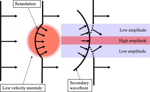
Cartoon summarizing some of the principal wave front characteristics in our 3-D simulations including the formation of a concavity inside the low-velocity anomaly, the formation of a secondary wave front with a smaller radius of curvature than the primary wave front, the bending of the primary wave front as it adheres to the secondary wave front (dashed lines) and amplification/de-amplification downstream from the velocity anomaly. Wave fronts are shown with solid lines and the normals to them are shown with arrows, which represent local wavefield propagation directions.
If true, these principal characteristics should be observed in both 2-D and 3-D wavefield simulations. Because we propose that 2-D focusing/defocusing dominates the amplitude effect downstream from sedimentary basins for surface waves propagating in a 3-D Earth, we also need to evaluate quantitatively the consistency between the 2-D and 3-D amplitude predictions. In the following sections, we verify these characteristics of the wavefield that are needed to support the hypothesis that 2-D focusing dominates the amplitude effect for surface waves propagating in a 3-D Earth.
5.2 Wave front bending and amplification
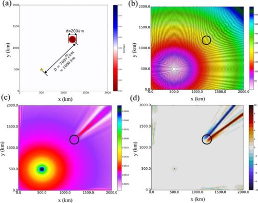
A 2-D membrane wave simulation to illustrate the impact of a low-velocity anomaly on the deflection of the propagation direction. (a) Input velocity model and source location, (b) traveltime map, (c) amplitude map, (d) angular difference between the propagation direction and the straight ray path. (The angle is defined in polar coordinates where the axis points to the right and the counterclockwise direction is positive). The impact of a 2-D low-velocity anomaly or ‘basin’ is to produce a high-amplitude streak downstream from the anomaly in (c) which is bracketed by two de-amplification stripes. The amplification stripe is also bracketed by lines of wavefield deflections clockwise (blue) and counterclockwise (red) in (d). This signature of wavefield amplification/de-amplification and deflection is characteristic of surface wave focusing and is also seen in the 3-D wavefield simulation (e.g. Figs 6b and c).
These principal characteristics (1)–(3) of 2-D focusing are also observed in the 3-D simulation across East Asia. Indeed, Fig. 6(a) shows the distortion of the traveltime contour when the wavefield propagates through the Bohaiwan Basin, and the location of the distortion is consistent with the largest amplification stripe in the amplitude map (Fig. 6b). As mentioned earlier, the attendant low-amplitude zones that bracket the amplification stripe can be identified in Fig. 7. Also, the propagation deflection map (Fig. 6c) computed by using the eikonal equation indicates that all the amplification stripes that emerge in the amplitude map (Fig. 6b) are caused by bending and focusing of the energy flux of the wavefield.
For a simple comparison, Fig. 6(d) shows the ray tracing result computed using the input phase velocity map presented in Fig. 6(e). The full-waveform propagation deflection map (Fig. 6c) has more detailed bifurcations and somewhat larger magnitudes of the off-great circle deflection than the ray theoretical propagation deflection map (Fig. 6d), which may be due to wavefield scattering.
5.3 2-D versus 3-D amplitude predictions
Another piece of evidence we need to provide to support the hypothesis that 2-D focusing dominates the amplitude effect for surface waves propagating in the 3-D Earth is to quantitatively compare amplitude predictions generated by 2-D and 3-D simulations.
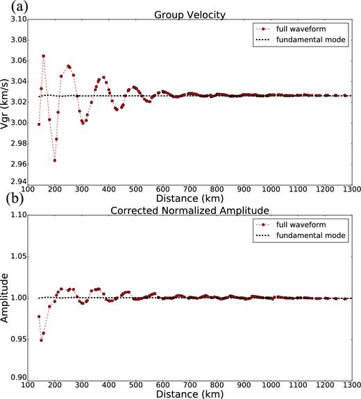
Synthetic experiment at 10 s period to test overtone interference on measurements of the fundamental mode in a 3-D simulation. Red dots result from a 3-D simulation through a laterally homogeneous model, whereas the black dashed lines represent fundamental mode synthetic results through the same model. (a) Measured group velocity and (b) corrected normalized amplitude measurements are presented as a function of epicentral distance. Oscillations in the measurements made on the 3-D synthetics are caused by overtone interference near the source where the overtones and fundamental mode are not yet separated in time. Amplitude interference decays below about 1 per cent at distances beyond 200 km, whereas group velocity perturbations extend to greater distances.
We conclude that for 10 s period and source–receiver distances greater than about 200 km, overtone interference is weak enough to interpret amplitude measurements made on the fundamental mode. Only at epicentral distances greater than 200 km, therefore, can we compare amplitude measurements obtained on 2-D and 3-D synthetics.
Fig. 12 illustrates the input models for the comparison between the 2-D and 3-D simulations. The input model for the 3-D simulation is a rectangular region with dimensions 5000 km × 600 km × 200 km (the green rectangle in Fig. 12b), in which an explosive source is located at x = 500 km, y = 300 km and z = 1 km. The velocity structure is ak135 in which a circular sedimentary basin is embedded centred at x = 1500 km and y = 300 km. The basin has a diameter of 200 km and extends to a depth of 5 km. Shear wave velocity inside the basin increases linearly with depth from 2 km s−1 at the top (z = 0 km) to 3 km s−1 at the bottom (z = 5 km) of the basin. Fig. 12(a) illustrates the 3-D shear wave speed profiles inside and outside the basin.
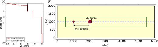
Specification of the input 2-D and 3-D models to test the similarity of wavefield measurements obtained in 2-D and 3-D simulations. (a) Vertical Vs profile for the 3-D input model (red line with dots: inside the basin and black line: outside the basin). (b) Input model geometry for the simulations. The green rectangle is the size of 3-D simulation region, whereas the black rectangle is the 2-D simulation region. The red star is the location of the source. Receivers are aligned on the horizontal blue dashed line.
The 2-D model is constructed from the 3-D model. In fact, the 2-D phase velocity map for the 10 s Rayleigh wave is the input model for the 2-D membrane wave simulation. Because the absorbing boundary conditions (Stacey 1988) implemented in the 2-D membrane wave code (SPECFEM2D) do not perform ideally and artificial reflections from the boundaries are generated, the 2-D simulation region is larger than the 3-D case. As shown in Fig. 12(b), the green rectangle represents the size of the 3-D simulation region, while the black one illustrates the size of the 2-D modeling region.
Fig. 13 presents wavefield snapshots from the 3-D and 2-D simulations. The principal difference is that the wavefield in 2-D is non-dispersive, whereas the wave front in 3-D is dispersed, and is therefore wider. However, the simulations show several similar qualitative patterns. (1) The wave fronts are retarded inside the basin (Figs 13a and b). (2) Downstream from the basin, there is increased amplitude (Figs 13c and d). (3) There is the generation of secondary wave fronts where there is amplification (Figs 13c and d). The secondary wave front is clearer on the 2-D simulation (Fig. 13d). In these snapshots, we observe characteristics (1), (3) and (4) of 2-D focusing mentioned in Section 5.1. Together with the facts presented in Section 5.2, we have observed all four principal characteristics of 2-D focusing in both the 2-D and 3-D simulations.
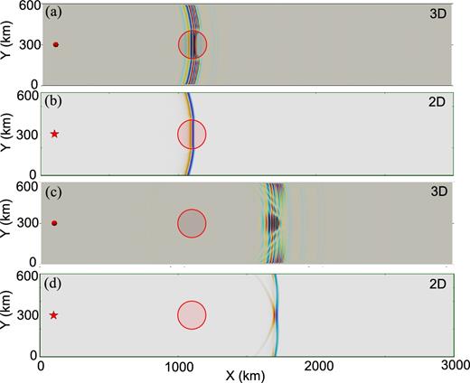
Wavefield snapshots extracted from the 3-D and 2-D simulations through a circular low-velocity anomaly or ‘basin’ for the simulation geometries shown in Fig. 12. (a) and (b) Distortion of wave front inside the basin for the 3-D and 2-D cases, respectively. (c) and (d) Amplification (focusing) and the generation of a secondary wave front for the 3-D and 2-D cases. The 3-D wavefield is more protracted in time due to surface wave dispersion.
To perform a quantitative comparison between the 2-D and 3-D wavefields, we measure spectral amplitudes at 10 s period for the 2-D and 3-D synthetics and compare them directly in Fig. 14. The amplitude measurements are normalized to the value observed at 500 km. The red vertical rectangle in the figure indicates the location of the sedimentary basin and the low-velocity anomaly. The dominant features of the 2-D and 3-D results are consistent with each other: they both predict similar amplitude anomalies downstream from the basin, which we conclude is a 2-D focusing phenomenon. Both simulations depict amplification inside the basin, although the differences inside the basin are somewhat larger than outside the basin. We also observe an oscillation pattern of the 3-D amplitude curve relative to the 2-D results, wherever there is an abrupt change in the surface wave eigenfunctions. Consistent with results presented in Fig. 11, we believe these oscillations are caused by the interference of multimode surface waves in the 3-D simulation, which are not simulated in the 2-D computation. The results in Fig. 14 also imply that, for the 10 s Rayleigh wave (vertical component), amplification caused by focusing is much larger than the site response inside basin. This is consistent with Bowden & Tsai (2017), who investigated the site amplification effect inside sedimentary basins both analytically and numerically. Their results show that site amplification is small for the 10 s Rayleigh wave (vertical component).
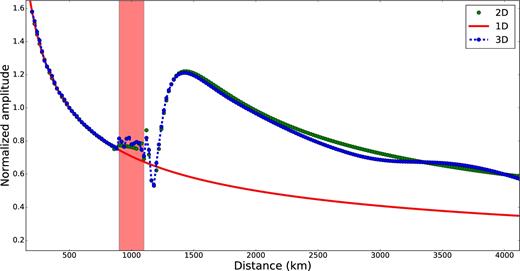
Normalized amplitudes obtained at 10 s period from the 2-D and 3-D simulations (green dots: 2-D amplitudes, blue dots with dashed line: 3-D amplitudes and red line: 1-D (horizontally homogeneous) amplitudes). The simulation geometries for the 2-D and 3-D cases are shown in Fig. 12 and wavefield snapshots in Fig. 13. The coloured box indicates the distance range of the low-velocity ‘basin’.
In summary, we first hypothesize that 2-D focusing dominantly governs the amplitude of short period surface waves propagating in a 3-D Earth, and then we use a variety of 2-D and 3-D simulation results to test the hypothesis. This conclusion is significant because it implies that the dominant residual effect of sedimentary basins on through-passing surface wave is not a complicated 3-D phenomenon as some researchers may suggest. The conclusion also means that phase velocity maps can be used to make amplitude predictions. This is not only computationally much faster, but phase velocity maps are a more direct observable than 3-D models, which are inferred from phase velocity maps and perhaps other data. Also, accurate 3-D simulations of short-period seismic waves through water layers (e.g. Japan Sea) are challenging (e.g. Komatitsch et al.2000), but can be circumvented with 2-D membrane wave modeling.
6 FURTHER DISCUSSION OF ELASTIC FOCUSING
Here, we discuss other issues related to the elastic focusing of surface waves, which include: does the focusing effect diminish with distance? How does the scale and geometry (e.g. aspect ratio) of sedimentary basins affect focusing? Compared with anelastic attenuation, does focusing have a larger impact on amplitude?
6.1 Wave front healing
The simulation results presented in Fig. 14 show decay of the surface wave amplification downstream from the anomaly. This decay results from wave front healing (e.g. Nolet & Dahlen 2000), which is a diffraction phenomenon consistent with Huygens’ principle that causes wave front distortion and amplification to decay with distance downstream from the basin. In contrast with body waves (Marquering et al.1999), where the traveltime perturbation asymptotically approaches zero at large propagation distances, surface waves undergo only incomplete healing of both traveltime and amplitude perturbations irrespective of the epicentral distance. This phenomenon is reflected in 2-D surface wave sensitivity kernels, which do not go to zero at the centre of the kernel (Fig. 15) unlike the 3-D body wave traveltime kernel.

Cross-sections of 2-D surface wave sensitivity kernels, shown to illuminate wave front healing. (a) Cross-section of the traveltime kernel, (b) cross-section of the amplitude kernel. (Sensitivity kernels are not used in any of the quantitative analysis presented here).
6.2 Effects of basin size/geometry on surface wave focusing
6.2.1 Effect of basin size
Surface wave focusing depends on the size of basin (low-velocity anomaly). To illustrate this, we present several 2-D membrane wave simulations with circular anomalies of different diameters. In the numerical scheme, the distance from the source to the centre of the circular velocity anomaly is 3000 km. The fractional wave speed perturbation of the anomaly is given by eq. (4) with ε = − 10 per cent. We vary the radius of the anomaly, which is R in eq. (4), incrementally from 100 to 400 km in the different simulations.
The amplitude curves for different simulations are presented in Fig. 16(a) from which we draw two conclusions.
The maximum amplitude downstream from the basin increases as the size of the basin grows. When the size of the basin increases, the primary wavefield out distances the secondary wavefield by a larger amount than for a smaller basin, which increases the curvature of the diffracted part of the wavefield and increases the amplitude. This is summarized in Fig. 16(b), which shows both the increase in the maximum amplitude with the size of the basin and the increase in the maximum ratio between the observed amplitude and the amplitude of the wavefield without the basin, which we call the maximum amplitude ratio. The maximum amplitude increases sublinearly with the size of the basin, whereas the maximum amplitude ratio changes more linearly with the size of the basin.
- The location of the maximum amplitude also changes with basin radius. If the incoming wave front were perfectly planar, the location of the maximum amplitude would be the focal point. However, the incoming wave front is only approximately planar. To estimate the focal length of the velocity anomaly for the non-planar incoming wave front, we use the thin lens equation. If we define the image distance (di) as the distance from the centre of the velocity anomaly to the location of the maximum amplitude, we can approximately determine the focal length using the thin lens formula:where do = 3000 km is the object distance from the source to the centre of the basin, and f is the focal length to be computed. Fig. 16(c) shows that the focal length defined in this way increases approximately linearly with the radius of the basin (blue dots: computed focal length from eq. (6) and black line: linear regression curve). This analysis is only approximately valid, because a circular low-velocity anomaly is not an ideal thin lens and it is not expected to have a single focus. Also, the lens equation is ray theoretical, which may be inappropriate in the presence of strong diffraction as exists in these simulations.(6)\begin{equation} \frac{1}{{{d_i}}} + \frac{1}{{{d_o}}} = \frac{1}{f} \end{equation}
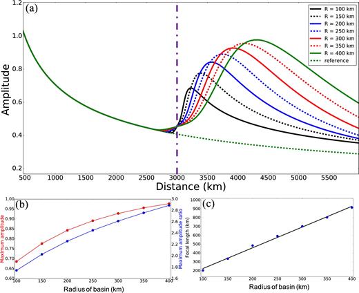
(a) Amplitude measurements from 2-D simulations through circular low-velocity anomalies or ‘basins’ with radii ranging from 100 to 400 km. (b) The maximum amplitude and maximum amplitude ratio plotted as a function of the radius of the basin. Amplitude ratio is the amplitude in the simulation with the basin divided by the amplitude in the laterally homogeneous model. (c) The focal length is computed using eq. (6). The blue dots are the computed values and the black curve is the linear regression curve.
6.2.2 Effect of basin shape
We now discuss the effect of the shape of the basin on surface wave amplitudes by presenting two examples. Fig. 17 shows surface wave amplitudes measured in a 2-D membrane wave simulation through a rectangular low-velocity anomaly centred 1000 km from the source. The aspect ratio of the velocity anomaly is extremely small; that is, the long direction of the anomaly (perpendicular to the direction of propagation) is much greater than the short direction (along the direction of propagation). In this case, there is almost no amplification downstream from the basin, as shown in Fig. 17(b), although there is amplification inside the basin, which is caused by the stacking up of the waves as they slow down. Amplification caused by focusing is due to the bending of the wave front, but when a plane wave hits an anomaly that is very long in the direction transverse to the propagation direction, the wave front will not bend, which is why there is little focusing.
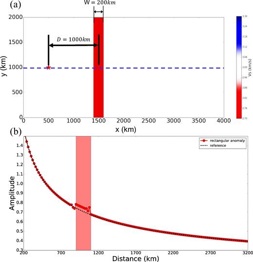
The first 2-D membrane wave simulation to contrast with Fig. 16 to illustrate the importance of the shape of the velocity anomaly or ‘basin’. (a) Source location (red star) and position of the basin (red rectangle with the long axis in the vertical direction, normal to the long axis in the wave propagation direction). The receivers are aligned along the blue dashed line. (b) The amplitude measurements obtained through the basin in (a).
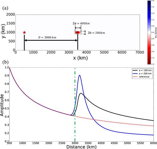
The second 2-D membrane wave simulation to contrast with Fig. 16 to illustrate the importance of the aspect ratio of the velocity anomaly or ‘basin’. (a) Source location (red star) and position of the basin (red ellipse with an aspect ratio of two). (b) The blue curve represents amplitude measurements obtained through the low-velocity basin in (a), while the black one is the amplitude predictions generated from a basin with a semimajor axis of 100 km (a = b = 100 km, which is a circular basin). The red dashed line is the reference amplitude curve for a horizontally homogeneous media, while the green dashed line indicates the centre of basin.
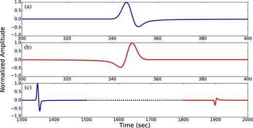
Synthetic seismograms extracted from the 2-D membrane wave simulation with an elliptical low-velocity anomaly or ‘basin’, the amplitude for each waveform has been normalized. (a) Seismogram extracted at a source–receiver distance of 1000 km. (b) Inverse Hilbert transformed version of (a). (c) Seismogram extracted at a source–receiver distance of 4000 km in which the primary and secondary wave packets are well separated.
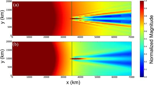
Normalized amplitude maps extracted from the 2-D membrane wave simulation with an elliptical low-velocity anomaly or ‘basin’. (a) Amplitude map measured based on FTAN. (b) Amplitude map measured based on eq. (7), which captures all of the energy in the wavefield. The vertical green line indicates the centre of basin.
In summary, a rule of thumb is that amplification strengthens and the focal length increases when the size of the low-velocity anomaly increases, approximately linearly for a low-velocity basin with an aspect ratio near 1. However, this relation breaks down for basins with extreme aspect ratios.
6.3 Anelastic attenuation versus elastic focusing
The simulations we have presented so far emphasize the effect of near-surface elastic heterogeneity on surface wave amplitudes. Now, for comparison, we address the effect of anelastic attenuation by presenting more 3-D simulations using the code SW4. (None of the simulations in this subsection are in 2-D.)
The quality factor Q is lower in sedimentary than non-sedimentary rocks, thus strong anelastic attenuation will decrease amplitudes of surface waves that pass through sedimentary basins, somewhat offsetting amplitude gains caused by elastic structures. Here, we show that the amplification effect due to focusing is expected to be much larger than the attenuation effect due to the anelasticity, at least for basins with an aspect ratio near 1.
The model parameters inside the basin for the three input models are summarized in Table 2 and are described as follows. Model 1 has both elastic and anelastic heterogeneity: a low Vs/Vp, low Q basin. Model 2 has only elastic heterogeneity: a low Vs/Vp but normal Q basin. Model 3 has only anelastic heterogeneity: a normal Vs/Vp but low Q basin. Thus, Model 1 contains both a Vs/Vp and Q anomaly, Model 2 contains only a Vs/Vp anomaly and Model 3 contains only a Q anomaly. Our main interest is to compare the results of Models 2 and 3, which contain purely elastic and purely anelastic effects, respectively.
Velocity and quality factor inside the basin for different simulations in Section 8.
| Model ID | vs | vP | Qs | QP |
|---|---|---|---|---|
| 1 – both | 2 km s−1 | 3.59 km s−1 | 40 | 96.8 |
| 2 – elastic | 2 km s−1 | 3.59 km s−1 | 600 (ak135) | 873 (ak135) |
| 3 – anelastic | 3.46 km s−1 (ak135) | 5.8 km s−1 (ak135) | 40 | 96.8 |
| Model ID | vs | vP | Qs | QP |
|---|---|---|---|---|
| 1 – both | 2 km s−1 | 3.59 km s−1 | 40 | 96.8 |
| 2 – elastic | 2 km s−1 | 3.59 km s−1 | 600 (ak135) | 873 (ak135) |
| 3 – anelastic | 3.46 km s−1 (ak135) | 5.8 km s−1 (ak135) | 40 | 96.8 |
We use the amplitude ratio in Fig. 21(a) to illustrate the results, which is the ratio of observed amplitude in the simulation (Aobs) to the reference amplitude observed with the horizontally homogeneous model ak135 (Aref). Strong anelastic attenuation (Model 3) alone only decreases amplitudes to a small extent (red dots). The elastic structural anomaly (Model 2) has a much larger effect on amplitudes downstream from the basin (green dots). A basin that has both low-velocity and low-quality factors (Model 1) still results in a significant increase in the amplitudes downstream from the basin (blue dots).
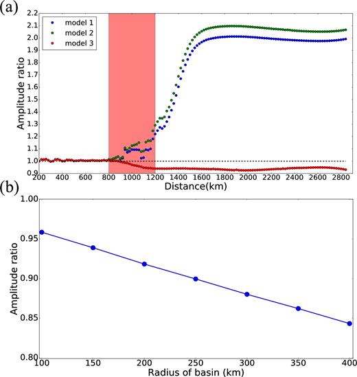
(a) Amplitude ratio from three 3-D simulations with different input models with varying amounts of elastic and anelastic heterogeneities. Model 1: both elastic and anelastic heterogeneities, Model 2: only elastic heterogeneity, Model 3: only anelastic heterogeneity. A full description of the models is summarized in Table 2. (b) Anelastic amplitude ratio is plotted as a function of the radius of the basin, where the anomaly is purely anelastic (i.e. no elastic heterogeneity).
Fig. 21(b) shows that the magnitude of the downstream amplitude anomalies in simulations with a purely anelastic heterogeneity varies approximately linearly with the size of the basin, as does the maximum elastic amplitude ratio (Fig. 16b). However, the anelastic effect is much smaller. As shown in Fig. 21(a), for a basin with a radius of 200 km, the magnitude of anelastic amplitude decay would be ∼7 per cent, but the maximum elastic amplification would be ∼200 per cent. Thus, the expectation is that elastic amplification effects will have larger impact than anelastic attenuation effects for basins with an aspect ratio near 1.
There are three primary exceptions to the dominance of elastic amplification over anelastic attenuation. (1) Anelastic attenuation begins to set on as soon as the wavefield enters the basin and persists approximately constant downstream after the wavefield exists the basin. Elastic amplification does not set on immediately, but maximizes past the focal point which will occur several hundred kilometres downstream from the basin and then decays slowly (Fig. 16a). This caveat is more important for large basins whose focal point lies at a greater distance from the basin. For a basin with a 400 km radius, anelastic attenuation will be stronger than elastic amplification within about 250 km from the basin edge in our simulations, but will be weaker outside this distance. (2) Elastic amplification reduces downstream from the focal point, whereas anelastic attenuation remains constant with distance. Thus, for waves that propagate far enough from a basin the elastic amplification may decay to become commensurate with anelastic attenuation. This will be more likely for small basins where the amplification decays more rapidly with distance. However, elastic focusing does not asymptotically approach zero (as discussed earlier). Even for a basin that is only 100 km in radius, the elastic focusing is expected to be much stronger than anelastic attenuation at continental scales (distances less than 10,000 km). (3) For basins with extreme aspect ratios, such as shown in Fig. 17, elastic focusing may be minimal and anelastic attenuation may have a larger impact on amplitudes simply because there is negligible focusing. (4) For an elliptical basin, the wavefield propagating through the long axis may separate into two wave packets. Although focusing of energy still occurs (as shown in Fig. 20b), the measured amplitude based on conventional methods may not accurately reflect the amplification of wavefield energy (as shown in Fig. 20a). In this case, it is hard to determine whether focusing has a larger impact compared with anelastic attenuation or not.
In conclusion, we expect elastic amplification downstream from on-continent sedimentary basins to dominate anelastic attenuation except very near the basin edge and for basins with extreme aspect ratios.
7 CONCLUSIONS
This paper explores the nature of elastic propagation effects on short-period surface waves, particularly their amplitudes downstream from sedimentary basins. Our results show that a significant fraction of amplitude variability observed in regionally propagating surface waves (e.g. Bonner et al.2008) is caused by elastic focusing/defocusing due to lateral wave propagation effects through shallow structures. The focus of this paper is to understand elastic focusing effects on Rayleigh waves at 10 s period, which is typically well excited by small earthquakes and nuclear explosions and is also well represented in ambient noise cross-correlations that are commonly used in tomographic studies. The existence and nature of sedimentary basins strongly affect regionally propagating Rayleigh waves at this period.
The primary findings of this paper are summarized as follows:
With the example of a 3-D full-waveform simulation across East Asia, we illustrate that elastic velocity heterogeneity of sedimentary basins has a large impact on short-period surface wave amplitudes. Ignoring these effects may introduce significant bias in studies that require the correct interpretation of amplitude information, including attenuation tomography and source parameter estimation. We also present an example of Ms estimates to highlight the amplitude variability caused by velocity heterogeneity.
We conclude that the amplitude effect of short-period surface wave propagation in a 3-D Earth is predominantly governed by horizontal 2-D focusing/defocusing, rather than complicated 3-D wave propagation phenomena. Several pieces of numerical evidence are provided to establish this conclusion, which is particularly useful due to the fact that 2-D phase speed maps can be used as proxy for 3-D structural models to predict surface wave amplitude anomalies. There are several reasons we believe 2-D simulations through phase velocity maps may be preferable to 3-D simulations. First, 2-D membrane wave simulations are much faster. Second, the existence of water layers can complicate simulations through a 3-D model that does not happen in 2-D simulations. Third, phase speed maps are closer to data than 3-D models and are, therefore, more accurate representations of heterogeneity. Thus, phase speed maps present several advantages in computing amplitude predictions, including that they may be more accurate than those computed through a 3-D model.
Several important questions related to the nature of the 2-D focusing effect are discussed in detail. Most importantly, we compare the effects of anelastic attenuation to elastic focusing and show that on a regional scale elastic focusing through sedimentary basins is more likely to cause significant surface wave amplitude anomalies than anelastic attenuation produced by sedimentary basins except very near the basin edge or for basins with extreme aspect ratios. This explains why negative values of Qeff are commonly observed in observational studies (e.g. Levshin et al.2010).
In the future, it is important to test the principal conclusions of this paper with real data. This will include tests to observe strong lineations or amplification stripes downstream from sedimentary basins, and perhaps also the de-amplification and propagation deflection stripes that bracket the amplification. In addition, it is also important to test whether the observed features are predicted well with high-quality velocity models. To achieve this, there are three major requirements that need to be satisfied. (1) A dense array with high-quality seismometers is needed to record accurate spatially resolved amplitude information. The array should be located near to a large sedimentary basin. (2) Seismic events upstream from the basin are also needed with magnitudes large enough to be recorded by the array. Ideally, they should also be small enough and far enough to be considered as point sources. (3) A high-resolution 3-D model (or 2-D phase velocity maps) also should be available for the study region.
Acknowledgements
The authors thank an anonymous reviewer and Art Frankel for constructive criticisms that helped to improve the paper substantially, and Weisen Shen and Michael Pasyanos for insightful discussions that helped to motivate this work. We are also grateful to Michael Pasyanos for providing the Ms measurements for the 2006 DPRK Nuclear Test. We thank the authors of the following software packages for making codes freely available: SES3D, SPECFEM2D, SW4, FMST and Computer Programs in Seismology. In particular, we are grateful to Andreas Fichtner for answering technical questions about the code SES3D. Without these codes this study could not have been completed. Figures in this paper are produced using Matplotlib Basemap Toolkit and the data processing strongly relies on ObsPy (Beyreuther et al. 2010). Aspects of this research were supported by NSF grant EAR-1645269 and Air Force Research Laboratory contract no. FA9453-13-C-0278 at the University of Colorado at Boulder. This work utilized the Janus supercomputer, which is supported by the National Science Foundation (award number CNS-0821794), the University of Colorado at Boulder, the University of Colorado Denver and the National Center for Atmospheric Research. The Janus supercomputer is operated by the University of Colorado at Boulder.
REFERENCES
SUPPORTING INFORMATION
Supplementary data are available at GJI online.
EA_wavefield.avi
Please note: Oxford University Press is not responsible for the content or functionality of any supporting materials supplied by the authors. Any queries (other than missing material) should be directed to the corresponding author for the paper.
