


Abstract
This paper develops and applies a Bernstein-polynomial parametrization to efficiently represent general, gradient-based profiles in nonlinear geophysical inversion, with application to ambient-noise Rayleigh-wave dispersion data. Bernstein polynomials provide a stable parametrization in that small perturbations to the model parameters (basis-function coefficients) result in only small perturbations to the geophysical parameter profile. A fully nonlinear Bayesian inversion methodology is applied to estimate shear wave velocity (VS) profiles and uncertainties from surface wave dispersion data extracted from ambient seismic noise. The Bayesian information criterion is used to determine the appropriate polynomial order consistent with the resolving power of the data. Data error correlations are accounted for in the inversion using a parametric autoregressive model. The inversion solution is defined in terms of marginal posterior probability profiles for VS as a function of depth, estimated using Metropolis–Hastings sampling with parallel tempering. This methodology is applied to synthetic dispersion data as well as data processed from passive array recordings collected on the Fraser River Delta in British Columbia, Canada. Results from this work are in good agreement with previous studies, as well as with co-located invasive measurements. The approach considered here is better suited than ‘layered’ modelling approaches in applications where smooth gradients in geophysical parameters are expected, such as soil/sediment profiles. Further, the Bernstein polynomial representation is more general than smooth models based on a fixed choice of gradient type (e.g. power-law gradient) because the form of the gradient is determined objectively by the data, rather than by a subjective parametrization choice.
1 INTRODUCTION
The level of shaking experienced during an earthquake is strongly dependent upon the local, near-surface geophysical properties. In particular, as seismic waves propagate through material of decreasing impedance, the resistance to motion decreases and wave amplitude increases (Anderson et al. 1986, 1996). Amplification can also occur at particular frequencies due to resonance within near-surface low-velocity layers or 3-D basin structures (Bard & Bouchon 1980; Graves et al. 1998). Knowledge of the local, near-surface geophysical properties is critical for understanding seismic amplification and resonance hazards (e.g. Molnar et al. 2013; Adams et al. 2015). The shear wave velocity (VS) profile over the upper tens of metres is representative of the soil/sediment rigidity at a site, and can be used to predict the expected ground response to earthquake shaking. Thus, estimating VS is important for seismic site classification and studies of public safety related to earthquake hazards. The VS profile at a site can be determined by invasive methods such as boreholes or seismic cone penetration tests (SCPT), or can be estimated from non-invasive, active or passive seismic observations made at the surface. Passive methods involving small, portable, 2-D seismic arrays are increasingly popular because they often have lower demands in cost and logistics compared to other methods (e.g. Aki 1957; Lacoss et al. 1969; Wathelet et al. 2008; Molnar et al. 2010). This technique involves processing the array recordings of ambient seismic noise to estimate the phase velocity of fundamental-mode Rayleigh waves as a function of frequency (the dispersion curve), which can be inverted to estimate the VS profile and, with very low resolution, the compressional-wave velocity (VP) and density (ρ) profiles.
Understanding and quantifying the uncertainties in estimated VS profiles, and their effects on seismic site classification uncertainties, is of significant interest to developers, planners, and public officials internationally and has been identified as a critical issue for passive seismic array methods (Cornou et al. 2006). Bayesian inference provides a rigorous approach to uncertainty quantification for nonlinear inverse problems (like dispersion inversion). Bayesian inversion is a probabilistic approach in which the parameters that describe the model (e.g. the VS profile) are constrained by the observed data and prior information. The solution is described by properties of the posterior probability density (PPD) of the model parameters, which is generally estimated numerically using Markov-chain Monte Carlo (MCMC) methods (Mosegaard & Tarantola 1995; Brooks et al. 2011). Within a Bayesian framework, the most probable VS profile as well as quantitative measures of the profile uncertainty can be determined from the PPD. Nonlinear Bayesian inversion provides a rigorous approach to quantifying uncertainties which avoids linearization errors and subjective regularizations that can preclude meaningful uncertainty analysis in linearized approaches. Bayesian inversion has been applied previously to dispersion data processed from passive array recordings (Molnar et al. 2010; Dettmer et al. 2012; Molnar et al. 2013).
In any inversion, an appropriate parametrization is required to describe the model that represents the physical system of interest (in this case, the VS profile). Molnar et al. (2010) considered Bayesian inversion of array dispersion data using parametrizations described by linear and power-law functional forms to represent VS gradient structures in near-surface soils/sediments. Results in good agreement with borehole and SCPT measurements were obtained, but in this approach the profile form (power-law or linear gradient) is imposed on the solution rather than determined from the data. Furthermore, while these gradient forms are often reasonably applicable, they have limited flexibility to capture general earth structure. In many geophysical inversion approaches, earth-structure profiles are parametrized as a stack of homogeneous layers. Dettmer et al. (2012) considered Bayesian inversion of the same data using a trans-dimensional (trans-D) model parametrization based on homogeneous layers, where the dimension of the model (number of layers) is treated as unknown and sampled probabilistically within the inversion (Green 1995). This approach is designed to treat unknown parametrizations objectively and includes parametrization uncertainty within the profile uncertainty estimates. However, this may not be an appropriate parametrization in cases where smooth gradients are expected, and can introduce non-physical discontinuities in the inversion result. Furthermore, dispersion data are typically not sensitive to fine-scale discontinuous structure due to the diffusive nature of surface waves.
This paper considers a general and efficient approach to parameterizing smooth gradient-based profiles (over an impedance contrast) in terms of a Bernstein polynomial representation (Quijano et al. 2016). A Bernstein polynomial is defined as a weighted sum of Bernstein basis functions, which are themselves polynomials with several desirable features for representing general smooth functions (Farouki & Rajan 1989; Farouki 2012). The Bernstein basis functions are pre-defined for a given polynomial order, and the inversion estimates the coefficients which weight the individual basis functions. In this way, general gradient-based VS structure can often be represented using fewer parameters than a classical layered model parametrization. The distinctive advantageous property of the Bernstein polynomial over other polynomial forms (e.g. splines) is its stability. Specifically, small perturbations to the model parameters (basis-function coefficients) result in only small, localized perturbations to the VS profile. In fact, the Bernstein polynomial has optimal stability for a given polynomial order (Farouki & Rajan 1989; Farouki 2012).
Bernstein polynomials were originally formulated for applications in theoretical mathematics with later applications in computer-aided design, differential-equation solutions, and control theory (Gordon & Riesenfeld 1974; Bhattia & Bracken 2007; Farouki 2012; Basirat & Shahdadi 2013). Quijano et al. (2016) parametrized a seabed geoacoustic model using a Bernstein polynomial in Bayesian inversion of ocean-acoustic bottom-loss data. This paper introduces the Bernstein polynomial parametrization to geophysical inversion by estimating VS profiles from fundamental-mode Rayleigh wave dispersion data within a Bayesian framework. This methodology is applied to synthetic dispersion data as well as passive-array data recorded on the Fraser River Delta in British Columbia (BC), Canada.
2 BAYESIAN INVERSION METHODOLOGY
This section provides an overview of the Bayesian inversion theory and implementation used in this study, as well as a description of the treatment of prior knowledge and data errors. More complete reviews of Bayesian inversion can be found in Tarantola (2005) and Brooks et al. (2011).
In this work, the data are treated in terms of slowness (the reciprocal of phase velocity) as passive array methods applied here typically estimate the wavenumber of propagating surface waves, and errors in slowness scale linearly with errors in the estimated wavenumber. For slowness errors of the same variance within a given data subset (frequency band), this has the effect of increasing phase-velocity errors at low frequencies (relative to higher frequencies) since dispersion data generally have higher phase velocities at low frequencies. This is believed to be a more physically reasonable representation of the frequency dependence of the data errors than previous work which treated phase velocities as data (Molnar et al. 2010; Dettmer et al. 2012).
3 MODEL PARAMETRIZATION
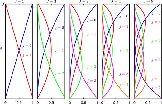
Basis functions for Bernstein polynomials of orders J = 1 to 5.
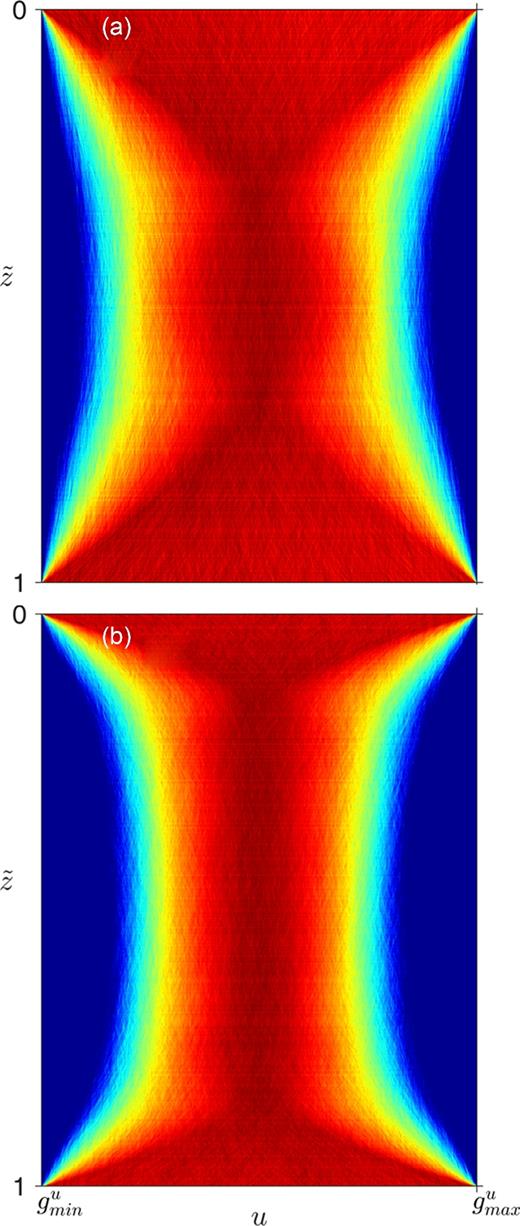
Prior density profiles for parameter u using Bernstein polynomials of order (a) Ju = 2 and (b) Ju = 5. Warm colours (red) represent high probability and cool colours (blue) represent low probability. Probabilities are normalized independently at every depth for display purposes.
4 SIMULATION STUDY
Performing inversions on simulated data which correspond to a known true model (with a known error process on the data) is a useful test for examining the effects of specific inversion methodologies (e.g. comparing different model parametrizations). This section illustrates the Bernstein-polynomial parametrization using simulated Rayleigh-wave dispersion data computed for an earth structure model with VS increasing with depth according to a power-law, overlaying a linear gradient, overlaying a half-space (with uniform VP/VS). A high-quality data set of 40 logarithmically spaced slowness values were computed between 2 and 12 Hz. Correlated errors were simulated using Gaussian-distributed errors with standard deviation 10−4 s m−1 (in slowness) and AR parameter 0.6 over a single data subset. Hence, only a single data subset is considered in the inversion (i.e. ND = 1 in eq. 7). Bayesian inversions were carried out using the methodology described above as well as using the trans-D layered approach of Dettmer et al. (2012), and the power-law model approach of Molnar et al. (2010). In all cases the same error model (AR parameter and unknown variance) was applied so the comparisons isolate the effects of the choice of model parametrization on the inversion results. The model parameter prior bounds for each inversion are shown in Table 1. Fig. 3 shows the results of the BIC analysis performed for the Bernstein-polynomial approach. The BIC is a minimum for |$J^{V_{S}} = 5$| and |$J^{V_{P}/V_{S}} = 1$|, so the final inversion results are shown for this parametrization.
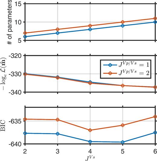
BIC analysis for synthetic dispersion data. The likelihood of the MAP model |${\cal L}({\bf \hat{m}})$| and number of model parameters are also shown as functions of Bernstein-polynomial order.
Prior bounds for model parameters in Bernstein-polynomial, trans-D and power-law inversions of synthetic dispersion data.
| Bernstein parameter | Min | Max |
| |$g^{V_{S}}$| (m s−1) | 50 | 1000 |
| |$g^{V_{P}/V_{S}}$| | 1.4 | 3 |
| z0 (m) | 20 | 150 |
| Half-space VS (m s−1) | 500 | 1000 |
| Half-space VP/VS | 1.4 | 3 |
| a | 0 | 0.9 |
| Trans-D parameter | Min | Max |
| Layer VS (m s−1) | 50 | 1000 |
| Layer VP/VS | 1.4 | 3 |
| Layer depth (m) | 0 | 150 |
| Number of layers | 2 | 20 |
| a | 0 | 0.9 |
| Power-law parameter | Min | Max |
| VS at 1 m depth (m s−1) | 50 | 500 |
| VS at z0 (m s−1) | 200 | 1000 |
| VP/VS at 1 m depth | 1.4 | 3 |
| VP/VS at z0 | 1.4 | 3 |
| z0 (m) | 20 | 150 |
| Half-space VS (m s−1) | 500 | 1000 |
| Half-space VP/VS | 1.4 | 3 |
| a | 0 | 0.9 |
Fig. 4 shows the fit to the data from the inversions (plotted as phase velocities, although slownesses were inverted). All inversions provide a good fit to the dispersion data, with similar variance in dispersion data produced for models in the Markov chains. The main results for the inversion are considered in terms of marginal probability profiles for VS using the Bernstein-polynomial, trans-D, and power-law model parametrizations (Fig. 5). The solid lines represent the profile of VS used to generate the synthetic dispersion data (i.e. the true model). The inversion results for VS using the Bernstein-polynomial model are in good agreement with the true model, and the form of the profile (smooth, continuous function of depth above the half-space) is well represented. The trans-D inversion, shown in Fig. 5(c), produces VS values which are generally close to the true values; however, the recovered profile indicates discrete, uniform layering over the upper 70 m which differs significantly from the true smooth gradients. Such layering is not required to fit the data, but is a consequence of the choice of model parametrization. The trans-D approach has the added benefit of including the model complexity (number of layers) as an unknown in the inversion. As a result, the uncertainty of the parametrization is included within the estimated PPD. This property, combined with the fact that the trans-D inversion requires more parameters (thickness, VS, and VP/VS values in up to 20 layers) than the Bernstein polynomial, are likely why the uncertainties appear larger in the trans-D inversion results. The power-law inversion, shown in Fig. 5(e), produces VS values which are in excellent agreement with the true values down to approximately 40 m depth, the onset of the linear gradient, due to the correct prior assumption on the form of the VS profile. The Bernstein-polynomial inversion results (Fig. 5a) also produces VS values which agree with the true values since this structure is constrained by the data information, not a fixed prior assumption. However, the Bernstein inversion results have increased uncertainties in the near surface (less than 10 m depth) compared to the power-law inversion. This result is expected and is a physical limitation of the frequency band of the dispersion data. The decreasing near-surface uncertainties in the power-law inversion come from the prior (not the data), since this parametrization forces VS to zero at zero depth (hence, low uncertainties near the surface). This may be undesirable in applications without strong confidence in the prior. Beyond about 40 m depth, the power-law inversion is not able to represent structure which deviates from the gradient form of the power law. However, the dispersion data clearly contain information on the VS structure beyond 40 m depth as the Bernstein-polynomial inversion results accurately capture the change in gradient form. Furthermore, the unrealistically small uncertainties in VS estimated by the power-law inversion compared to the other inversions suggests this inversion is underparametrized (only two parameters are required to model a power law profile).
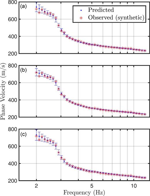
Fit to synthetic dispersion data using (a) Bernstein, (b) trans-D and (c) power-law model parametrizations. The red stars are the synthetic data (with added errors), and the blue dots are the mean predicted data (with two standard deviation error bars) from the MCMC samples.
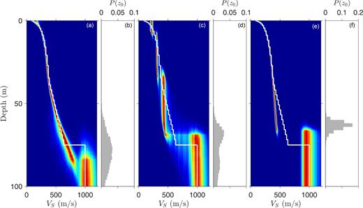
Marginal probability profiles for VS, and marginal probability densities for z0, from inversions of synthetic data using the (a,b) Bernstein, (c,d) trans-D and (e,f) power-law model parametrizations.
Fig. 6 shows the most probable VS profiles from the Bernstein, trans-D, and power-law inversions in comparison with the true model. For the Bernstein and power-law inversions, the MAP model is shown. In the case of the trans-D inversion, the model which minimizes the BIC (as described in the previous section) is shown since the MAP model would be a high-dimension, overparametrized solution. Furthermore, the MAP model is not well defined in trans-D inversion since the PPD for different dimensions has different units, and cannot be directly compared. Fig. 7 shows the marginal probability profiles for VP/VS using the Bernstein-polynomial, trans-D, and power-law model parametrizations. As expected, dispersion data are not as sensitive to VP/VS as VS. Consequently, VP/VS structure is not well constrained in the inversions and is not considered further here.
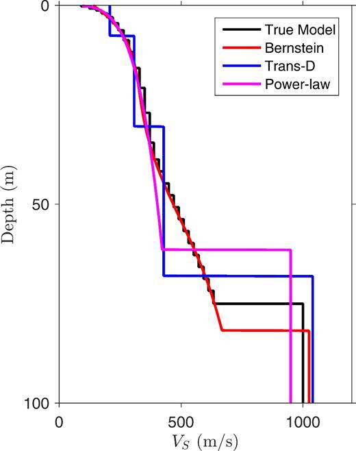
Most probable VS profiles from inversions of synthetic data using the Bernstein, trans-D, and power-law model parametrizations.

Marginal probability profiles for VP/VS from inversions of synthetic data using the (a) Bernstein, (b) trans-D and (c) power-law model parametrizations.
It can be challenging to interpret the estimated depth of the half-space (basement) z0 from marginal probability profiles for VS. Figs 5(b), (d) and (f) show the marginal probability densities for z0 using the Bernstein polynomial, trans-D, and power-law model parametrizations, respectively. In this synthetic test, the Bernstein polynomial inversion provides the most accurate estimate of z0 (peak of the probability density), whereas the trans-D and power-law inversions estimate z0 values to shallower than the true value. Larger uncertainties in z0 are estimated using the Bernstein polynomial approach. This is likely attributed to the flexibility of the Bernstein polynomial representation compared to the other model parametrizations considered here.
This simulation study illustrates that a layered model parametrization may not be the ideal choice for studies where gradient structure in geophysical properties are of particular interest. This is evidenced by the inability of trans-D inversion to capture near-surface strong-gradient structure as well as the inclusion of large non-physical VS discontinuities in the inversion results. However, the Bernstein-polynomial parametrization can potentially miss sharp transitions at sites where unknown VS discontinuities do exist above the basement. These could be accommodated by considering a model composed of more than one Bernstein polynomial over depth, but that approach is not considered in this paper. Overall, the Bernstein-polynomial model provides a much more flexible and general representation of gradient structure (with more realistic uncertainty estimates) than other gradient-based models with fixed prior assumptions of the gradient form.
5 FRASER RIVER DELTA INVERSIONS
This section considers the inversion of Rayleigh-wave dispersion data extracted from passive array recordings from the Fraser River Delta near Vancouver, BC (Fig. 8), which were originally considered by Molnar et al. (2010). The delta is composed of up to 300 m of unconsolidated Holocene deltaic sediments from the Fraser River overlying harder Pleistocene glacial material. The combination of the proximity to the northern extent of the Cascadia subduction zone and the thick sequence of deltaic sediments results in significant amplification and liquefaction hazards in this region (Hunter et al. 1998). The data were recorded on five portable broad-band three-component seismographs which were arranged in six array configurations with station separation distances ranging from 5 to 180 m (inset of Fig. 8d). The passive array recordings were processed by Molnar et al. (2010) to produce 52 approximately logarithmically spaced dispersion data between 1.2 and 6.5 Hz. Similar to Molnar et al. (2010), the dispersion data are segmented according to assumed changes in error processes related to different array configurations. Specifically, three frequency bands are specified with boundaries at 4.2 and 5.3 Hz. A different standard deviation is sampled implicitly, and a different AR parameter is sampled explicitly, within each frequency band as described in Section 2 (i.e. ND = 3 in eq. 7).
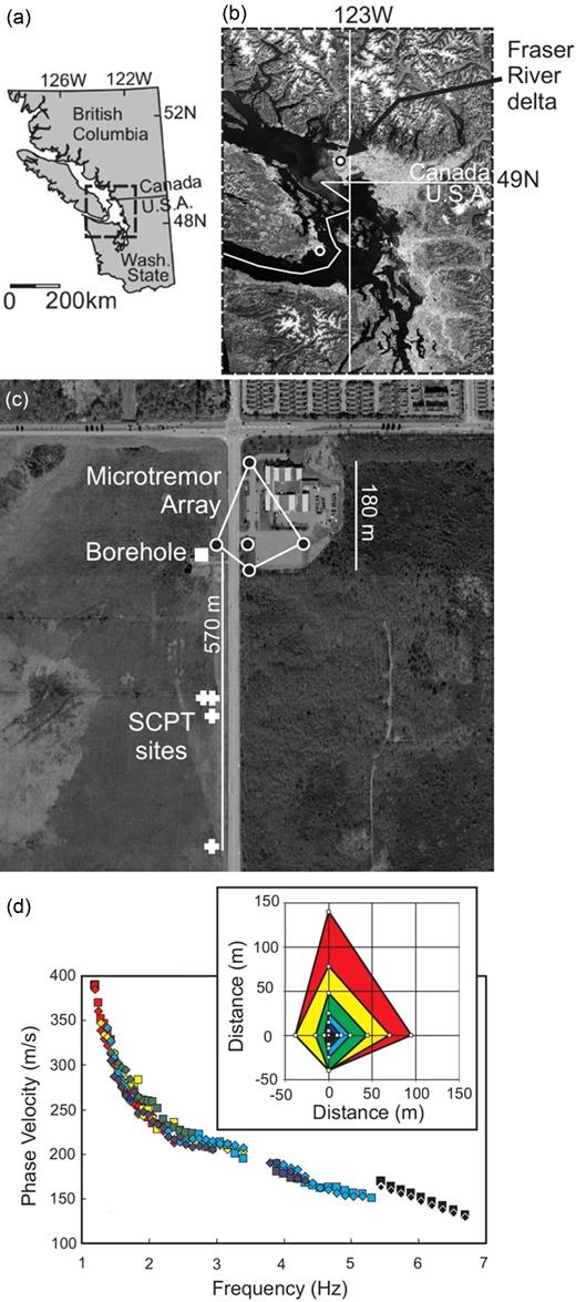
(a,b) Location of Fraser River Delta passive array site. (c) Largest array configuration and (d) processed dispersion data (data points of a particular colour were processed from the array configuration of the corresponding colour) (from Molnar et al. 2010).
In this paper, Bayesian inversion with the Bernstein polynomial parametrization is applied to these data, which have been previously considered by Molnar et al. (2010) and Dettmer et al. (2012). Model parameter prior bounds are listed in Table 2. These data are considered here as they represent a high-quality observed data set suitable for comparison with previous inversion methodologies, as well as for comparison with co-located borehole and SCPT measurements. Molnar et al. (2010) considered these data by applying Bayesian inversion with linear and power-law model parametrizations to represent gradient structures in the soils/sediments. The BIC was used to identify the power-law model as the preferred parametrization. However, the power-law parametrization has limited flexibility in representing gradient structures (as previously discussed), and this approach forces the geophysical profiles to be power laws even if the dispersion data can resolve deviations from such structure. The Bernstein-polynomial parametrization is much more general such that the form of the gradients are determined by the data, rather than by subjective parametrization choice. Dettmer et al. (2012) also considered these data by applying a trans-D Bayesian inversion such that, in every dimension, the model is represented by a discontinuous stack of uniform layers. However, discrete uniform layering structure is not expected at this site and constant lithology is believed to extend to considerable depth (Hunter & Christian 2001).
Prior bounds for model parameters in inversion of Fraser River Delta dispersion data.
| Parameter | Min | Max |
| |$g^{V_{S}}$| (m s−1) | 50 | 800 |
| |$g^{V_{P}/V_{S}}$| | 1.4 | 3 |
| z0 (m) | 20 | 200 |
| Half-space VS (m s−1) | 500 | 1500 |
| Half-space VP/VS | 1.4 | 3 |
| a | 0 | 0.9 |
| Parameter | Min | Max |
| |$g^{V_{S}}$| (m s−1) | 50 | 800 |
| |$g^{V_{P}/V_{S}}$| | 1.4 | 3 |
| z0 (m) | 20 | 200 |
| Half-space VS (m s−1) | 500 | 1500 |
| Half-space VP/VS | 1.4 | 3 |
| a | 0 | 0.9 |
Fig. 9 shows the results of the BIC analysis performed for the Bernstein polynomial parametrization. The BIC is a minimum for |$J^{V_{S}} = 3$| and |$J^{V_{P}/V_{S}} = 1$| and so the final inversion results are shown for this parametrization. Fig. 10(a) shows the marginal probability profile for VS, which represent the main results of the inversion (the marginal probability profile for VP/VS is not shown due to the lack of sensitivity of these parameters). Figs 10(c) and (e) show the marginal probability profiles for VS using the methods of Dettmer et al. (2012) and Molnar et al. (2010), respectively. The VS marginal profile from the Bernstein-polynomial inversion shows clear depth-dependent structure, with velocities increasing with depth, particularly in the near surface. The Bernstein-polynomial inversion produces a smooth, continuous gradient that is similar to a power-law (with some deviation from this fixed functional form). In particular, the Bernstein-polynomial inversion allows for VS to increase at depths greater than 120 m, where a power-law does not. The marginal probability density for z0 (Fig. 10b) indicates a transition at 140–200 m depth. Uncertainty in the VS structure generally increases with depth, as is expected from the decaying resolution of surface wave dispersion data with depth. However, uncertainties in VS increase slightly towards the surface at depths shallower than 10–15 m, indicative of a high-frequency resolution limit in the data. This effect is not as apparent as in the simulation study from the previous section due to the lower-order polynomial required in this inversion (|$J^{V_{S}} = 3$|, as opposed to |$J^{V_{S}} = 5$| in the simulation), which limits the range of possible near-surface curvature (at depths shallower than the resolution limit of the dispersion data). The dispersion inversion results are compared to invasive VS measurements from a borehole and SCPT data collected near the passive array (Fig 8c). The white dots with error bars are the mean of the available SCPT and borehole measurements ±1 standard deviation (Dallimore et al. 1995; Hunter et al. 1998; Molnar et al. 2010). The inversion results are in good agreement with the invasive VS estimates with detailed structure generally captured within the uncertainties in the inversion results. It should be noted that the inversion results represent an average solution over the lateral spatial extent of the passive array. The VS values estimated from invasive measurements represent an average of point estimates that are spatially distributed (with the greatest separation between measurements being 570 m) and not perfectly co-located with the passive array. VS values estimated from invasive measurements also have their own associated measurement errors, which are not included in the error bars in Fig. 10.

BIC analysis for Fraser River Delta dispersion data. The likelihood of the MAP model |${\cal L}({\bf \hat{m}})$| and number of model parameters are also shown as functions of Bernstein-polynomial order.
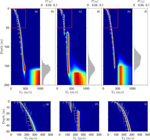
Marginal probability profiles for VS, and marginal probability densities for z0, from Fraser River Delta dispersion data using the (a,b,g) Bernstein polynomial model, (c,d,h) trans-D inversion results inversion results using the method of Dettmer et al. (2012) and (e,f,i) power-law inversion results using the method of Molnar et al. (2010). Lower panels show the near-surface VS marginal probability profiles for the range delineated in red in the main panels. The white dots are the mean (with one standard deviation error bars) of the available SCPT and borehole measurements.
The inversion results from Molnar et al. (2010) indicate near-surface VS of 70–90 m s−1 increasing to 325–425 m s−1 at the base of the modelled power-law layer, which is estimated to be 100–170 m thick overlaying a half-space (Fig. 10f). The inversion results from Dettmer et al. (2012) indicate the VS profile is composed of three layers with discontinuities at approximately 17 and 65 m depth, transitioning to a half-space at 110–200 m depth (Fig. 10d). Velocities in the near-surface layers are approximately constant with depth and are consistent with average values over the corresponding depth ranges from results from Molnar et al. (2010) as well as results from this study. There is no geological explanation for the sharp velocity discontinuities at 17 and 65 m depth, other than to model the increase in VS with depth using a layered parametrization. With all parametrization approaches, the depth and velocities in the half-space are poorly resolved with uncertainties of tens of metres and hundreds of metres per second, respectively. Depending on the geological conditions, the depth resolution limit for dispersion data processed from passive array recordings is typically taken to be on the order of the maximum station separation distance which in this case is 180 m (Park et al. 1999; Wathelet et al. 2008). It is possible (likely) that the transition to the half-space does not represent a physical discontinuity to a homogeneous layer, but instead marks the resolution limit of the dispersion data (Molnar et al. 2010).
Results from this work are generally in good agreement with previous studies. However, the results shown here allow the gradient form of the results to be determined by the data, rather than by subjective parametrization choice. In particular, the trans-D inversion results do not agree with the invasive measurements as well as the Bernstein-polynomial or power-law inversion results and is not the best type of model for this application (given prior knowledge for this site). The invasive measurements indicate that a power-law model is a good parametrization choice in this case as the power-law inversion results appear to fit the invasive measurements better than Bernstein-polynomial inversion results, due to sharper curvature in the VS profile near the surface (compare Figs 8g and i). This indicates that the prior information built into the functional form of the power-law model is approximately correct in this particular case, but may not necessarily be so in other environments. However, the Bernstein-polynomial inversion results have less near-surface curvature because the data are not able to resolve the sharper near-surface gradient. This is most likely due to the lack of high-frequency dispersion data (>6.5 Hz), which constrain shallow VS structure. The Bernstein polynomial inversion more clearly indicates the information content of the data with less influence from prior information on the gradient form, which may or may not be desired, depending on how trustworthy this prior information is believed to be.
Fig. 11 shows a good fit to the dispersion data from the Bernstein-polynomial inversion results (in fact, all inversions fit the data in a similar manner), with reasonable variance for the data predictions (plotted as phase velocities, although slownesses were inverted). To validate the assumptions for the error process, statistical tests are applied to the standardized residuals of the MAP model for the Bernstein-polynomial inversion. Fig. 12 shows the histogram and autocorrelation function of the standardized residuals of the MAP model. If the error process is Gaussian, then the histogram of the standardized residuals will approximate the standard normal Gaussian (the solid line in Fig. 12a). The Kolmogorov–Smirnov (KS) test was applied to quantitatively assess the validity of this assumption and provided a p-value of 0.26 for the null hypothesis of Gaussian-distributed errors (Freund 1967; Dosso et al. 2006). The width of the central peak of the autocorrelation of the standardized residuals (Fig. 12b) gives an indication of the correlation in data errors. Ideally, the AR model will account for correlation and the resulting standardized residuals will be uncorrelated (with a narrower central peak of the autocorrelation function). The runs test was applied to quantitatively assess the validity of this assumption and provided a p-value of 0.12 for the null hypothesis of uncorrelated errors (Freund 1967; Dosso et al. 2006). In this case, neither null hypothesis is rejected (using the typical threshold of p < 0.05 for rejection) and the data error assumptions in the inversion appear justified.
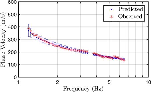
Data fit to Fraser River Delta dispersion data from Bernstein polynomial inversion. The red stars are the observed dispersion data, and the blue dots are the mean predicted data (with two standard deviation error bars) from the MCMC samples.
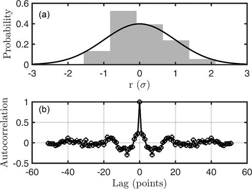
(a) Histogram and (b) autocorrelation of standardized residuals from the MAP model. The solid line in (a) is the standard normal distribution.
6 DISCUSSION AND CONCLUSIONS
This paper considered Bayesian inversion of surface wave dispersion data using a general and efficient approach to parameterizing smooth gradient-based profiles in terms of a Bernstein-polynomial representation. The Bernstein-polynomial parametrization may be better suited than parametrizations based on discrete layers for nonlinear inversions when general smooth gradients in geophysical parameters are expected, such as surface wave dispersion inversion for soil/sediment structure. Further, the Bernstein approach is more general than parametrizations based on a prior specification of the gradient type (e.g. a power law) in that the form of the gradient is determined by the data, rather than by a subjective parametrization choice.
This methodology was applied to synthetic fundamental-mode Rayleigh-wave dispersion data. The data were also considered with trans-D and power-law approaches to compare the effects of the choice of model parametrization on the inversion results. This synthetic test illustrates how the use of a Bernstein polynomial parametrization effectively represents general smooth gradients in near-surface soil/sediment properties. The trans-D approach introduces discontinuous layered structure and the power-law approach ignores deviations from a fixed gradient form, which are undesirable traits in this application (though all inversions fit the data to a similar level). The Bernstein-polynomial approach also better resolves near-surface low-VS structure compared to trans-D inversion. The methodology developed here was also applied to previously considered dispersion data processed from passive array recordings collected on the Fraser River Delta in BC. Molnar et al. (2010) considered these data by applying Bayesian inversion with a power-law model that effectively represents gradient structure. However, this model has limited flexibility and forces the geophysical profiles to be power laws even if the dispersion data are better fit by a different gradient structure. Dettmer et al. (2012) considered these data by applying a trans-D Bayesian inversion based on stacked homogeneous layers that includes non-physical discrete layering in the inversion results. Results from this work are in good agreement with co-located SCPT and borehole measurements, and effectively represent smooth, continuous VS structure while allowing the gradient form of the VS profile to be determined by the data.
The application of Rayleigh-wave dispersion data in this paper concentrated on near-surface structure (<100 m depth) with relevance to seismic hazard assessment. However, dispersion inversion has also commonly been applied to study the crust and uppermost mantle using lower-frequency data derived from either earthquake recordings (originally Brune & Dorman 1963) or long-term (i.e. months to years) ambient seismic noise recordings (e.g. Campillo & Paul 2003). For example, recent Bayesian inversion applied to crustal/mantle structure includes Bodin et al. (2012) who used a trans-D layered inversion within a 3-D model, and Shen et al. (2013) who used pre-define B-splines to represent vertical structure, again in a 3-D model. The Bernstein polynomial approach to Rayleigh-wave inversion developed in this paper could also be applied to larger-scale structure. However, abrupt discontinuities in seismic velocity (e.g. at the crust/mantle boundary) may not be well modelled with a smooth function. An inversion based on a number of discrete layers each of which is represented by a Bernstein polynomial could be more appropriate for such applications, but has not been pursued in this paper.
Finally, it is worth noting that the Bernstein polynomial inversion developed here is applicable to any geophysical inverse problem where a smoothly varying profile is expected.
Acknowledgements
The authors gratefully acknowledge the support of the Natural Sciences and Engineering Research Council of Canada and the University of Victoria. The computational work was carried out on a parallel high-performance computing cluster operated by the authors at the University of Victoria funded by the Natural Sciences and Engineering Research Council of Canada, the Strategic Environmental Research and Development program, and the Office of Naval Research. This is Natural Resources Canada Contribution Number: 20170024.
REFERENCES
