


Abstract
Beamforming of ambient noise recorded by regional arrays of seismometers is presented as an alternative imaging approach to cross-correlations between pairs of sensors. The method is used to obtain phase velocities and propagation directions of Rayleigh surface waves around the first and second microseism peaks in southern California. The derived velocity maps and propagation directions correlate with major geological structures and changes of the coastal shape in the region. The results are consistent with and complementary to those obtained using cross-correlations of long-duration data between pairs of sensors. Significant advantages of the presented high-resolution adaptive beamforming method over point-to-point noise cross-correlations are the short time interval of required data (hours to days compared to a year) and robust performance with directive (rather than omnidirectional) noise propagation. Given the recent trend toward dense and large seismic arrays at various scales, the combination of beamforming and noise-correlation processing may provide an optimal strategy for performing noise-based tomography.
1 INTRODUCTION
Seismic imaging based on the ambient noise field is commonly used nowadays to derive properties of structures over wide ranges of scales and environments (e.g. Shapiro & Campillo 2004; Lin et al.2008; Roux et al.2011; Zigone et al.2015; Hillers et al.2016). Various techniques have been developed to exploit the information encoded in variations of the noise field as it propagates from receivers to receivers (e.g. Aki 1957; Claerbout 1968; Ritzwoller et al.2011; Campillo & Roux 2014). Most studies are based on cross-correlations between pairs of stations and require stacking considerable amount of data (e.g. one year) to increase the signal-to-noise-ratio (SNR), and to account for non-omnidirectional and time-varying distribution of noise sources. The stacked cross-correlations are used to calculate dispersion of group velocities corresponding to Rayleigh surface waves (or another wave type). The group velocities are usually calculated using narrow bandpass filters centred on frequencies of interest. These are often used to derive corresponding phase velocities, with attention to possible 2π jumps and other potential problems associated with this multistep procedure (e.g. Lin et al.2008).
In this paper, we describe a method for deriving directly phase velocities from a very small amount of ambient noise data of the order of 1 d. The method utilizes beamforming of waveforms recorded by arrays of sensors (Horike 1985; Rost & Thomas 2002) rather than cross-correlations between pairs of stations (Stehly et al.2006), and bypasses the steps listed above based on analysis of cross-correlations (Bensen et al.2007). The results are associated directly with specific frequencies of interest without the need to go through narrow bandpass filters. Beamforming is classically performed at each frequency of interest by comparing the observed cross-spectral density matrix to a replica model associated with a plane surface wave defined by its incident angle and phase velocity (Rost & Thomas 2009; Roux 2009).
The developed technique is illustrated with data recorded by 410 broad-band stations of the southern California seismic network in 3 d without local earthquakes of magnitude M > 3. We focus on several frequencies around the microseism peaks appropriate for the average instrument spacing in southern California. The primary goal of the paper is methodology development rather than conducting detailed imaging of the velocity structure in southern California. Nevertheless, the obtained results have useful information on phase velocities of Rayleigh waves and variations of propagation directions of the noise field, at several frequencies in the range 0.05–014 Hz, which correlate with major geological structures. Data recorded by arrays with larger or smaller typical instrument spacing can be used to obtain corresponding results over different frequency ranges. In the next section, we describe the data, analysis technique and results. A discussion of the methodology and results in relation to other studies and available information is provided in the final section.
2 DATA PROCESSING
Beamforming is performed during three recording days on a set of discrete frequencies in continuous waveform data recorded by the southern California seismic network (SCEDC 2013). The beamforming processing requires an array of seismometers that are spread spatially within one or two wavelengths to provide an incidence angle and phase velocity without suffering from strong aliasing. In this study focusing on the entire southern California, the frequencies of interest range from 0.05 to 0.15 Hz. The ambient seismic field in this range is strongly influenced by ocean-driven noise, which is directive and dominated by two microseism peaks that are typically centred at 0.07 and 0.15 Hz (Longuet-Higgins 1950; Cessaro 1994; Kedar et al.2008; Hillers et al.2012). Based on the used seismic network and centre of the frequency band of interest, a 50 km diameter disc is drawn around each station of the southern California network, and all stations within the disc define a subarray for beamforming (Fig. 1). In areas where interstation distances are of the order of 10 km, the number of stations within each subarray can reach 100 and there may be a strong overlap between neighbouring subarrays. In other places where station distribution is sparse the number of stations and overlap of subarrays are lower. We require a minimum of 15 stations within a subarray to proceed with the beamforming analysis.
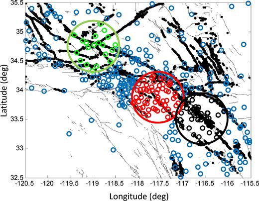
A location map with main faults (black) and seismic stations of the southern California seismic network (circles) used for the time period 2016 June 11–13. Green, red and black circles with 50 km diameter define three subarrays with 20 (green), 60 (red) and 103 (black) stations. The presented beamforming analysis is performed for a total of 375 subarrays with at least 15 stations.
The examined noise data are recorded during three consecutive days (2016 June 11–13), and analysed with time windows of half an hour for each beamforming output. We start with a basic pre-processing of the raw data, consisting of removing high-amplitude events within each 30 min window by clipping the amplitude at four times the raw noise standard deviation. After pre-processing, data recorded by 375 subarrays are beamformed for every 30 min window (with a 50 per cent time window overlap) over the 72 hr of the examined time. The analysis focuses on the vertical component of the broad-band seismometers to avoid the potential ambiguity between Rayleigh and Love waves in the phase velocity interpretation. The results provide a likelihood surface in the angle-velocity space (Fig. S1, Supporting Information), and the maximum value is used to determine the corresponding surface noise incident angle θ0 and velocity c0. Beamforming resolution is classically bounded by the array size through diffraction limits calculated in the far field at each frequency. However, adaptive beamforming significantly improves the resolution of the diffraction-limited beamformer by computing a maximum-likelihood type minimization between the data and model (Capon 1969; Jensen et al. 2011; Vandemeulebrouk et al.2013). The angle resolution of the adaptive beamformer output is around 10°, depending on frequency. High resolution is still linked to the size of the subarray, and is also strongly dependent on the SNR and the adequate match between the plane-wave propagation model and data. Similarly, the phase velocity resolution for one subarray is around 300 m s−1.
Fig. 2(a) displays the obtained collection of surface noise incident angles for a 30 min time window on June 11 at frequency 0.07 Hz, with an arrow pointing in the noise direction positioned at the centre of each subarray. As expected (Friedrich et al.1998; Gerstoft & Tanimoto 2007; Roux 2009), the ambient noise at 0.07 Hz clearly originates from the nearby Pacific Ocean with an average incident angle of 58° from the north (positive rotation clockwise). Similar analysis for 0.15 Hz (not shown) indicates again a dominant propagation from the Pacific with an average incident angle 46°. Fig. 2(b) shows the spatial variation of the obtained phase velocities for a selected 30 min time window. The phase velocities vary smoothly with relatively high and low values clustered in specific regions (e.g. around major faults and mountains). The variations may first appear surprising compared to the relatively uniform noise incident angle pattern in Fig. 2(a). However, the relative phase velocity variation Δc/c ∼ 10 per cent is in agreement with the relative angle fluctuation Δθ/θ, as expected from Snell's law for refracted rays.
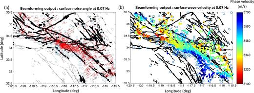
Results of the beamforming output maxima at 0.07 Hz for all subarrays obtained in a 30 min time window during 2016 June 11. (a) Propagation directions of noise-based surface waves (arrows positioned at the centre of each subarray) are clustered around 58°. (b) Phase velocities with spatial variations that correlate with major geological units in the study region.
Over the course of the three recording days, the standard deviation for the incident angle at 0.15 Hz is larger than at 0.07 Hz. This confirms that (1) the surface noise incident angle is sensitive to more complex structure at higher frequency, and (2) higher frequencies are more sensitive to small earthquakes that contaminate the incident angle measurement associated with pure ocean noise, which result in a degraded adaptive beamformer output (Fig. S2a, Supporting Information). To proceed with higher quality maps, beamforming results in every subarray for time windows having main direction outside an interval around the average incident angle plus or minus its standard deviation are rejected. The remaining beamforming output provide a large number of local phase velocities that cover southern California. The distribution of phase velocities is characterized by a dominant average peak with a frequency-dependent variance (Fig. S2b, Supporting Information).
When backprojected and averaged onto a 2-D map, the phase velocities over the three recording days reveal spatial variations (Figs 3a–c) that correlate with major geological units (Fig. 3d). Lower velocities are observed in places with deep sediments (e.g. Ventura and Los Angeles Basins, Coachella Valley and Salton Trough), while higher velocities are found around mountains (Peninsular Ranges Batholith and Transverse ranges) and in a region of the Mojave Desert with relatively deep Moho (Ozakin & Ben-Zion 2015). To transform the collection of local phase velocities into a velocity map sampled on a 2-D grid, we spatially average local phase velocities inside a 25 km diameter disc centred at each gridpoint. This spatial averaging is consistent with the fact that each beamforming output is the result of an array processing for stations within a 50 km disc. The standard deviation of the phase velocity maps in Figs 3(a)–(c) is as small as 2 per cent around 0.05 Hz and reaches a maximum value of 5 per cent at 0.15 Hz. Performing a similar averaging process on a 2-D grid provides a map for the noise incident angles (Fig. 4). The spatial distribution of the noise incident angle at low frequency exhibits a slow variation from 214° to 204° along a profile following the southern California coastline from south to north.
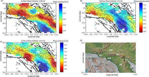
(a)–(c) Phase velocity maps obtained at discrete frequencies of 0.05, 0.1 and 0.15 Hz from the set of beamforming outputs during the three recording days. The results are obtained by averaging phase velocities derived as in Fig. 2(b) for 30 min time windows in time, and spatially smoothing the results on a 2-D grid with a 25 km filter. (d) A topographic map for southern California from the GMRT data set (Ryan et al.2009) with several geographic markers. VB = Ventura Basin, LAB = Los Angeles Basin, CV = Coachella Valley, ST = Salton Trough, MD = Mojave Desert, PR = Peninsular Ranges and TR = Transverse Ranges. The phase velocity maps at different frequencies are correlated with major geological structures and are in good agreement with results obtained with yearly averaged noise-correlation results.
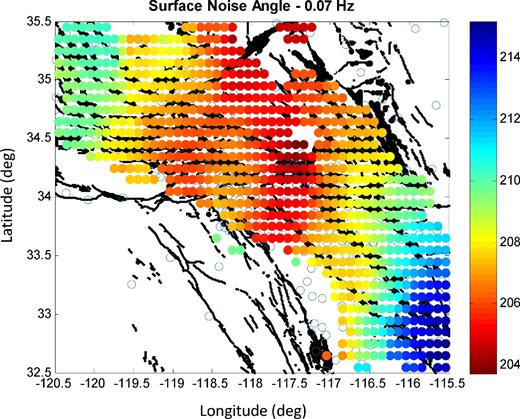
A map of noise incident angles obtained for Rayleigh surface waves at 0.07 Hz in a similar way as for the phase velocities in Fig. 3. The smooth changes of incident angles from south to north follow variations of the shoreline shape in southern California.
It would be useful to compare the final phase velocity maps obtained at different frequencies from beamforming (Figs 3a–c) with phase and group velocity maps obtained from ambient noise correlations that are typically produced from long time-averaged processing (Sabra et al.2005; Shapiro et al.2005; Yang et al.2008; Lin et al.2009; Barak et al.2015; Jin & Gaherty 2015; Zigone et al.2015). Unfortunately, most of the studies on phase velocities focused on the scale of the western U.S. continent with spatial resolution that does not allow for a quantitative comparison with the present regional work. We therefore simply note the good overall correlations between low- and high-velocity zones in our phase velocity maps with corresponding velocity zones in the above-mentioned noise-correlation studies, and the topographic map of Southern California (Fig. 3d).
3 DISCUSSION
The spatial resolution of phase velocity maps in Figs 3(a)–(c) should be interpreted with care. First, the adaptive beamforming output is associated with a ±300 m s−1 velocity main lobe around the maximum (Fig. S1, Supporting Information). This velocity resolution depends not solely on the number of wavelengths inside each subarray that is bounded by the 50 km size disc, but more on the match between the ambient noise data and the plane surface wave model. Second, the spatial averaging that permits to backproject the collections of sparse local phase velocities into a regular 2-D grid produces a spatial smoothing on a 25 km distance. Considering ocean-driven seismic noise at 0.1 Hz and seismic velocity of Rayleigh waves around 3 km s−1, the surface wave wavelength is 30 km. This distance defines the upper limit between neighbouring stations needed to avoid aliasing problems in the beamforming output. This means that beamforming over the examined frequency range data of the American USArray network (with interdistance stations on the order of 70 km) may lead to biased results, while the Japanese network Hi-net (with interdistance stations on the order of 20 km) is likely to be more appropriate.
Outside of time windows where the incoming seismic wavefield is dominated by local or teleseismic events, for which body and surface waves are mixed together, the adaptive beamforming process gives a stable and robust estimation of the local phase velocity independently of the directive or omnidirectional nature of the noise sources (and incident surface waves). In the case of directive incident noise, as in southern California where noise in the analysed frequency range comes from the Pacific ocean, local anisotropy may induce some bias in the phase velocity measurement. At other locations where ocean noise can have time variations over a large range of incident angles (e.g. in Japan), a measurement of local anisotropy could be extracted from beamforming results performed on a dense array.
As shown in Figs 3(a)–(c), the adaptive beamforming technique based on the ambient noise can provide surface wave properties. It is interesting to compare the array-based beamforming method to the two-point noise-correlation technique that was developed first in southern California over 10 yr ago, as both methods aim at providing surface wave tomography results. First, the main beamforming requirement is on the array design that should be dense enough to provide resolution without suffering from spatial aliasing. Therefore, beamforming applications to surface wave tomography requires large and dense arrays of seismometers, which is now a dominant trend at local, regional and continental scales. In contrast, the two-point noise-correlation process can be performed successfully with sparse distribution of sensors as long as spatial coherence survives the attenuation damping or the incoherent noise fluctuations. Second, beamforming is classically a frequency-domain process, while the two-point noise correlation is a time-domain broad-band processing. This implies that beamforming provides phase velocities, while noise correlation leads to group velocities. These differences make the two techniques complementary. We note, however, that an optimal application of noise-correlation requires omnidirectional ambient noise properties, which typically involves yearly averaged time-consuming processing. On the other hand, beamforming can give satisfactory results in a few hours to days only, which makes it advantageous when a rapid assessment of medium properties is needed.
The positive aspect that beamforming is not biased by directive incident noise, unlike the two-point noise correlations, may be balanced by the fact that beamforming requires a match between data-driven cross-spectral density matrix and surface wave propagation model. With increasing frequencies, the surface wave model may become complex since the wavelength becomes sensitive to lateral heterogeneities. For this reason, beamforming-based phase velocity maps of the type shown in Figs 3(a)–(c) are limited in southern California to frequencies below 0.2 Hz. However, data recorded by local arrays with very small instrument spacing (e.g. Ben-Zion et al.2015; Roux et al.2016) may be used to derive phase velocities and noise propagation directions associated with considerably higher frequencies. It is also worth mentioning that in terms of signal processing complexity, the beamforming match between data and model can be viewed as projection of the data into the model space. This algorithm is less involved (smaller number of steps and parameters) than the process that is classically performed from the set of two-point noise-correlation traveltimes, and is therefore less prone to have problems and artefacts. The derived phase velocities can be inverted with standard techniques for a shear wave velocity model. This may be the subject of a follow-up work.
Acknowledgements
We thank the operators of the southern California seismic network for recording and archiving the waveforms (SCECD 2013), Pieter-Ewald Share for help with downloading the data and Ramon Arrowsmith for help with generating Fig. 3(d). The paper benefitted from useful comments of two anonymous referees. ISTerre is part of Labex OSUG@2020. YBZ acknowledges support from the U.S. Department of Energy (award DE-SC0016520).
REFERENCES
SUPPORTING INFORMATION
Supplementary data are available at GJI online.
Figure S1. Normalized beamforming output for surface waves at 0.07 Hz, from 30 min of ambient noise recorded on 2016 June 11, performed on the red subarray with 60 stations in Fig. 1. Angles are measure with respect to the north, with positive rotation clockwise. The beamforming maximum (black dot) corresponds to a surface wave phase velocity of 3350 m s−1 and noise incident angle of 63°.
Figure S2. Normalized distributions of (a) incident angle and (b) phase velocity for the collection of all beamforming outputs at different frequencies for every 30 min time window and every subarray over the three recording days. The normalization is done for each frequency. The angle distribution spreads over frequencies above the first microseism peak (centred around 0.07 Hz), whereas the phase velocity distribution remains centred on its average.
Please note: Oxford University Press is not responsible for the content or functionality of any supporting materials supplied by the authors. Any queries (other than missing material) should be directed to the corresponding author for the paper.
