


Abstract
The Collaboratory for the Study of Earthquake Predictability was developed to prospectively test earthquake forecasts through reproducible and transparent experiments within a controlled environment. From January 2006 to December 2010, the Regional Earthquake Likelihood Models (RELM) Working Group developed and evaluated thirteen time-invariant prospective earthquake mainshock forecasts. The number, spatial and magnitude components of the forecasts were compared to the observed seismicity distribution using a set of likelihood-based consistency tests. In this RELM experiment update, we assess the long-term forecasting potential of the RELM forecasts. Additionally, we evaluate RELM forecast performance against the Uniform California Earthquake Rupture Forecast (UCERF2) and the National Seismic Hazard Mapping Project (NSHMP) forecasts, which are used for seismic hazard analysis for California. To test each forecast's long-term stability, we also evaluate each forecast from January 2006 to December 2015, which contains both five-year testing periods, and the 40-year period from January 1967 to December 2006. Multiple RELM forecasts, which passed the N-test during the retrospective (January 2006 to December 2010) period, overestimate the number of events from January 2011 to December 2015, although their forecasted spatial distributions are consistent with observed earthquakes. Both the UCERF2 and NSHMP forecasts pass all consistency tests for the two five-year periods; however, they tend to underestimate the number of observed earthquakes over the 40-year testing period. The smoothed seismicity model Helmstetter-et-al.Mainshock outperforms both United States Geological Survey (USGS) models during the second five-year experiment, and contains higher forecasted seismicity rates than the USGS models at multiple observed earthquake locations.
INTRODUCTION
Development and rigorous testing of earthquake forecasts is crucial for assessing their potential contribution to improving seismic hazard models. Seismic hazard assessment requires seismicity forecasts that can provide accurate future seismicity distributions over long periods of time. In 2000, the Regional Earthquake Likelihood Model (RELM) working group formed to refine the underlying seismicity models used in seismic hazard assessment in California as well as to improve the understanding of how earthquake occurrence can be characterized physically and statistically. To run forecast testing experiments, the group designed a testing centre, which was implemented by RELM's successor, the Collaboratory for the Study of Earthquake Predictability (CSEP; Jordan 2006). The CSEP testing centre was built upon prospective evaluation of seismicity forecasts against observed seismicity. Within the CSEP framework, described in the ‘CSEP testing centre framework’ section, the RELM working group established a set of consistency tests to evaluate each forecast in the RELM experiment against observed seismicity during a testing period (Schorlemmer et al.2007; Zechar et al.2010a), as well as a set of comparative tests to evaluate the performance of one forecast over another (Rhoades et al.2011). The testing suite provides an unbiased approach to learn about seismicity models’ strengths and weaknesses, indicating dimensions (e.g. space, magnitude) in which forecasts fail (Zechar et al.2013); a brief overview is given in the ‘Methods’ section.
Supported by the Southern California Earthquake Center (SCEC) and the United States Geological Survey (USGS), the RELM Working Group developed nineteen time-invariant earthquake forecasts for California (Field 2007, and references therein). In this suite were thirteen mainshock forecasts, that only forecast mainshocks as defined by the declustering approach of Reasenberg (1985) (described in Schorlemmer et al.2007), and six mainshock+aftershock forecasts, that include all earthquakes. In the RELM experiment, they tested all forecasts in the period January 2006 to December 2011, designing their forecast experiment to be truly prospective with all forecasts being finalized before the observation period had started.
During this time, two seismicity models were developed by the USGS: the seismicity model developed for the National Seismic Hazard Mapping Project (NSHMP; NSHMP 2008), and the second iteration of the Uniform California Earthquake Rupture Forecast (UCERF2; Field et al.2009) seismicity model. Both models were developed to become the basis for long-term seismic hazard analysis in California. A description of both models is given in the ‘UCERF2 and NSHMP models’ section. In contrast to most of the RELM models, both USGS models were developed primarily from geophysical data instead of historical seismicity. Furthermore, the combination of input models composing the USGS models—fault, deformation, earthquake rate and for UCERF2, probability of an earthquake occurring within a given time interval—was based on expert opinion, whereas the RELM models were algorithm-based. The UCERF2 and NSHMP five-year forecasts were not evaluated during the initial RELM mainshock experiment.
To evaluate both USGS models and investigate the stability of the results of the RELM forecast tests, we conducted an update to the initial five-year forecasting experiment. In the current study, we retrospectively evaluate the USGS and RELM forecasts during the observation period of the original RELM experiment (Schorlemmer et al.2010; Zechar et al.2010b), and prospectively test the forecasts from January 2011 to December 2015. We also test the forecasts over the ten-year period containing both five-year periods (January 2006 to December 2015). To confirm that the forecasts are consistent with earthquake data used in their calibration, we test the forecasts over the January 1967 to December 2006 40-year evaluation period. We define these evaluation periods as the time intervals from which earthquake data are used to evaluate model consistency with observed seismicity. Additionally, we investigate the limits of forecast performance information that can be obtained from current CSEP forecast evaluation methods.
In this paper, after detailing the RELM and USGS seismicity models under study, we describe the CSEP testing centre framework and experiment design. We then introduce our consistency and comparative testing methods, including the testing suite from the RELM Working Group as well as residual methods. The evaluation results follow, showing that both USGS forecasts pass all consistency tests for both five-year intervals. The forecast developed by Helmstetter et al. (2007) overpredicts the total number of earthquakes during the second five-year interval, despite performing the best among the RELM forecasts in the original experiment. However, during all other evaluation periods, both USGS forecasts can be rejected in favour of this top-performing RELM forecast.
UCERF2 and NSHMP models
The UCERF2 (Fig. 1) and NSHMP forecasts were developed by the Working Group on California Earthquake Probabilities (WGCEP). Both forecast models are based on a combination of geophysical (strain rate) and historical seismicity data (Field et al.2009). Ruptures on faults with sufficient palaeoseismic rupture constraints and slip-rate data are hypothesized to occur within segments of those faults, each of which is assigned a stress-renewal recurrence model (WGCEP 1995). Regions with well-constrained slip rates but inadequate spatiotemporal seismicity data to assign stress-renewal probabilities are modelled as characteristic full-fault ruptures. Rupture magnitudes are generated from a Gaussian frequency-magnitude distribution and allow for multiple faults to rupture simultaneously in one large event. Where slip-rate data are incomplete or unable to be assigned to specific faults, seismicity rates are based on strain rates where geodetic data are available; otherwise, seismicity rates are derived from smoothed historical seismicity (Field et al.2009). Unlike the RELM models, which were declustered using the Reasenberg algorithm (Reasenberg 1985), both USGS models were declustered using the Gardner and Knopoff algorithm (Gardner & Knopoff 1974).
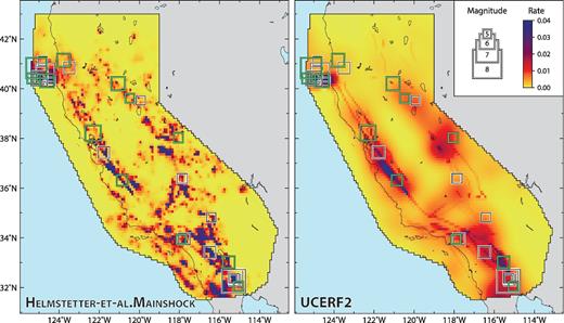
Five-year seismicity forecasts for the Helmstetter-et-al.Mainshock and UCERF2 forecasts. Purple and dark red regions have elevated seismicity rates, whereas seismicity is lower within yellow areas. Seismicity rates are considered time-invariant, that is, they are not updated as new earthquake data become available and the same forecasts are used for both five-year experiments. Black and green squares indicate the locations of observed earthquakes occurring during the five-year retrospective and prospective experiments, respectively.
Throughout the entire testing region, the NSHMP forecast assumes a Poisson earthquake distribution over time. Earthquakes are assumed randomly distributed over time, given a forecasted seismicity rate. In the UCERF2 forecast, earthquake probabilities do not follow a Poisson distribution within the fault segments where stress renewal probabilities can be assigned. Rather, they are based on elastic rebound theory (Reid 1911). In these subregions, earthquake probabilities are conditioned to the stress state at the time of the last rupture. According to the ‘earthquake cycle’ assumption, large earthquakes are assumed to have released most or all accumulated stress on a fault segment, greatly lowering the probability of a future earthquake immediately following the event (Reid 1911). Over time, aseismic stress accumulation gradually increases the probability of an earthquake within a future time interval. Because fault zones with assigned stress renewal models comprise only a small fraction of the total testing region, the NSHMP and UCERF2 forecasts produce identical seismicity rates in most areas.
CSEP testing centre framework
The purpose of CSEP is to evaluate the consistency of seismicity models with observed seismicity and compare performances of forecast model pairs. Forecasts are tested against observed seismicity using a set of likelihood-based consistency tests (Schorlemmer et al.2007; Zechar et al.2010a) and their relative performance to each other is tested to determine the best performing model using a set of comparative tests (Rhoades et al.2011). In contrast, previous earthquake forecasting experiments merely compared one forecast model against a null hypothesis, as described by Schorlemmer & Gerstenberger (2007).
Each CSEP testing centre hosts forecasting experiments in designated testing regions. In an experiment, the testing region is divided into spatiomagnitude bins based on longitude, latitude and magnitude increments. The period during which forecasts are evaluated can vary from minutes to decades; an evaluation period is designated for each forecasting experiment. Furthermore, all forecasts in an experiment must originate from the same testing class, which are forecasts in the case of the RELM experiment. When submitting rate-based forecasts to a CSEP testing centre, modellers must provide expected numbers of earthquakes in each spatiomagnitude bin during the evaluation period.
The CSEP testing centre is capable of testing forecasts both retrospectively and prospectively. In prospective tests, forecasts are made for future periods and are tested exclusively against observations occurring after the forecast was issued. Modellers can no longer modify their forecasts based on new seismic or geophysical data. This ensures that no prior knowledge of the observations is used for testing the forecasts. Prospective testing should not be confused with the so-called ‘pseudo-prospective’ testing in which forecasts are tested during a ‘pseudo’ future period, but created entirely from data before it. In this case, the model cannot incorporate any data from the testing period (like in prospective testing). However, it cannot be ruled out that knowledge of the observations and their features has been consciously or unconsciously included in the model, hereby creating a bias. Under such conditions, the true forecasting power of a model cannot be estimated and the test cannot be considered rigorous. In contrast to these two approaches, forecasts are retrospectively tested against known data from the past. Such tests are important in identifying forecast inconsistencies, e.g. a forecast should pass a test against data from which it was created, which can be considered a sanity check. However, retrospective testing can under no circumstance replace prospective testing if the forecasting power of models is under scrutiny (Werner et al.2010).
The RELM experiment prompted a series of subsequent forecasting experiments and the establishment of multiple CSEP testing centres throughout the world. In November 2009, the Japan CSEP testing centre began a prospective forecasting experiment covering three regions in Japan (Tsuruoka et al.2012). Modellers submitted 91 forecasts to be evaluated over one-day, three-month, one-year and three-year observation periods. Initial results suggested that time-dependent forecasts such as the Epidemic Type Aftershock Sequence (ETAS) seismicity outperform smoothed seismicity forecasts when evaluated over short time intervals (one-day to three-year). Following the 2011 September 4 earthquake in Canterbury, New Zealand, a group of modellers retrospectively tested nine seismicity-based and three physics-based forecasts (one-day to one-year evaluation periods). During retrospective evaluation, the physics-based models outperformed the statistics-based models during the one-year evaluation period. Forecasting experiment results in Italy for five- and ten-year evaluation periods (Werner et al.2010) challenged the assumption that declustered earthquakes follow a Poisson distribution. The smoothed seismicity-based forecast developed by Eberhard et al. (2012) for the western Pacific region was a prototype for future global forecasts, including the Global Earthquake Rate (GEAR) forecast (Bird et al.2015). Today, hundreds of earthquake forecasts are undergoing prospective evaluation in the CSEP testing centres.
To prevent modellers from introducing biases into forecast models, earthquake data used to test forecasts are provided by an authoritative and independent source. Such a data source is defined as part of each CSEP experiment. Furthermore, each forecasting experiment is designed to be transparent and reproducible (Zechar et al.2010b). Computer code used to run CSEP experiments is documented and can be provided to users to conduct them independently. To prevent varying test results as a consequence of modified earthquake catalogues, the testing centres retain the original earthquake data used in each experiment. This also allows CSEP testing centres to rerun any previous experiment.
Experiment design
Most RELM forecasts are based on smoothed historical seismicity, although some forecasts incorporated geodetic and/or geologic data. Detailed descriptions of input data for each model are given in Field (2007) and Schorlemmer et al. (2010); a brief summary of input data for each mainshock model, along with corresponding references, is given in Table 1. Experiment names, durations, and retrospective or prospective designations are given in Table 2; we will henceforth refer to experiments by their corresponding names.
Summary of input data used in developing RELM seismicity models. Most models were based upon historical seismicity catalogues; however, the b-values, magnitude thresholds and catalogue duration times vary considerably. The five-year forecasts were developed from the seismicity models by calculating seismicity rates over a five-year interval. RELM model names remain unchanged from the original experiment (Schorlemmer et al.2010).
| RELM mainshock model name | Regional fit | Input data |
|---|---|---|
| Ebel-et-al.Mainshock.Corrected | Active fault zones | Average rate of M ≥ 5 declustered earthquakes from the period 1932–2004 (Ebel et al.2007) |
| Helmstetter-et-al.Mainshock | Full CA | Smoothed M ≥ 2 earthquakes since 1981, optimized smoothing kernel, spatially varying magnitude of completeness (Helmstetter et al.2007) |
| Holliday-et-al.PI | High-seismicity zones | Regions with strongly fluctuating seismicity rates expected to contain large earthquakes (Holliday et al.2007) |
| Kagan-et-al.Mainshock | Southern CA | Smoothed seismicity since 1800, accounts for large rupture areas (Kagan et al.2007) |
| Shen-et-al.Mainshock | Southern CA | Earthquake rate is proportional to horizontal maximum shear strain rate (Shen et al.2007) |
| Ward.Combo81 | Southern CA | Average of Ward.Geodetic81, Ward.Geologic81, and Ward.Simulation forecasts (Ward 2007) |
| Ward.Geodetic81 | Southern CA | Seismicity rates derived from strain rates, magnitudes forecasted with truncated Gutenberg-Richter distribution (M = 8.1) (Ward 2007) |
| Ward.Geodetic85 | Southern CA | Same as Ward.Geodetic81 forecast, with M = 8.5 (Ward 2007) |
| Ward.Geologic81 | Southern CA | Smoothed geological moment rate density from mapped fault slip rates (Ward 2007) |
| Ward.Seismic81 | Southern CA | Smoothed seismicity since 1850 (Ward 2007) |
| Ward.Simulation | Southern CA | Simulations of velocity-weakening friction on fixed fault network (Ward 2007) |
| Wiemer-Schorlemmer.ALM | Full CA | Spatially varying a- and b-values influence rate of larger earthquakes (Wiemer & Schorlemmer 2007) |
List of evaluation experiments. The experiment names start with the length of the experiment period (i.e. 5year), while pro and retro correspond to prospective and retrospective experiments, respectively. The designation of prospective or retrospective in the experiment name is based on the type of evaluation of the two USGS forecasts.
| Experiment name | Experiment period | RELM forecasts | USGS forecasts |
|---|---|---|---|
| 5year.retro | 2006–2011 | Prospective | Retrospective |
| 5year.pro | 2011–2016 | Prospective | Prospective |
| 10year.retro | 2006–2016 | Prospective | Retrospective |
| 40year.retro | 1967–2007 | Retrospective | Retrospective |
The testing region included the area within California and a zone of one degree surrounding it, to include earthquakes outside California that can cause hazardous shaking in the state. The testing region is divided into spatial-magnitude bins, with 0.1° × 0.1° spatial cells and 0.1-increment magnitude bins (4.95 ≤ M < 5.05, 5.05 ≤ M < 5.15, etc.). The maximum magnitude bin, M ≥ 8.95, contained no upper magnitude limit. Within each bin, the modellers provided expected numbers of earthquakes, which were assumed to follow a Poisson distribution (Zechar et al.2013). Some RELM forecasts only partially covered the RELM testing region, with several only covering southern California (Schorlemmer et al.2010).
We used the observation earthquake catalogues from the Advanced National Seismic System (ANSS) database as generated by the CSEP testing centre in California. In the case of mainshock forecast evaluation, we declustered the observation earthquake catalogue using the algorithm by Reasenberg (1985), using algorithm parameters standard for California (Schorlemmer & Gerstenberger 2007). The choice of declustering algorithm and parameters was agreed upon by testers and modellers contributing to the original RELM experiment.
Forecast evaluation methods
Likelihood consistency tests
The likelihood consistency test suite evaluates the consistency of forecasted and observed seismicity patterns during an evaluation period. Each test is based on the likelihood of an observed seismicity distribution, given forecasted seismicity rates.
Likelihood test (L-test)
A forecast's log-likelihood score, based on the Poisson distribution, is a metric used to evaluate the consistency of a forecast with observed earthquakes: the greater the log-likelihood, the greater the consistency. A greater consistency indicates a higher probability of the forecast producing a seismicity distribution similar to observed seismicity and thus, greater faith in the model's ability to forecast earthquakes. In the likelihood test, or L-test, multiple synthetic earthquake catalogues are simulated from the forecast, representing different possible catalogues according to the forecast (Schorlemmer et al.2007). Log-likelihoods from these synthetic catalogues are then compared to the log-likelihood computed from observed seismicity. The L-test is two-tailed because this log-likelihood is inconsistent with observed seismicity if it falls within either tail of the simulated log-likelihood distribution. The same is true for all other consistency tests. The distribution tails are defined at greater than 0.975 or less than 0.025 of the distribution, that is, a 0.05 chance of a Type I error. In the original RELM experiment, the L-test was one-tailed, under the assumption that a forecast should not be rejected for high performance (i.e. high likelihood scores).
A forecast's consistency with observed seismicity can be decomposed into three dimensions: number of earthquakes, their magnitude and their spatial distribution. From these components, further tests of the CSEP likelihood test suite are derived (Zechar et al.2010a).
Number test (N-test)
The N-test evaluates whether the observed total number of earthquakes within a time interval is consistent with the forecasted total number. The total number of forecasted earthquakes is defined as the sum of earthquakes forecasted over all spatiomagnitude bins (Schorlemmer et al.2007; Zechar et al.2010b). As the test includes no information regarding the spatial and magnitude seismicity distribution, it can be conducted without generating a distribution of earthquakes simulated from the forecast, as described above for the L-test.
Earthquake rates in each spatiomagnitude bin are considered to follow the Poisson distribution independently of each other. As such, the total forecasted earthquake number is considered to also follow a Poisson distribution. The mean, the only parameter for the Poisson distribution, is likewise defined as the total forecasted number of events. Forecasts can be rejected either for over- or underpredicting total numbers of observed earthquakes.
Magnitude test (M-test), spatial test (S-test), and conditional likelihood test (CL-test)
The M- and S-tests are based on the L-test, the result of which depends primarily upon the total number of observed earthquakes. In most spatiomagnitude bins, the forecasted number of earthquakes is close to zero due to the bins’ small spatiomagnitude volume. This causes target bins, or bins containing at least one observed earthquake, to decrease the overall log-likelihood considerably more than bins containing zero earthquakes. Therefore, forecasts nearly always fail the L-test if they fail the N-test, and the L-test fails to provide additional information. Despite the lack of new information that the L-test provides, we include the results in this study to remain consistent with the first phase of the RELM experiment.
The CL-test was developed to isolate information regarding the consistency of the forecasted and observed spatial and magnitude distributions (Zechar et al.2010a; Werner et al.2011). In the CL-test, the number of forecasted earthquakes is normalized such that it is equal to the observed number, removing the influence of the number of forecasted events on the corresponding log-likelihoods. Apart from this normalization, the CL-test procedure and purpose is identical to that of the L-test. Because the CL-test does not provide any additional information beyond the M- and S-tests, we do not include these test results.
We test the consistency of the forecasted earthquake distribution in the magnitude and spatial domains, to determine if the forecasted magnitude and spatial distributions are consistent with those of the observed seismicity. The M- and S-tests, evaluating forecasted magnitude and spatial distributions, respectively, are directly derived from the CL-test (Zechar et al.2010b). In these tests, the spatial and magnitude distribution consistencies between forecasted and observed seismicity are respectively isolated. For the S-test, we consider forecasted earthquake numbers within spatial bins, or the sum of forecasts over all corresponding magnitude bins for a particular latitude-longitude interval. In the case of the M-test, we consider the analogous sum over all spatial bins within a magnitude level. As with the CL-test, the total number of forecasted earthquakes is first normalized to equal the observed earthquake count.
Likelihood test assumptions
Two central assumptions made in these tests limit how effectively forecasted and observed seismicity can be characterized and compared. The assumption that binwise seismicity forecasts are independent of each other places arbitrarily defined constraints on boundaries in the forecast grid, which have no physical interpretation (Zechar et al.2010b; Schneider et al.2014). The second assumption is that forecasted earthquake rates are considered to follow the Poisson distribution within spatiomagnitude bins. The Poisson assumption has been under debate for years in the seismological community (Gardner & Knopoff 1974; Harte 2015). The Poisson distribution is relatively simple to apply, only requiring one parameter. However, Harte (2015) shows that self-exciting point-process models, where the recent occurrence of earthquakes increases the probability of future earthquakes, do not produce Poisson earthquake counts in discrete spatiotemporal bins. Lombardi & Marzocchi (2010) suggests that seismicity during short time intervals does not follow a Poisson distribution, and Kagan (2010) states that the Poisson hypothesis cannot be applied to undeclustered seismicity. Schorlemmer et al. (2010) found that seismicity rates in the RELM testing region in the period 1932–2005 were better represented by the negative binomial distribution than the Poisson distribution. However, the best-fit negative binomial distribution fit the observed mainshocks only marginally better than the best-fit Poisson distribution. Schneider et al. (2014) found similarly negligible differences in N-test results between both distributions for three-month California earthquake forecasts. Because of the small difference reported between the two distributions, to remain consistent with the first five-year RELM experiment procedure, and because forecasted seismicity rates are given as Poisson rates, we retain the Poisson assumption for all likelihood tests.
Concentration plots
Concentration plots provide a general assessment of a seismicity model's consistency with observed seismicity, as well as indicate whether the model is over-smoothed or too ‘localized’ (Helmstetter et al.2007). For a given evaluation period, the cumulative distributions of forecasted and observed earthquake numbers are plotted as a function of the bin-wise forecasted seismicity. If there is no significant deviation between the two distributions, one considers the model consistent with observed seismicity. If the forecasted distribution is shifted to the left of the observed distribution, the model is too smooth; that is, observed earthquakes occur in regions with higher, more concentrated seismicity. If the opposite is true, the model is too localized, such that more earthquakes occur in zones with low forecasted seismicity.
Forecast comparison and point process residuals
The comparison tests compare two forecasted seismicity distributions’ consistencies with observed seismicity. These tests are based on a hypothesis testing framework, and result in a decision on whether to reject one forecast in favour of another. Point process residuals provide a visualization of local spatial variations in forecast performance.
T-test and W-test
The relative performance of two forecasts may be evaluated by measuring the information gain score at each observed earthquake location of one forecast over another. The information gain score is a test metric that indicates the relative performance of two forecasts at an observed earthquake location (Rhoades et al.2011). Applying the Student's paired t-test, we consider the null hypothesis that the two forecasts perform equally well, and the alternate hypothesis that one forecast can be rejected in favour of the other. If the null hypothesis is true, the mean information gain is equivalent to the scaled difference in forecasted earthquake numbers between the two forecasts. If one forecast significantly outperforms the other, then the mean information gain differs from this scaled difference.
Although information gain scores at observed earthquake locations are often not normally distributed (Eberhard et al.2012; Schneider et al.2014), the central limit theorem proves that their distribution approaches a normal distribution as the number of scores approaches infinity. However, the M ≥ 4.95 threshold of the RELM and USGS forecasts limits the number of earthquakes observed during a five-year testing interval. In the case that the information gain scores are not normally distributed, the non-parametric W-test is preferred. This tests the median information gain per earthquake rather than the mean, only requiring that the information gain distribution is symmetric. The W-test becomes less powerful as the number of observed earthquakes decreases and is incapable of rejecting a forecast with fewer than five events at the 0.05 significance level (Rhoades et al.2011). Therefore, the W-test result should be corroborated by the T-test result to favour one forecast over another with statistical significance.
In the case that the information gain distribution is neither symmetric nor normally distributed, the T- and W-tests cannot provide informative comparisons of the two forecasts. Although we test all forecast pairs, T- and W-test results from forecast pairs with insufficient numbers of observed earthquakes are uninformative, and are not reported in the ‘Results’ section. The numbers of observed earthquakes in each forecast region during each testing period are given in Table 3. During the 5year.pro experiment, numerous forecasts had too few observed earthquakes to successfully apply either test.
Number of observed earthquakes within the forecast coverage areas, for each experiment.
| Forecast | 5year.retro | 5year.pro | 10year.retro | 40year.retro |
|---|---|---|---|---|
| UCERF2 | 17 | 12 | 29 | 179 |
| NSHMP | 17 | 12 | 29 | 179 |
| Ebel-et-al.Mainshock.Corrected | 17 | 11 | 28 | 179 |
| Helmstetter-et-al.Mainshock | 17 | 12 | 29 | 179 |
| Holliday-et-al.PI | 13 | 3 | 16 | 68 |
| Kagan-et-al.Mainshock | 11 | 4 | 15 | 89 |
| Shen-et-al.Mainshock | 11 | 4 | 15 | 87 |
| Ward.Combo81 | 9 | 3 | 12 | 71 |
| Ward.Geodetic81 | 9 | 3 | 12 | 71 |
| Ward.Geodetic85 | 9 | 3 | 12 | 71 |
| Ward.Geologic81 | 9 | 3 | 12 | 71 |
| Ward.Seismic81 | 9 | 3 | 12 | 71 |
| Ward.Simulation | 9 | 3 | 12 | 71 |
| Wiemer-Schorlemmer.ALM | 17 | 12 | 29 | 179 |
Deviance residuals
The CSEP consistency and comparative tests do not capture localized spatial variations between forecasted and observed seismicity distributions. Residuals scores from the point process modelling literature (Lawson 1993; Baddeley et al.2005; Clements et al.2011) are well-suited to resolve this particular issue. Forecasts can be represented as space-time point process models, where binwise forecasts are represented as infinitesimal seismicity rates at specific locations. By representing a forecast in such a way, one can locate specific areas where a forecast performs well or poorly through the use of point process residual methods (Clements et al.2011; Schneider et al.2014). An advantage to this representation is that no assumptions regarding binwise seismicity independence and Poisson seismicity within bins are required.
Deviance residuals are point process residual metrics which can be used to highlight differences in performance between two forecasts in spatial bins (Clements et al.2011; Schneider et al.2014). Within bins containing highly positive or negative deviance residuals, one forecast considerably outperforms the other in forecasting the observed seismicity. Therefore, deviance residuals can highlight areas of relative strength or weakness in each forecast as compared to another, which may be masked by the aforementioned hypothesis testing methods. This enables us to track how the presence of particular model features affects forecast performance, and how this varies over space. Clements et al. (2011) evaluated the mainshock+aftershock seismicity models developed by Helmstetter et al. (2007), Shen et al. (2007) and Kagan et al. (2007) during the evaluation period of the original RELM experiment. They found that the Helmstetter model outperformed the other two models within the Imperial earthquake cluster and the earthquake cluster just north of the California-Mexico border (lon ≈ 116.0°W and lat ≈ 32.7°N).
Residual scores can identify regions where the forecasted seismicity rate should be adjusted. Although deviance residual scores visualize spatiotemporal differences in forecast performance, they do not provide any significance information. Because deviance residuals lack a notion of statistical significance, they cannot yet be used to reject forecast models.
RESULTS
Observed earthquakes
In the entire testing region, seventeen M ≥ 4.95 mainshocks occurred during the 5year.retro experiment, while twelve mainshocks occurred during the 5year.pro experiment. The observed earthquakes during the 5year.retro experiment include two large mainshocks: the 2010 January 10 M6.5 earthquake offshore from Cape Mendocino, and the 2010 April 4 M7.2 El Mayor Cucapah earthquake in Baja California. During the 5year.pro experiment, an M6.8 earthquake occurred on 2014 March 10 in the vicinity of the previous M6.5 event. A total of 29 mainshocks occurred during the 10year.retro experiment, while 179 events were observed during the 40year.retro experiment.
Likelihood scores at earthquake locations
Table 4 displays log-likelihoods at each observed earthquake location for the 5year.retro and 5year.pro experiments. UCERF2 has the lowest log-likelihoods for nine earthquakes, due to lower forecasted earthquake numbers compared to the RELM forecasts. The best performing forecast from the original RELM experiment, Helmstetter-et-al.Mainshock, possesses the highest log-likelihoods for five events. Holliday.PI and Wiemer-Schorlemmer.ALM exceed this result with six and eight maximum log-likelihoods, respectively. Wiemer-Schorlemmer.ALM is the most spatially heterogeneous forecast, with elevated seismicity rates concentrated in small regions. In addition to possessing the greatest number of maximum log-likelihoods (eight), this forecast also contains the most minimum log-likelihoods (eleven). Additionally, the forecast's log-likelihood for the 2014 March 10 offshore M6.8 earthquake is nearly twice as negative as the competing forecasts’ scores, as well as the minimum log-likelihood for all forecasts and observed earthquake locations. The UCERF2 and NSHMP forecasts contain the highest log-likelihood at the location of the El Mayor Cucapah earthquake; Ward.Simulation contains the lowest score.
Log-likelihood scores at observed earthquake locations during the 10year.retro experiment. Cells with light grey shading indicate the forecasts with the highest log-likelihood; cells with dark grey shading indicate the forecasts with the lowest scores. The numbers 1–14 along the top row correspond to the forecast models: (1) UCERF2, (2) NSHMP, (3) Ebel-et-al.Mainshock.Corrected, (4) Helmstetter-et-al.Mainshock, (5) Holliday-et-al.PI, (6) Kagan-et-al.Mainshock, (7) Shen-et-al.Mainshock, (8) Ward.Combo81, (9) Ward.Geodetic81, (10) Ward.Geodetic85, (11) Ward.Geologic81, (12) Ward.Seismic81, (13) Ward.Simulation, and (14) Wiemer-Schorlemmer.ALM.
 |
|
Log-likelihood scores at observed earthquake locations during the 10year.retro experiment. Cells with light grey shading indicate the forecasts with the highest log-likelihood; cells with dark grey shading indicate the forecasts with the lowest scores. The numbers 1–14 along the top row correspond to the forecast models: (1) UCERF2, (2) NSHMP, (3) Ebel-et-al.Mainshock.Corrected, (4) Helmstetter-et-al.Mainshock, (5) Holliday-et-al.PI, (6) Kagan-et-al.Mainshock, (7) Shen-et-al.Mainshock, (8) Ward.Combo81, (9) Ward.Geodetic81, (10) Ward.Geodetic85, (11) Ward.Geologic81, (12) Ward.Seismic81, (13) Ward.Simulation, and (14) Wiemer-Schorlemmer.ALM.
|
|
Consistency tests
Likelihood tests
N-test and L-test:
Fig. 2 displays N-test results for each forecast and experiment. Eleven RELM forecasts overpredict the number of events in the 5year.pro experiment; four also overpredict during the 5year.retro period. Helmstetter-et-al.Mainshock fails the N-test during the 5year.pro and 10year.retro experiments due to overprediction. However, the forecasted number of events during the 40year.retro experiments are consistent with observed event numbers. The USGS forecasts, by contrast, pass the N-test for all experiments except the 40year.retro experiment when their total forecasted earthquake numbers are below those of most RELM forecasts. During the 40year.retro experiment, both USGS forecasts underpredict the number of observed earthquakes. The 40year.retro experiment functions as a ‘sanity check’, evaluating forecasts with those observations used to calibrate the underlying seismicity models. Therefore, the USGS forecast performances indicate that a five-year evaluation period may be insufficient to assess a forecast's long-term reliability. Other possible explanations include that background seismicity and/or seismicity rates along known, active faults were underestimated.
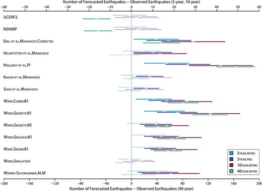
N-test results for the USGS and RELM forecasts. The difference between the total forecasted earthquake number and the total number of observed earthquakes is labelled by the horizontal axes, with scaling adjustments for the 40year.retro experiment. The horizontal lines represent the confidence intervals, within the 0.05 significance level, for each forecast and experiment. If this range contains zero, the forecasted number of earthquakes is consistent with the observed number, and passes the N-test (denoted by thin lines). If the minimum difference within this range exceeds zero, the forecast overpredicts; if the maximum difference falls below zero, the forecast underpredicts during the experiment. In both cases, the forecast fails the N-test for that particular experiment (denoted by thick lines). Colours distinguish between experiments (see Table 2 for explanation of experiment durations).
As described in the ‘Likelihood consistency tests’ subsection of the ‘Forecast evaluation methods’ section, the L-test results depend primarily upon the N-test results. That is, over- or underprediction resulted in forecasts failing the L-test as well as the N-test.
M-test and S-test:
Fig. 3 displays S-test results for each forecast and experiment. The USGS forecasts pass the S-test for all experiments except the 40year.retro, while Helmstetter-et-al.Mainshock passes the S-test for all four experiments. The difference in performance between the two forecasts can be attributed to two factors: an increased number of observed earthquakes in ‘background’ regions (away from major faults) rather than within large fault zones, and underestimated seismicity rates where observed earthquakes occurred along major faults for the USGS forecasts.
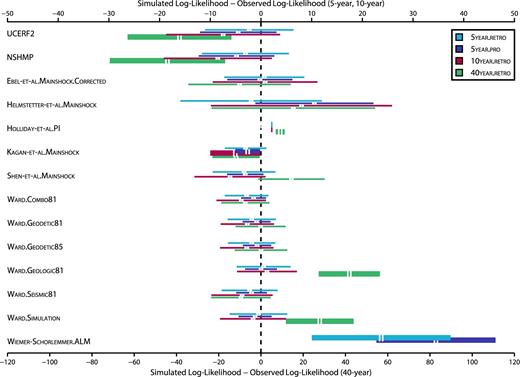
S-test results for the USGS and RELM forecasts. The differences between the simulated log-likelihoods and the observed log-likelihood are labelled on the horizontal axes, with scaling adjustments for the 40year.retro experiment. The horizontal lines represent the confidence intervals, within the 0.05 significance level, for each forecast and experiment. If this range contains a log-likelihood difference of zero, the forecasted log-likelihoods are consistent with the observed, and the forecast passes the S-test (denoted by thin lines). If the minimum difference within this range does not contain zero, the forecast fails the S-test for that particular experiment, denoted by thick lines. Colours distinguish between experiments (see Table 2 for explanation of experiment durations). Due to anomalously large likelihood differences, S-test results for Wiemer-Schorlemmer.ALM during the 10year.retro and 40year.retro experiments are not displayed. The range of log-likelihoods for the Holliday-et-al.PI forecast is lower than for the other forecasts due to relatively homogeneous forecasted seismicity rates and use of a small fraction of the RELM testing region.
Holliday.PI and Kagan.Mainshock fail the S-test for all experiments except 5year.pro and 5year.retro, respectively. Wiemer-Schorlemmer.ALM fails the S-test for all four experiments. For all forecasts except Holliday.PI and Kagan.Mainshock, the S-test results are the same between the 5year.retro and 5year.pro experiments.
With the exception of the Ward.Simulation model during the 10year.retro and 40year.retro experiments, all forecasts pass the M-test for all experiments. The lack of variation in the M-test results can be attributed to the similar Gutenberg-Richter distributions and parameters used to model forecasted earthquake magnitudes for the USGS and most RELM models.
Concentration plots
Concentration plots for UCERF2 and Helmstetter-et-al.Mainshock are shown in Fig. 4 for the 40year.retro experiment. There is visible deviation between the observed and forecasted seismicity distributions for UCERF2, which also failed the 40year.retro S-test. The observed distribution is shifted to the right of the forecasted distribution, suggesting that UCERF2 is over-smoothed. Although the distributions for Helmstetter-et-al.Mainshock appear more consistent (as would be expected from S-test results), the model is not smooth enough within high-seismicity zones, which fail to contain all observed earthquakes. Although there are only two years of overlap between the 40year.retro and 5year.retro experiments, the difference in the number of minimum log-likelihood scores at observed earthquake locations (Table 4) supports that Helmstetter-et-al.Mainshock tends to produce more reliable forecasts over long periods than UCERF2.
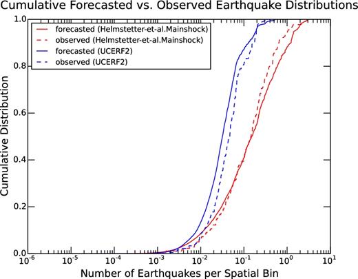
Concentration plots for the 40year.retro experiment, showing the cumulative forecasted versus observed seismicity distribution for UCERF2 (blue curves) and Helmstetter-et-al.Mainshock (red curves). For UCERF2, the observed distribution is shifted slightly to the right of the forecasted distribution, suggesting that the model is oversmoothed. The opposite is true for Helmstetter-et-al.Mainshock as forecasted earthquake numbers increase, suggesting that within high-seismicity zones, the model is not smooth enough.
Comparison tests and metrics
T-test and W-test
The T- and W-tests indicate whether or not the RELM and NSHMP forecasts can be rejected in favour of UCERF2, the baseline forecast considered. Fig. 5 displays results from both tests comparing UCERF2 with all other forecasts. For all experiments except 5year.pro, UCERF2 can be rejected in favour of Helmstetter-et-al.Mainshock. That is, Helmstetter-et-al.Mainshock has a statistically significant positive information gain over UCERF2. Additionally, most RELM forecasts can be rejected in favour of UCERF2 for the 40year.retro experiment.
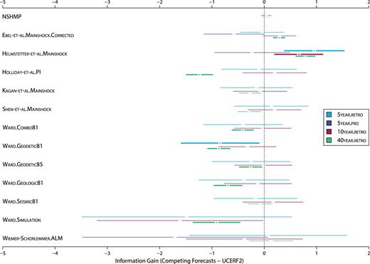
T- and W-test results, comparing UCERF2 against NSHMP and the RELM forecasts. The horizontal axis displays the information gain of each competing forecast over UCERF2, that is, positive information gain indicates that the competing forecast outperforms UCERF2. The horizontal lines show the confidence interval, within the 0.05 significance level, of competing forecasts. The points at the centre show the information gain point estimates. If the minimum information gain exceeds zero and is corroborated by W-test results, UCERF2 can be rejected in favour of the competing forecast. If the maximum information gain is below zero (and corroborated by the W-test), then the competing forecast can be rejected in favour of UCERF2. Thick lines indicate when one forecast can be rejected in favour of another; thin lines indicate no significant difference between forecast performances. If the forecasts contained fewer than five observed events during an experiments (see Table 3), this T- and W-test result was not reported.
During the 5year.pro experiment, twelve earthquakes occur in the RELM testing region, but only the earthquakes within overlapping forecast areas are included in the tests. Therefore, the statistical power of the T- and W-tests is dramatically reduced, particularly in cases involving RELM forecasts that include only southern California. Holliday.PI, which covers the least area in the RELM testing region, contains only three observed earthquakes during this second five-year experiment. Therefore, the T- and W-test results are uninformative for this forecast during the 5year.pro experiment (see the ‘Forecast comparison and point process residuals’ section for further explanation), and thus not plotted in Fig. 5.
Deviance residuals
We calculated deviance residuals, displayed in Fig. 6, to directly compare the UCERF2 and Helmstetter-et-al.Mainshock forecasts. Seismicity rates forecasted by Helmstetter-et-al.Mainshock exceed those forecasted by UCERF2 in several localized regions, some of which had earthquakes. The earthquake swarm near Cape Mendocino, including an M6.5 mainshock, occurred where Helmstetter-et-al.mainshock forecasted higher seismicity rates. This improved the forecast's performance during the first five-year RELM experiment. However, the M7.2 El Mayor mainshock occurred just outside of the southern zone with elevated seismicity rates, resulting in a lower log-likelihood for Helmstetter-et-al.Mainshock than for UCERF2 (Table 4), despite UCERF2 being rejected in favour of Helmstetter-et-al.Mainshock by the T-test (Fig. 5).
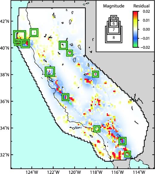
Deviance residuals for the 5year.pro experiment (UCERF2 versus Helmstetter-et-al.Mainshock). Earthquake locations during the 5year.pro experiment are indicated by green squares scaled to magnitude. Red and yellow regions display zones with positive deviance residuals, where the UCERF2 forecast outperforms Helmstetter-et-al.Mainshock; negative deviance residuals are displayed in blue and green and indicate the opposite.
Spatial variations in forecast performance between UCERF2 and Helmstetter-et-al.Mainshock may be due to several possible factors. The short duration of earthquake catalogue data considered in developing the Helmstetter-et-al.Mainshock model may have resulted in lower log-likelihood scores than UCERF2 at some observed earthquake locations. In the Helmstetter-et-al.Mainshock seismicity model, many regions containing active faults are modelled as lower-seismicity zones compared to UCERF2. Due to over- and under-smoothing in the UCERF2 and Helmstetter-et-al.Mainshock seismicity models, respectively, the relative performance of the two forecasts appears to be highly sensitive to small variations in forecasted seismicity at target earthquake locations. The assumptions for each seismicity model contribute substantially to relative forecast performance. In the input earthquake catalogue used to develop Helmstetter-et-al.Mainshock, no small earthquakes were recorded on the San Andreas fault that would justify a highly probable large earthquake. However, palaeoseismic, geodetic and fault slip rate data suggest otherwise, and are incorporated into UCERF2.
DISCUSSION
In this study, we evaluated the five-year forecast performance of the UCERF2 and NSHMP seismicity models, conducted an update to the original RELM experiment covering the period January 2011 to December 2015, and investigated the stability of USGS and RELM earthquake forecast performance over consecutive five-year time intervals. The CSEP testing centre proved successful in establishing a standardized procedure to evaluate forecasts’ consistency with observed seismicity and to directly compare forecasts. We were able to clearly identify the best-performing forecasts among the RELM and USGS mainshock forecasts during the two investigated five-year evaluation periods. In addition to the consistency and comparative tests performed in the previous experiment, we analysed residual scores to locate areas of localized over/underprediction within the forecasts. In particular, we investigated spatial performance variations within the UCERF2 and Helmstetter-et-al.Mainshock forecasts, the latter of which was the best performing forecast from the original RELM experiment.
RELM experiment update
During the 5year.retro and 5year.pro experiments, UCERF2 and NSHMP passed all likelihood consistency tests (Fig. 2). However, they underpredicted the number of earthquakes during the 40year.retro experiment, when their forecasted spatial seismicity rate distributions were also inconsistent with observed seismicity. One possible reason for the underprediction is the difference in declustering algorithms applied to the earthquake input data and observation catalogue (Gardner and Knopoff for USGS models and Reasenberg for RELM models), as the Gardner and Knopoff method tends to remove more earthquakes than the Reasenberg method (Telesca et al.2016). Because the forecasts rejected in favour of UCERF2 during the 40year.retro experiment only included southern California, the failed S-test may indicate that incorrect seismicity rates of the USGS models were confined mainly to central and northern California. The NSHMP forecast yielded the greatest (although statistically insignificant) information gain in the 5year.pro experiment, according to the T- and W-test results (Fig. 5). Additionally, the conditional, time-dependent earthquake probabilities introduced in UCERF2 did not increase the information gain per earthquake for any testing period. Rather, the UCERF2 information gain was slightly below that of NSHMP.
Helmstetter-et-al.Mainshock tended to successfully indicate where future earthquake clusters would occur. During the 5year.retro experiment, the Helmstetter-et-al.Mainshock forecast had the highest information gain over other forecasts and passed all likelihood tests (N-, L-, S-, and M-tests). However, during the 5year.pro experiment, log-likelihoods for Helmstetter-et-al.Mainshock were consistently lower than for UCERF2 (Table 4). In the case of Helmstetter-et-al.Mainshock, most of the seismicity was concentrated in small regions. Clusters of events in zones with high forecasts improved the forecast performance of Helmstetter-et-al.Mainshock relative to UCERF2 (Fig. 6), as observed during the 5year.retro experiment. During the 10year.retro and 40year.retro experiments, the Helmstetter-et-al.Mainshock forecast successfully located areas of concentrated seismicity rates that were improperly constrained in the USGS models.
Seismicity model improvement
Although forecasted seismicity is concentrated mainly along active faults for both models, the Helmstetter-et-al.Mainshock was developed from fewer than three decades of seismicity data. As a consequence, regions along faults which may have accumulated sufficient stress to trigger earthquakes during the five-year observation periods are occasionally considered to be low-seismicity zones, provided that stress has not been released by small earthquakes instead. Smoothed seismicity, based on limited amounts of earthquake-catalogue data, does not completely delineate fault asperities, and therefore cannot explain where all large earthquakes are triggered. Combining smoothed seismicity with seismicity rates based on distance to known, active faults acknowledges the incompleteness of the earthquake catalogue, while allowing for the possibility of large, off-fault earthquakes. The concentration plots for UCERF2 and Helmstetter-et-al.Mainshock (Fig. 4) support such a combination. UCERF2, based primarily on geophysical data, is too smooth and fails to acknowledge effects of recent seismicity on earthquake triggering. By contrast, Helmstetter-et-al is slightly over-localized, suggesting that it lacks sufficient earthquake catalogue data to indicate all potential high-seismicity zones. Incorporation of fault- and geodesy-based seismicity rates would therefore likely increase the performance stability of Helmstetter-et-al.Mainshock.
Geophysical data (e.g. strain rates) present a spatially comprehensive picture of long-term seismicity rates that cannot adequately be captured by available historical seismicity data. However, the resolution of these data is too low to indicate small, localized structures such as fault asperities, which may elevate seismicity rates within a small region. Despite the limited amount of historical seismicity data, these data may contribute to delineating small-scale variations in fault strength or stress accumulation. As observed from USGS forecast performance in the 40year.retro experiment, slip rates along major faults were possibly underestimated by these models, leading to long-term underprediction. The UCERF3 seismicity model addresses underestimated seismicity rates through implementation of elastic rebound models and multi-fault ruptures, which increase the probability of large earthquakes along major known faults. Implementation of an ETAS clustering model into UCERF3 is currently in progress, which will allow for increased variation in seismicity rates along fault segments.
Implications for CSEP
Differences in consistency test results between both five-year experiments indicate that five-year is an insufficient amount of time to adequately assess long-term forecast performance in the RELM testing region, given observed seismicity rate fluctuations. The observed seismicity during the 5year.retro experiment was similar to the average rate of 10.59 mainshocks per 2.5-year period calculated for the period 1932–2004 (Schorlemmer et al.2010). The number of mainshocks during the 5year.pro experiment was considerably lower than average; however, the seismicity rate fluctuation was consistent with the standard deviation of 9.99 earthquakes observed by Schorlemmer et al. (2010). As longer windows of seismic data were included through the 10year.retro and 40year.retro experiments, the forecasted numbers of events from most RELM forecasts exceeded observed numbers (Fig. 2). It is possible that the likelihood test results from the five-year experiments are not representative of the result that would be obtained for any arbitrary five-year time interval. Therefore, future analyses are necessary to test the power of the likelihood tests for varying testing periods, as an extension of the N-test power analysis conducted by Zechar et al. (2010b). Because only four M ≥ 6.0 earthquakes were observed during both five-year observation periods (Table 4), the models’ abilities to forecast large mainshocks could not be assessed over this observation period duration.
While the likelihood tests indicate overall consistency between forecasted and observed numbers of events, they are insufficient to identify specific forecast areas or features that perform well or poorly. UCERF2 had the maximum log-likelihood among the USGS and RELM forecasts for the spatial bin containing the El Mayor mainshock (Table 4), although it was rejected in favour of Helmstetter-et-al.Mainshock for the 5year.retro experiment. During the 5year.pro experiment, UCERF2 contained several higher likelihoods in bins near the mainshock area compared to Helmstetter-et-al.Mainshock, as visualized by deviance residuals (Fig. 6). Although UCERF2 passed all consistency tests during both five-year experiments (Figs 2 and 3), the forecast contained more likelihood minima at earthquake locations than the other USGS and RELM forecasts, except for Wiemer-Schorlemmer.ALM. Two of these likelihood minima corresponded to earthquake locations in southern California, contrasting with T- and W-test results (Fig. 5) that rejected multiple southern California-based RELM forecasts in favour of UCERF2. Therefore, localized or earthquake-specific forecast performance scores provide spatially varying forecast performance information that can augment CSEP test scores.
Another limitation of the current CSEP likelihood tests is the assumption that temporal mainshock seismicity variations follow a Poisson process. Schorlemmer et al. (2010) observe that temporal seismicity variations within the RELM testing region are better fit by a negative binomial distribution than by a Poisson distribution, which may have contributed to unstable consistency test results between the 5year.retro and 5year.pro experiments. Based on the negligible difference in CSEP test results when using the Poisson or negative binomial distribution (Schneider et al.2014), we do not expect that this factor would significantly impact the RELM experiment results. However, we encourage future seismicity forecasts to be submitted to CSEP as negative binomial forecasts, to better capture temporal mainshock seismicity variations.
CONCLUSIONS
CSEP and the RELM experiment established an effective foundation to evaluate forecasts against observed seismicity and each other within a defined region. The testing centre provides a computational platform to test recent physics-based forecasts against competing forecasts based on historical seismicity. Our results indicate a need to modify and expand the testing suite, to more precisely define specific forecast features or spatially varying forecast performance. Ongoing research seeks to develop tests with the ability to specifically explain where and why a forecast performs well or poorly. For instance, Marzocchi et al. (2012) consider how relative RELM forecast performance varies over time through Bayesian ensemble modelling, and Taroni et al. (2014) investigate likelihood test sensitivity to individual earthquakes. Through these developments, CSEP will not only address limitations of current forecast evaluation methods, but may also become capable of producing optimal earthquake forecasts based on winners of forecast experiments.
Acknowledgements
The authors thank Masha Liukis, Thomas Beutin, John Yu and Phil Maechling for delivery of seismicity model and earthquake-catalogue data, as well as technical support with running the CSEP tests. We also thank Maximilian Werner, Fabrice Cotton, Sum Mak and José Bayona for valuable discussions which led to considerable improvement of our manuscript and fostered ideas for future research. In particular, we want to thank the open-source community for the Linux operating system and the many programs used in this study. Maps were created using GMT (Wessel et al.2013).
This study was funded by the Global Earthquake Model (GEM) foundation, King Abdullah University of Science and Technology (KAUST) research grant URF/1/2160-01-01, and Deutscher Akademischer Austauschdienst (DAAD) grant 57130097. All data and testing infrastructure used in this experiment were provided by the CSEP California testing center in Los Angeles, and data for observed earthquakes were provided by the Advanced National Seismic System (ANSS).
REFERENCES
