


SUMMARY
In recent years, marine controlled source electromagnetics (CSEM) has found increasing use in hydrocarbon exploration due to its ability to detect thin resistive zones beneath the seafloor. It is the purpose of this paper to evaluate the physics of CSEM for an ocean whose electrical thickness is comparable to or much thinner than that of the overburden using the in-line configuration through examination of the elliptically polarized seafloor electric field, the time-averaged energy flow depicted by the real part of the complex Poynting vector, energy dissipation through Joule heating and the Fréchet derivatives of the seafloor field with respect to the subseafloor conductivity that is assumed to be isotropic. The deep water (ocean layer electrically much thicker than the overburden) seafloor EM response for a model containing a resistive reservoir layer has a greater amplitude and reduced phase as a function of offset compared to that for a half-space, or a stronger and faster response. For an ocean whose electrical thickness is comparable to or much smaller than that of the overburden, the electric field displays a greater amplitude and reduced phase at small offsets, shifting to a stronger amplitude and increased phase at intermediate offsets and a weaker amplitude and enhanced phase at long offsets, or a stronger and faster response that first changes to stronger and slower, and then transitions to weaker and slower. These transitions can be understood by visualizing the energy flow throughout the structure caused by the competing influences of the dipole source and guided energy flow in the reservoir layer, and the air interaction caused by coupling of the entire subseafloor resistivity structure with the sea surface. A stronger and faster response occurs when guided energy flow is dominant, while a weaker and slower response occurs when the air interaction is dominant. However, at intermediate offsets for some models, the air interaction can partially or fully reverse the direction of energy flux in the reservoir layer toward rather than away from the source, resulting in a stronger and slower response. The Fréchet derivatives are dominated by preferential sensitivity to the reservoir layer conductivity for all water depths except at high frequencies, but also display a shift with offset from the galvanic to the inductive mode in the underburden and overburden due to the interplay of guided energy flow and the air interaction. This means that the sensitivity to the horizontal conductivity is almost as strong as to the vertical component in the shallow parts of the subsurface, and in fact is stronger than the vertical sensitivity deeper down. However, the sensitivity to horizontal conductivity is still weak compared to the vertical component within thin resistive regions. The horizontal sensitivity is gradually decreased when the water becomes deep. These observations in part explain the success of shallow towed CSEM using only measurements of the in-line component of the electric field.
1 INTRODUCTION
Pioneering measurements by Cox et al. (1978) showed that the natural background electric field at frequencies in the vicinity of 1 Hz in the deep ocean is extremely low (∼1 pV m−1), suggesting that the weak fields induced within Earth by a near-seafloor artificial source could be detected at large (many kilometres) source–receiver offsets. This led to the development of a practical geophysical exploration method based on seabed-to-seabed propagation of low-frequency electromagnetic (EM) fields from a horizontal electric dipole (HED) that was used to study tectonic plate accretion and evolution topics, as reviewed by Chave et al. (1991) and Edwards (2005).
It has been well known since the 1930s that petroleum-bearing layers are thin and commonly but not ubiquitously resistive compared to the substrate in which they are embedded. Keller (1968), Kaufmann & Keller (1983) and Passalacqua (1983) showed theoretically that a thin resistive hydrocarbon zone could be sensed using a low-frequency EM source on land, and there were several attempts to exploit the method (e.g. Keller et al. 1990). In 2000, it was demonstrated that a producing offshore petroleum field could be mapped with the same marine controlled source electromagnetic (CSEM) technique and apparatus utilized in academia over the preceding two decades (Eidesmo et al. 2002; Ellingsrud et al. 2002), leading to commercialization of the technology. Constable & Srnka (2007) and Constable (2010) provide historical reviews, while Strack (2014) and MacGregor & Tomlinson (2014) give recent technical overviews. In addition to conventional seafloor receivers, a towed streamer cable-based system has been developed and commercialized for hydrocarbon exploration in shallow water. A description of this system and its performance can be found in Mattsson et al. (2013), Zhdanov et al. (2014) and McKay et al. (2015).
While it must be recognized that the quantitative interpretation of marine CSEM data over petroleum-bearing formations will typically require 2-D surveys and 2-D or 3-D modeling that accommodates transverse anisotropy and bathymetry, the use of the 1-D isotropic approximation is useful under some circumstances, and provides insight into the diffusive physics of marine CSEM. This paper will investigate these physics when the so-called airwave [more appropriately termed the air interaction by Andréis & MacGregor (2008)] is important through analysis of the Poynting vector, Joule heating, elliptically polarized representation of the seafloor electric field and Fréchet derivatives of the seafloor electric field with respect to the subsurface conductivity, extending the deep water results in Chave (2009). The air interaction phenomenon has previously been investigated by Constable & Weiss (2006), Um & Alumbaugh (2007), Weidelt (2007) and Mittet & Morten (2013).
There have been a number of attempts to remove the air interaction from CSEM data (e.g. Amundsen et al. 2006; Andréis & MacGregor 2008; Løseth et al. 2010; Chen & Alumbaugh 2011), but none have proven satisfactory, in part because it is always difficult to make a correction to data that is substantially the same size as the measured value, but more significantly because the air interaction is a set of non-linear couplings of the air–sea interface with all parts of the underlying conductivity structure. The non-linearity implies that the air interaction is a source of coherent (with the source) noise that is analogous to the effect of tunnels and void spaces, or even pipelines and wellbores, on EM surveys, and hence must be included in modeling. At the same time, the air interaction serves as a cooperative entity for CSEM imaging that has positive effects, as will be demonstrated. The non-linear nature of the air interaction is readily apparent from inspection of the Green's functions in Chave & Cox (1982) or Chave et al. (1991) that include a finite depth water layer. Andréis & MacGregor (2008) provide a thorough discussion of the topic.
The remainder of this paper is organized into four sections. Section 2 outlines the diffusive physics of marine CSEM, defines Poynting's Theorem for a time harmonic field, specifies the elliptical representation of the electric field and introduces the Frèchet derivatives of the EM field with respect to conductivity as a function of depth. Section 3 presents model results based on a canonical 1-D reservoir model for both seafloor and near-surface towed configurations. Section 4 contains a discussion of the results. Section 5 gives the conclusions.
In a second paper, these results will be extended to a transversely anisotropic overburden and underburden.
2 THEORY
Oil reservoirs are geologically complex structures of variable hydrocarbon saturation and finite lateral extent embedded within anisotropic and heterogeneous, possibly folded and faulted, host sediments overlain by bathymetric variations and underlain by crystalline basement rock. Despite the gross oversimplification of the actual geology of a petroleum reservoir, it is instructive to analyse the CSEM response of a 1-D isotropic model in which the oil reservoir is a thin resistive layer of infinite lateral extent buried within a uniform or plane-layered isotropic half-space.
The canonical reservoir model used in this paper is shown in Fig. 1. The model comprises a 100 m thick reservoir layer centred at 1050 m depth in a substrate with an electrical conductivity of 0.5 S m−1 (resistivity of 2 Ω m). The reservoir layer has a conductivity of 0.05 S m−1 (resistivity of 20 Ω m), for a resistivity contrast between the substrate and reservoir of 10:1 and a reservoir transverse resistance of 2000 Ω m2. A water layer of conductivity 3.2 S m−1 (resistivity of 0.31 Ω m) and a variable thickness H overlies the substrate, and is in turn overlain by an insulating air half-space. A point HED source is located at (0, 0, z΄), where z΄ is set to 30 m above the seafloor for the seafloor configuration and 10 m below the sea surface for the shallow towed configuration, and oriented along the x-axis, while a receiver is located at (ρ, φ, z). For the purposes of this paper, only the in-line (x-directed) response is considered, and so the receiver azimuth φ is set to zero. The z-axis is positive upwards, with z = 0 corresponding to the sea surface. Water depths of 2000, 300 and 50 m will be considered.
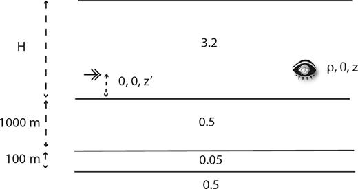
The canonical reservoir model used throughout this paper. The source (double arrow) is located at (0, 0, z΄) and the observation point (eye) is at (ρ, 0, z), where the middle coordinate is the azimuth φ. The ocean layer of thickness H and conductivity 3.2 S m−1 is overlain by an insulating atmosphere and underlain by a two layer structure in turn underlain by a half-space. The overburden and underburden have a conductivity of 0.5 S m−1 (resistivity of 2 Ω m) and the reservoir layer between 1000 and 1100 m depth has a conductivity of 0.05 S m−1 (resistivity of 20 Ω m).
The ratio of the displacement to the conduction current in CSEM may be represented by the dimensionless number εω/σ, where ε is the electric permittivity, ω is the source angular frequency and σ is the electrical conductivity. Using the canonical model, it is easy to show that displacement current is no more than 10−8 times the conduction current in the reservoir layer at an upper frequency limit of 10 Hz, and is even smaller elsewhere in the structure or at lower frequencies. Further, it is not necessary to consider displacement current in the insulating air above the ocean provided that the source–receiver offset is small compared to the free-space wavelength (Nekut & Spies 1989; Chave 2009), which as a matter of practice always holds.
Thus, the pre-Maxwell equations without displacement current are sufficient throughout the structure, and the physics is that of diffusion driven by a continuous, temporally periodic source. The consequence is an EM field that evolves unidirectionally forward in time at all points away from a source because the operation t → −t does not leave the governing equations invariant. Diffusion cannot run backward in time, unlike wave propagation. Further, Morse & Ingard (1968, p. 479) show that any physical system whose phase velocity approaches infinity as frequency goes to infinity cannot exhibit wave fronts. The phase velocity for marine CSEM is proportional to |$\sqrt \omega $|, hence its physics does not incorporate wave fronts. The absence of wave fronts precludes the existence of Huygens-type reflection (and concomitantly, refraction) at interfaces (see also Mandelis et al. 2001).
Further, diffusive systems like CSEM respond to a driving source simultaneously at all points within it, and so the EM response at a given point in a conductive medium is influenced by the resistivity of the entire structure. Simultaneity in diffusion physics can be understood at a microscopic level through seminal work by Einstein (1905), who established a direct relationship between macroscopic and microscopic diffusion. Diffusion is a consequence of the random, thermally driven motion of an ensemble of microscopic particles whose drift velocity is described by a probability distribution, and hence diffusion involves stochasticity. As a consequence, particles whose velocity is given by the distribution tails will drift very quickly, so that the particles comprising a diffusive system rapidly evolve to a steady state on a global basis. For marine CSEM, the microscopic particles are the charge carriers throughout the resistivity structure that are subject to drift when a source current is applied. They reach steady state on a timescale that is very short compared to the CSEM timescale of one over the source frequency.
Chave (2009) presented Green's functions for the fundamental and independent poloidal and toroidal magnetic (PM and TM) modes that describe CSEM fields in a 1-D structure produced by a point HED, including all of the interactions between the air–water interface and the subsurface resistivity structure, and obtained the field components for an HED source within the ocean layer. It is well known that the enhanced EM response at a given offset to a resistive reservoir model compared to that of a half-space with the reservoir model overburden resistivity is a galvanic TM mode phenomenon, while the air interaction is an inductive PM mode response. Fig. 11 in Chave (2009) shows this graphically by comparing the intermediate water depth Poynting vectors for vertical magnetic and electric dipoles that solely produce PM and TM modes, respectively.
The EM fields within the layered structure may easily be derived by matching solutions to the homogeneous forms of the modal equations at the seafloor to the Green's functions using appropriate boundary conditions, and may be propagated down to the depth of interest. Such solutions will be used to estimate the Poynting vector and Joule heating throughout the conductive structure.
For continuous, time harmonic forcing, Chave (2009) also showed that the time average (over a complete cycle of the source) of S is equal to the real part of the complex Poynting vector |${\boldsymbol S} = ( {{{\bf E}} \times {{{\bf B}}^*}} )/( {2{\mu _{\rm{o}}}} )$| (where the superscript * denotes the complex conjugate; note that |${{\bf S}} \ne {\boldsymbol S}$|) that represents the time-averaged energy flux into a volume of material that is balanced by Joule heating within it; Stratton (1941, section 2.20) gives a similar derivation. The real part of the complex Poynting vector was used by Chave et al. (1990) to visualize the time-averaged energy flux for an earth model containing a low conductivity lithospheric zone bounded above and below by higher conductivity regions. Weidelt (2007) and Chave (2009) presented analogous results for a hydrocarbon reservoir model.
The EM fields produced in CSEM have a 3-D vector rather than a scalar form, and hence the standard practice of evaluating the amplitude and/or phase of a single Cartesian field component against offset or frequency is not sufficient for understanding their behaviour. It is well known that a time harmonic vector field can be depicted as a polarization ellipse oriented appropriately in space, and this representation serves as a complete description of the field. Further, when an ellipse is required to depict the EM field, its Cartesian components are not independent.
Chave (2009) derived a representation for elliptically polarized EM fields that utilizes six parameters: the amplitude of the semi-major axis a, the ratio of the semi-minor to the semi-major axis amplitudes or ellipticity, the generalized phase ϕ, the strike θ of the semi-major axis in the ellipse plane, the roll ξ around the semi-major axis and the pitch ψ around the semi-minor axis. All of the angles are positive counter-clockwise. There is an inherent ambiguity in this representation, as it is unchanged if any pair of (θ, ϕ), (θ, ξ) and (ξ, ϕ) are altered by 180°. For the in-line geometry of this paper, the polarization ellipse is degenerate such that the pitch ψ is always zero and the roll ξ is ±90°, so the ellipse is oriented in the x–z plane with the tip of the electric field vector rotating counter-clockwise or clockwise as the roll is negative or positive. The roll will be set to −90°, so that only the strike and ellipticity are need to characterize the degenerate polarization ellipse for the in-line orientation. Fig. 2 depicts this case. The generalized phase will be assumed continuous, so the representation ambiguity can easily be resolved. Note also that the sense of ellipse rotation has nothing to do with the temporal variation of the EM field; the tip of the electric field vector moves around the ellipse at the driving frequency of the source, while the ellipse orientation and the sense of rotation can change with source–receiver offset or frequency.
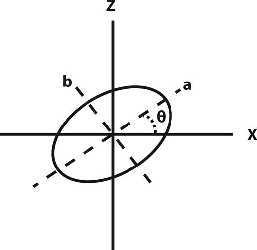
Electric field polarization ellipse for the degenerate in-line case of this paper. The semi-major axis a and the semi-minor axis b are shown by dashed lines. The strike θ is the angle between the x-axis and the semi-major axis.
3 MODEL RESULTS
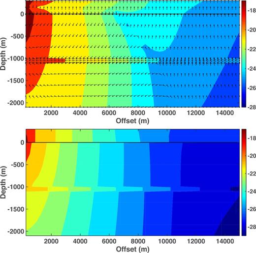
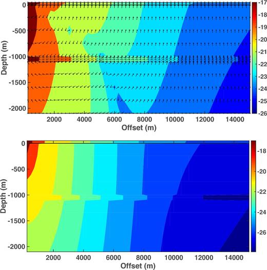
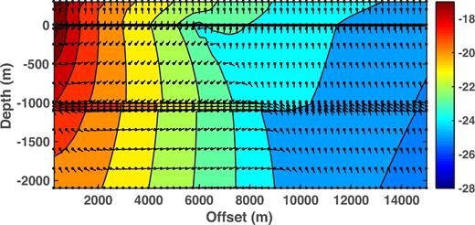
Fig. 3 shows the real part of the complex Poynting vector (hereafter simply Poynting vector) and Joule heating as a function of offset and depth for a source frequency of 0.1 Hz and a water layer thickness of 2000 m. The source is a point dipole with unit moment throughout this paper. At this frequency, the skin depth in seawater (overburden) is 890 m (2.3 km), so the source is about 2.2 skin depths below the sea surface and about 0.4 skin depth above the reservoir, and hence the excitation of the reservoir should dominate the air interaction except possibly at large source–receiver offsets. The Poynting vector and Joule heating plots show the base 10 logarithm of the magnitude of each quantity in colour scale; note that the units of the Poynting vector are watts per m2 while the dissipation term is in watts per m3, and so the colour scales are not equivalent. The Poynting vector plot also shows the direction of energy flow at each of the small circles throughout the structure. Fig. 3 is similar to the deep (5000 m) water result of Chave (2009; bottom panel of fig. 16), and is dominated by nearly horizontal energy flow away from the source within the reservoir layer that leaks into the overburden, decreasing monotonically with offset. The dominantly horizontal Poynting vector is due to a largely vertical electric field in the reservoir layer. For a given offset, both the Poynting vector and Joule heating magnitude are largest within the reservoir layer, and the tongues of energy flux or dissipation extend further outward as offset increases to ∼8 km, then become substantially the same length. The energy flux within the water layer is primarily upward away from the seafloor, although a weak air interaction is apparent at the longest offsets, and is manifest as downward energy flux within the water layer that extends nearly to the seafloor at 15 km. There is a narrow transition zone within the water layer that separates dominance by the direct effects of the dipole source (including reservoir energy flow) from dominance by the air interaction. If the reservoir layer were absent, an analogous transition zone would appear at a shorter offset due to the lack of guided energy flow in the substrate.
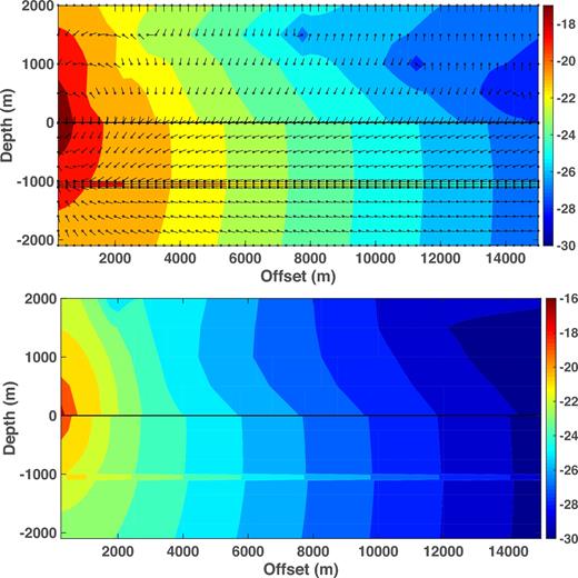
Contours of the logarithms (base 10) of the magnitudes of the Poynting vector (top) and Joule heating (bottom) as a function of source–receiver offset and depth for the model of Fig. 1. The water depth is 2000 m, the source frequency is 0.1 Hz and the point source lies 30 m above the seafloor at the origin. The seafloor is depicted by a solid horizontal black line. The Poynting vector plot also shows the direction of energy flow at each of the small circles throughout the structure. The arrow orientations have been adjusted for the different horizontal and vertical scales.
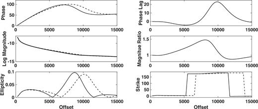
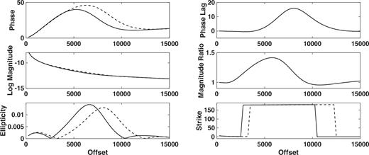
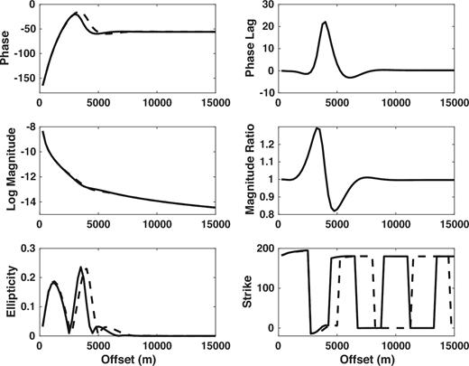
The seafloor electric field (Fig. 4) is depicted as the generalized phase lag of the reservoir model relative to the half-space one and the ratio of the electric field amplitude for the reservoir model of Fig. 1 to that of a half-space of resistivity 2 Ω m (upper and middle right panels), in both cases against source–receiver offset. The remaining panels show the ellipse amplitude/phase and orientation parameters for both the reservoir and half-space models as described in Section 2. As a function of offset, the amplitude ratio (phase lag) is monotonically increasing (decreasing, except at the largest values), exhibiting a change in slope at ∼2.5 km (or about 3 skin depths in seawater) as the electric field flowing directly from the source in the water layer attenuates away, and a second change in slope at large offsets as the effect of the downward energy flux in the water layer in Fig. 3 reaches the seafloor. This appears in the phase lag at a shorter offset than in the amplitude. An amplitude ratio greater than unity and a negative phase lag indicate that the response of the reservoir model is stronger and faster compared to that of a half-space.
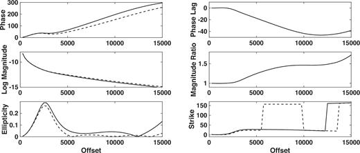
The polarization ellipse representation of the seafloor electric field as a function of offset from an HED point source placed at the origin but 30 m above the seafloor. The water depth is 2000 m and the source frequency is 0.1 Hz. From the upper left and proceeding counter-clockwise, the panels show the phase of the reservoir and half-space responses, the base 10 logarithm of the magnitude of the reservoir and half-space responses, the ellipticity, the strike θ of the semi-major axis in the ellipse plane, magnitude ratio of the reservoir to the half-space response and the phase lag between the reservoir and half-space responses. For the first four panels, the dashed line is the reservoir result while the solid line is the half-space result.
There is complex orientation behaviour that occurs along with the changes in amplitude and phase. For the reservoir model at offsets to ∼5.5 km, the ellipticity is as large as 0.3 and the semi-major axis yaws slowly counter-clockwise in the x–z plane. From ∼5.5 to ∼10 km, the semi-major axis yaws counter-clockwise through ∼140° and becomes nearly linearly polarized. The ellipse then shifts sharply clockwise out to ∼14 km, when it flips again. The half-space model does not display a shift in orientation until an offset of ∼13 km and has a slightly higher ellipticity than the reservoir model.
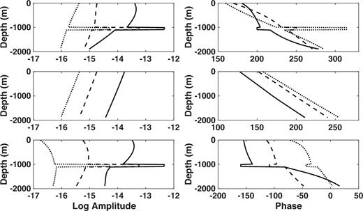
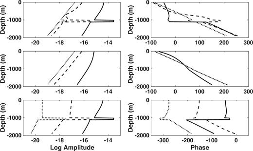
Fig. 5 shows the in-line electric field Fréchet derivatives with respect to conductivity, and their PM and TM mode components, at source–receiver offsets of 3, 7 and 11 km for the model of Figs 2 and 3. The TM mode is preferentially sensitive to conductivity changes within the resistive reservoir layer, while the PM mode is insensitive to the reservoir conductivity. This is an expected consequence of the heightened galvanic response, relative to the modest inductive response, to a buried resistive layer. The TM mode amplitude is substantially (by 1–2 orders of magnitude) larger than the PM mode amplitude in the overburden and reservoir layer at large offsets, but the PM mode is influential within the over and underburden at short to intermediate offsets. There is also a large change in phase across the reservoir layer for the TM mode at short offset that is also present for the total Fréchet derivative. The total Fréchet derivative is smaller than either the PM or TM mode components in the underburden because the modes are nearly out of phase in that region.
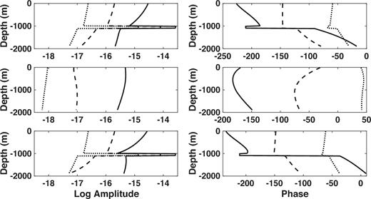
The Fréchet derivatives of the in-line seafloor electric field as a function of depth below the seafloor for a point HED source located at the origin but 30 m above the seafloor. The water depth is 2000 m and the source frequency is 0.1 Hz. The left-hand panels show the logarithm of the magnitude and the right-hand panels show the phase. From top to bottom, the rows show the total Fréchet derivative, the PM mode component and the TM mode component. The different curves correspond to offsets of 3 km (black), 7 km (dashed) and 11 km (dotted).
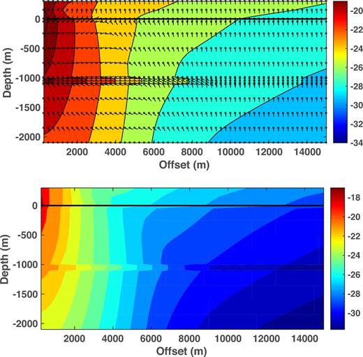
Fig. 6 shows the Poynting vector and Joule heating for an intermediate water depth of 300 m and a 0.1 Hz source; the electrical thickness is about 0.3 skin depth in the water layer and 0.4 skin depth in the overburden, so the air interaction is expected to play a stronger role than for 2000 m water depth. The effect of the air interaction is quite evident compared to Fig. 3, and is seen as an abrupt shift from upward to downward energy flow at the seafloor at ∼6.5 km offset, and the propagation of this reversal downward to the reservoir layer at ∼9.5 km offset. At this point, the direction of energy flux in the reservoir layer shifts from outward horizontal to nearly vertical downward, but with an inward component, then becomes vertical and finally has an outward component at the longest offsets. These transitions reflect increasing dominance by the inductive air interaction as the offset rises, resulting in replacement of galvanically driven guided energy flow in the reservoir layer with an inductively driven vertical energy flux.
Contours of the logarithms (base 10) of the magnitudes of the Poynting vector (top) and Joule heating (bottom) as a function of source–receiver offset and depth for the model of Fig. 1. The water depth is 300 m, the source frequency is 0.1 Hz and the point source lies 30 m above the seafloor at the origin. The seafloor is depicted by a solid horizontal black line. The Poynting vector plot also shows the direction of energy flow at each of the small circles throughout the structure. The arrow orientations have been adjusted for the different horizontal and vertical scales.
The Poynting vector in the overburden mirrors this behaviour, while in the underburden the energy flux has an upward component beyond ∼4 km that shifts downward beyond ∼10 km. The underburden energy flux is distinct from that in deeper water (Fig. 3). The Joule heating is similar to that for deep water (Fig. 3) except that the largest values at a given offset occur in both the water and reservoir layers, and the reservoir tongue does not extend further outward as offset increases.
The seafloor electric field for the intermediate water depth model (Fig. 7) initially shows a positive amplitude ratio over ∼2.5–10 km and a weak phase lead over ∼2.5–7 km, followed by a decrease in amplitude ratio that becomes slightly smaller than unity out to the longest offset, and a phase that lags the half-space value out to ∼14 km, peaking at ∼9 km. Consequently, the reservoir response is initially stronger and faster (∼0–7 km) than the half-space response, then becomes stronger and slower (∼7–10 km), and finally transitions to weaker and slower at large offsets. The phase lag changes sign at a shorter offset than the amplitude ratio. This behaviour is accompanied by concomitant changes in the ellipse shape. At offsets below ∼6 km for the reservoir model, the polarization is nearly linear and the semi-major axis is yawed slightly clockwise. Beyond this offset, the polarization is more elliptical and the semi-major axis shifts sharply counter-clockwise through ∼180° and then shifts clockwise through the same angle at 14 km offset. The half-space model displays similar behaviour but at shorter offsets, reflecting that field enhancement due to the reservoir layer is absent.
The polarization ellipse representation of the seafloor electric field as a function of offset from an HED point source placed at the origin but 30 m above the seafloor. The water depth is 300 m and the source frequency is 0.1 Hz. From the upper left and proceeding counter-clockwise, the panels show the phase of the reservoir and half-space responses, the base 10 logarithm of the magnitude of the reservoir and half-space responses, the ellipticity, the strike θ of the semi-major axis in the ellipse plane, magnitude ratio of the reservoir to the half-space response and the phase lag between the reservoir and half-space responses. For the first four parameters, the dashed line is the reservoir result while the solid line is the half-space result.
Fig. 8 shows the in-line electric field Fréchet total derivative, and its PM and TM mode components, for the intermediate water depth model. As in Fig. 5, the TM mode is dominant within the reservoir layer at all offsets shown, and in fact the TM mode curves are quite similar in Figs 5 and 8. However, the PM mode component has a discernible effect within the overburden and underburden at all offsets, as evidenced by comparing the amplitude of the PM and TM modes.
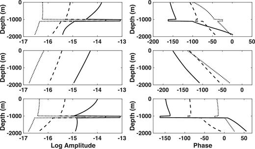
The Fréchet derivatives of the in-line seafloor electric field as a function of depth below the seafloor for a point HED source located at the origin but 30 m above the seafloor. The water depth is 300 m and the source frequency is 0.1 Hz. The left-hand panels show the logarithm of the magnitude and the right-hand panels show the phase. From top to bottom, the rows show the total Fréchet derivative, the PM mode component and the TM mode component. The different curves correspond to offsets of 3 km (black), 7 km (dashed) and 11 km (dotted).
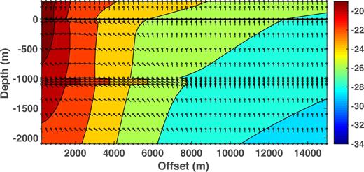
Fig. 9 shows the Poynting vector and Joule heating for shallow (50 m) water and a 0.1 Hz source. The water layer has an electrical thickness of about 0.06 skin depth compared to 0.4 skin depth in the overburden, and hence the air interaction can be expected to be important at most offsets. The Poynting vector plot is qualitatively similar to that in Fig. 6, except that changes in direction occur at smaller offsets throughout the structure and the direction of energy flux in the reservoir layer is fully reversed at offsets beyond ∼5 km, gradually rotating downward and then slightly outward at longer distances. As a consequence of the energy flux confluence at ∼5 km in the reservoir layer, the flow direction in the underburden abruptly shifts from upward, outward to downward, inward. A minimum in the Poynting vector amplitude is also observed extending from near the source downward to the reservoir layer at ∼5 km and then further into the underburden. The locus of the minimum represents a shift from dominance by the dipole source (including galvanic reservoir excitation) to dominance by the air interaction. The outward energy flux tongue in the reservoir layer decreases in length up to ∼5 km, then increases over the interval exhibiting reversed energy flux and ultimately gets smaller at the longest source–receiver offsets. Joule heating is largest in the water layer at a given offset beyond ∼5 km. Dissipation in the overburden is larger than that in the reservoir layer at a given offset beyond ∼8 km, and the reservoir layer becomes a locus of minimum dissipation at the longest offsets.
Contours of the logarithms (base 10) of the magnitudes of the Poynting vector (top) and Joule heating (bottom) as a function of source–receiver offset and depth for the model of Fig. 1. The water depth is 50 m, the source frequency is 0.1 Hz and the point source lies 30 m above the seafloor at the origin. The seafloor is depicted by a solid horizontal black line. The Poynting vector plot also shows the direction of energy flow at each of the small circles throughout the structure. The arrow orientations have been adjusted for the different horizontal and vertical scales.
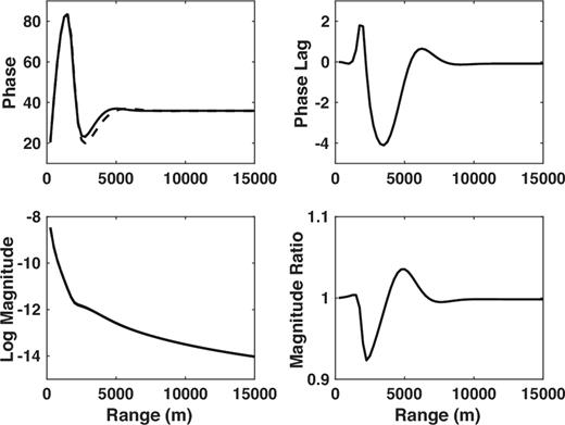
Fig. 10 shows the seafloor electric field for the shallow water model of Fig. 9. The amplitude ratio is greater than unity over ∼2–9 km, and becomes very weakly negative beyond that point out to ∼12 km. The phase for the reservoir model lags that for a half-space over ∼5–12 km, and has a weak lead at shorter offsets. Consequently, the reservoir response is stronger and slightly faster at short (∼0–5 km) offsets, substantially stronger and slower at intermediate (∼5–9 km) offsets, then becomes weaker and slower at large offsets. The polarization is nearly linear at all offsets. The strike of the semi-major axis shifts counter-clockwise through ∼180° at about 3 km offset and then clockwise back at ∼12.5 km. Overall, the seafloor electric field is an attenuated version of the intermediate water depth result in Fig. 7, with the additional influence of the flux reversal in the reservoir layer.
The polarization ellipse representation of the seafloor electric field as a function of offset from an HED point source placed at the origin but 30 m above the seafloor. The water depth is 50 m and the source frequency is 0.1 Hz. From the upper left and proceeding counter-clockwise, the panels show the phase of the reservoir and half-space responses, the base 10 logarithm of the magnitude of the reservoir and half-space responses, the ellipticity, the strike θ of the semi-major axis in the ellipse plane, the magnitude ratio of the reservoir to the half-space response and the phase lag between the reservoir and half-space responses. For the first four parameters, the dashed line is the reservoir result while the solid line is the half-space result.
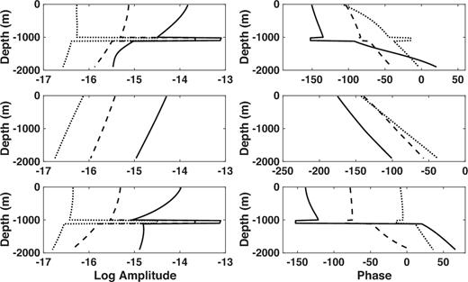
Fig. 11 shows the Fréchet derivatives of the in-line electric field, and its PM and TM mode components, for the shallow water model of Figs 9 and 10. The phase sensitivity to the reservoir is not as large as in Fig. 8. In addition, the effect of the PM mode is enhanced over that for the intermediate depth model, and it plays a major role throughout the overburden and underburden at all offsets.
The Fréchet derivatives of the in-line seafloor electric field as a function of depth below the seafloor for a point HED source located at the origin but 30 m above the seafloor. The water depth is 50 m and the source frequency is 0.1 Hz. The left-hand panels show the logarithm of the magnitude and the right-hand panels show the phase. From top to bottom, the rows show the total Fréchet derivative, the PM mode component and the TM mode component. The different curves correspond to offsets of 3 km (black), 7 km (dashed) and 11 km (dotted).
Fig. 12 shows the Poynting vector and Joule heating for the 300 m water layer of Fig. 6 but with a 1 Hz source. At this frequency, the skin depth in seawater is 280 m, and hence comparable to the water depth, while the overburden is about 1.4 skin depths thick, and hence the reservoir effect should be dwarfed by the influence of the sea surface beyond some offset. By comparison with Fig. 6, the magnitudes of the Poynting vector and Joule heating are smaller at a given offset and depth, reflecting greater attenuation throughout the structure due to the higher frequency. The seafloor energy flux shifts from upward to downward at a source–receiver offset of ∼3.5 km, and the flip in direction propagates downward to the reservoir layer at ∼5.5 km. The time-averaged energy flux is downward throughout the structure beyond ∼9.5 km, and the rightward tongue of enhanced energy flux vanishes. This reflects the fact that, at the relatively high frequency of 1 Hz, the dipole field is heavily attenuated at long range, whereas the spatially broad field due to the air interaction is not. Concomitantly, dissipation is largest within the reservoir layer only at small offsets, becoming comparable within the overburden beyond ∼5.5 km and then turning to a local minimum of dissipation.
Contours of the logarithms (base 10) of the magnitudes of the Poynting vector (top) and Joule heating (bottom) as a function of source–receiver offset and depth for the model of Fig. 1. The water depth is 300 m, the source frequency is 1 Hz and the point source lies 30 m above the seafloor at the origin. The seafloor is depicted by a solid horizontal black line. The Poynting vector plot also shows the direction of energy flow at each of the small circles throughout the structure. The arrow orientations have been adjusted for the different horizontal and vertical scales.
Fig. 13 shows the seafloor electric field corresponding to Fig. 12, and resembles a compressed and attenuated version of Fig. 7. The amplitude for the reservoir model is initially larger than that for a half-space, peaking at ∼3 km, and then decreases to a value smaller than for a half-space before becoming the same beyond ∼8 km. The phase lags that for a half-space only over ∼3–5 km, leads slightly on either side of those values and is nearly the same as that for a half-space beyond ∼9 km. Consequently, the reservoir model response is initially slightly stronger and faster (∼2–3 km), then stronger and slower (∼3–4 km), and finally weaker and slower (∼4–7 km), as compared to the half-space response. The ellipticity has dual peaks at about 1 and 4 km, and is larger than at 0.1 Hz in Fig. 7. The strike changes repeatedly with offset, but is similar over 0–8 km to the entire range of Fig. 7.
The polarization ellipse representation of the seafloor electric field as a function of offset from an HED point source placed at the origin but 30 m above the seafloor. The water depth is 300 m and the source frequency is 1 Hz. From the upper left and proceeding counter-clockwise, the panels show the phase of the reservoir and half-space responses, the base 10 logarithm of the magnitude of the reservoir and half-space responses, the ellipticity, the strike θ of the semi-major axis in the ellipse plane, magnitude ratio of the reservoir to the half-space response and the phase lag between the reservoir and half-space responses. For the first four parameters, the dashed line is the reservoir result while the solid line is the half-space result.
The PM mode Frèchet derivatives (Fig. 14) show the strong influence of the air interaction beyond 3 km offset, and dominates the TM mode component in the overburden and underburden beyond 7 km offset. There is very little enhanced sensitivity to the reservoir layer at 11 km offset. The PM mode phase is nearly identical at 7 and 11 km offset, reflecting dominance by the air interaction.
The Fréchet derivatives of the in-line seafloor electric field as a function of depth below the seafloor for a point HED source located at the origin but 30 m above the seafloor. The water depth is 300 m and the source frequency is 1 Hz. The left-hand panels show the logarithm of the magnitude and the right-hand panels show the phase. From top to bottom, the rows show the total Fréchet derivative, the PM mode component and the TM mode component. The different curves correspond to offsets of 3 km (black), 7 km (dashed) and 11 km (dotted).
Fig. 15 shows the Poynting vector for 300 m water depth and a 0.1 Hz source in the shallow towed configuration, with the source at 10 m below the sea surface and the receivers at 100 m below the sea surface. It is very similar to the seafloor configuration result in Fig. 6, with the key feature of transition from upward, outward to downward, inward energy flux at the seafloor and its propagation through the overburden, occurring at about a 1 km shorter offset. The Joule heating for the shallow towed model is nearly identical to that in Fig. 6, and is omitted.
Contours of the logarithm (base 10) of the magnitude of the Poynting vector as a function of source–receiver offset and depth for the model of Fig. 1. The water depth is 300 m, the source frequency is 0.1 Hz and the point source lies 10 m below the sea surface at the origin. The receivers lie at 100 m water depth in the shallow towed configuration. The seafloor is depicted by a solid horizontal black line. The Poynting vector plot also shows the direction of energy flow at each of the small circles throughout the structure. The arrow orientations have been adjusted for the different horizontal and vertical scales.
It is not practical to measure the vertical electric field from a towed streamer, hence Fig. 16 shows the in-line electric field parameters corresponding approximately to the four upper panels in Fig. 7. The shallow towed electric field is very similar to the seafloor one for this model, displaying an initial stronger and very slightly faster reservoir response from ∼2 to 6 km offset, then a stronger and slower response to ∼9 km, a weaker and slower response to ∼12.5 km, and finally a slight weaker and faster response to the largest offsets. The transitions for the shallow towed configuration in Fig. 16 systematically occur at 1–2 km shorter offsets as compared to the seafloor configuration model in Fig. 7.
The in-line electric field at 100 m water depth as a function of offset from an HED point source placed at the origin but 10 m below the sea surface. The water depth is 300 m and the source frequency is 0.1 Hz. From the upper left and proceeding counter-clockwise, the panels show the phase of the reservoir and half-space responses, the base 10 logarithm of the magnitude of the reservoir and half-space responses, the magnitude ratio of the reservoir to the half-space response and the phase lag between the reservoir and half-space responses. The dashed line is the reservoir result while the solid line is the half-space result.
Fig. 17 shows the Fréchet derivatives for the shallow towed configuration model in Fig. 15. It is only subtly distinct from Fig. 8, with the largest difference occurring for the PM mode, which is slightly stronger and displays a higher phase compared to the seafloor configuration. This reflects a stronger air interaction for the towed configuration due to proximity to the sea surface. The TM mode result is nearly identical to that in Fig. 8.
The Fréchet derivatives of the in-line 100 m water depth electric field as a function of distance below the seafloor for a point HED source located at the origin but 10 m below the sea surface. The water depth is 300 m and the source frequency is 0.1 Hz. The left-hand panels show the logarithm of the magnitude and the right-hand panels show the phase. From top to bottom, the rows show the total Fréchet derivative, the PM mode component and the TM mode component. The different curves correspond to offsets of 3 km (black), 7 km (dashed) and 11 km (dotted).
Fig. 18 contains the Poynting vector for 300 m water depth and a 1 Hz source in the shallow towed configuration. The receivers are located 100 m below the sea surface, hence about 3/4 skin depth from the seafloor, so that the electric field produced by the subsurface will be attenuated by about 1/3 compared to the seafloor configuration in Fig. 12, and the effect of the sea surface will be increased. This is manifest as key features in Fig. 18 occurring at 1–2 km smaller offsets compared to Fig. 12; for example, the transition from upward to downward energy flux at the seafloor occurs at 1.5 km in Fig. 18, but 3 km in Fig. 12. The Joule heating corresponding to Fig. 18 is very similar to that in Fig. 12, and is omitted.
Contours of the logarithms (base 10) of the magnitudes of the Poynting vector as a function of source–receiver offset and depth for the model of Fig. 1. The water depth is 300 m, the source frequency is 1 Hz and the point source lies 10 m below the sea surface at the origin. The receivers are at 100 m water depth. The seafloor is depicted by a solid horizontal black line. The Poynting vector plot also shows the direction of energy flow at each of the small circles throughout the structure. The arrow orientations have been adjusted for the different horizontal and vertical scales.
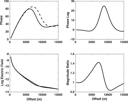
Fig. 19 shows the electric field at 100 m water depth for the towed configuration, which resembles an attenuated Fig. 13 that is compressed toward the origin. There are additional differences due the absence of the vertical electric field in Fig. 19. Overall, the anomaly signal for the towed configuration is much smaller than for the seafloor configuration, with a phase lag range of 6° compared to about 30°.
The in-line electric field at 100 m water depth as a function of offset from an HED point source placed at the origin but 10 m below the sea surface. The water depth is 300 m and the source frequency is 1 Hz. From the upper left and proceeding counter-clockwise, the panels show the phase of the reservoir and half-space responses, the base 10 logarithm of the magnitude of the reservoir and half-space responses, the magnitude ratio of the reservoir to the half-space response and the phase lag between the reservoir and half-space responses. The dashed line is the reservoir result while the solid line is the half-space result.
Fig. 20 shows the Frèchet derivatives for 300 m water depth for the model of Fig. 18. The result differs only slightly from the seafloor configuration counterpart in Fig. 14, with the TM mode in the under and overburden attenuated by a factor of 2–3, but nearly unchanged in the reservoir layer. By contrast, the PM mode for the two receiver locations is nearly identical, and the result is slightly lower sensitivity outside the reservoir layer in the total Frèchet derivative.

The Fréchet derivatives of the in-line 100 m water depth electric field as a function of distance below the seafloor for a point HED source located at the origin but 10 m below the sea surface. The water depth is 300 m and the source frequency is 1 Hz. The left-hand panels show the logarithm of the magnitude and the right-hand panels show the phase. From top to bottom, the rows show the total Fréchet derivative, the PM mode component and the TM mode component. The different curves correspond to offsets of 3 km (black), 7 km (dashed) and 11 km (dotted).
4 DISCUSSION
The Poynting vector results in Figs 3, 6, 9, 12, 15 and 18 reflect the competing effects of the dipole source (including galvanic, guided energy flow within the reservoir) and the inductive air interaction, along with coupling of the two EM modes. For the seafloor configuration, when the ocean is more electrically thick than the overburden (Fig. 3), the air interaction does not appear except at the longest offsets within the ocean, and is never seen below it out to 15 km offset. When the electrical thicknesses of the water layer and overburden are comparable (Figs 6 and 12), the dipole source and guided energy flow are predominant at short offsets, and the air interaction is larger at long offsets, yielding a sharp transition zone that moves from the water layer through the overburden and into the underburden. This is manifest in Figs 6 and 12 as the increasingly upward tilt of the energy flux in the underburden beyond 5 km that shifts downward beyond ∼10 km, and clearly demonstrates that the air interaction couples into the entire structure rather than being due simply to the direct influence of the sea surface. For comparison, Fig. 3 for 2000 m water depth has subhorizontal outward energy flow in the underburden at all offsets. For an ocean that is electrically quite thin compared to the overburden (Fig. 9), the transition zone begins at nearly zero offset in the water layer, and the cross-mode terms in (3) are polarized appropriately, and strong enough, at the reservoir layer to reverse the time-averaged energy flux direction over 5–9 km offset. This phenomenon cannot be solely due to either the PM or TM modes, as witnessed by fig. 11 in Chave (2009). A similar flux reversal is observed for the shallow towed configuration at the same water depth and frequency.
For the shallow towed configuration, there is additional attenuation of both the source and received signals because the source and receivers are located near the sea surface. For 300 m water depth and 0.1 Hz, this produces only small differences between the seafloor and shallow towed configuration models, but somewhat larger differences at 1 Hz.
These observations do depend on the resistivity contrast between the reservoir layer and the overburden. The results in this paper pertain to a 10:1 resistivity contrast. Lower contrasts are frequently observed, and can even be reversed in shaly sands or carbonate host formations (Worthington 2000), while contrasts of 100:1 are quite rare. In the presence of a higher resistivity contrast, the effect of the galvanic reservoir will be stronger for a given offset and water depth, and hence the transitions noted regarding the Poynting vector, Joule heating and electric field will move to longer offsets. Conversely, if the resistivity contrast is weaker or there is no reservoir, the air interaction will become important at shorter offsets, and the transitions will move in that direction.
The Joule heating can easily be understood in terms of continuity of vertical electric current versus continuity of the in-line electric field at the reservoir layer boundaries. For deep water (Fig. 3), the electric field is nearly vertical within the reservoir layer at all ranges. Consequently, by continuity of vertical electric current, the vertical electric field in the reservoir must be an order of magnitude larger than in the overburden or underburden because the reservoir conductivity is 1/10 that in those regions, implying that Joule heating is always enhanced within the reservoir layer at a given offset. However, as the air interaction predominates over the galvanic reservoir response (Figs 6, 9, 12, 15 and 18), the electric field becomes increasingly radial, and hence will have the same value in the reservoir layer and overburden/underburden, resulting in reduced Joule heating because the reservoir conductivity is lower than in its surroundings.
When expressed as the ratio of the magnitude of the reservoir response to that of a half-space with the overburden resistivity, and the phase lag between the reservoir and the half-space model, both as a function of source–receiver offset, the amplitude ratio consistently peaks where the phase lag is changing most rapidly. Consequently, a phase response to a structure is always observed at shorter ranges than an amplitude response. This is clearly observed in the electric field for Figs 4, 7, 10, 13, 16 and 19.
The behaviours of the seafloor electric and magnetic fields are tightly associated with energy flow through the entire conductive structure, with regions where the Poynting vector magnitude is large having a stronger relation, and points that are distant having a weaker relation than those nearby. Fig. 3 shows no effect of the downward propagating energy in the water layer at or beneath the seafloor, but only above it. However, the seafloor electric field in Fig. 4 clearly reflects its presence beyond ∼12 km offset. At all offsets, guided energy flow in the reservoir layer is associated with a consistently stronger and faster response compared to a half-space.
When the electrical thicknesses of the water layer and overburden are comparable, Figs 7 and 13 show that the amplitude of the reservoir model is initially larger than that for a half-space, then is weaker at longer offsets, while the reservoir phase initially leads that of a half-space, and then lags it. The enhanced amplitude is associated with guided energy flow in the reservoir layer, and the transition to a weaker response occurs when the horizontal energy flux in it is impacted by the air interaction (Figs 6 and 12). The initial phase lead for the reservoir model reflects the dominating influence of guided energy flow in the reservoir layer that is increasingly counteracted by downward energy flux from the air interaction; the direction of energy flow at the seafloor shifts from upward to downward approximately at the inflection point in the phase. Conversely, the phase lag for the reservoir model at longer ranges is due to the increasing importance of the air interaction relative to guided energy flow, particularly in the overburden.
When the ocean is electrically much thinner than the overburden, Fig. 10 shows that a reservoir response with a greater magnitude than that of a half-space precedes a weaker one at longer ranges, although the corresponding source–receiver offsets are smaller than for an intermediate water depth. However, the phase for the reservoir layer lags that of a half-space model in Fig. 10, and never really leads it. The enhanced amplitude in Fig. 10 occurs at source–receiver offsets where energy flow (Fig. 9) in the reservoir layer is nearly horizontal (although it reverses direction at ∼5 km) and the Poynting vector magnitude is comparable to or larger than that near the seafloor. The peak phase lag occurs where the energy flux becomes dominantly inward in the reservoir layer and downward in the overburden.
Comparison of Figs 7 & 16, and 13 & 19, shows that the transitions observed in the seafloor configuration occur at shorter offsets for the shallow towed configuration. Further, they are substantially smaller for both amplitude and phase in the towed configuration, consistent with attenuation in the conductive water layer. However, they display the same characteristic for the seafloor configuration of a peak in phase lag occurring where the magnitude is changing most rapidly.
The ellipse parameters in Figs 4, 7, 10 and 13 are complicated, and are not substantially simpler for a half-space as compared to a reservoir model. The 180° change in strike for the reservoir model at ∼6 km in Fig. 7 occurs near the point in Fig. 6 where the seafloor energy flux flips from upward, weakly outward to downward, weakly inward. Concomitantly, the ellipticity increases beyond that point. A similar effect is seen in Figs 12 and 13 at a range of ∼3 km. However, this is obscured in Figs 9 and 10 by reversal of the energy flux direction in the reservoir layer over ∼5–9 km.
The results of this paper explore the complexity of the physics of marine CSEM in shallow water for an isotropic model. The physics is governed by two competing phenomena: the direct effect of a dipole source, including guided energy flow within a resistive zone representative of an oil reservoir, and an air interaction that manifests as the intricate flow of energy throughout the resistivity structure caused by an electrically thin water layer. The way these two processes compete to produce the measurement variables (i.e. the EM fields at the seafloor) depends on the entire electrical structure in a complex manner. Certainly, characterization of the air interaction as an ‘up-over-down’ mode that occurs entirely within the water layer is wholly inadequate. It is hoped that the results of this paper combined with those of Andréis & MacGregor (2008) will finally put that oversimplification to rest.
The results of this paper also show that CSEM in intermediate to shallow water remains sensitive to subsurface resistive structures, an observation that has previously been made by Mittet (2008) on the basis of a larger magnitude response for shallow over deep water. This is most easily seen through the Fréchet derivatives in Figs 5, 8, 11, 14, 17 and 20, and is due to the substantial sensitivity of the TM mode to low conductivity media that is not overcome by the PM mode air interaction except in very shallow water at higher frequencies.
Finally, it is widely believed (e.g. MacGregor & Sinha 2000) that an HED source in the in-line and broadside geometries produces principally vertical and horizontal electric currents, respectively. It has also long been known that continental shelf sedimentary formations display a transversely anisotropic electrical conductivity (by a factor of 2–3, and up to 10), with the vertical component of conductivity being smaller than the horizontal one. This has been recognized to be an important issue for marine CSEM (e.g. Tompkins et al. 2004; Ramananjaona et al. 2011; Mattsson et al. 2013), and consequently seafloor measurements over a wide range of source–receiver geometries would be needed to resolve both the anisotropy and the reservoir structure, with the in-line orientation primarily sensitive to the vertical conductivity and the broadside one sensitive to the horizontal conductivity. This would appear to militate against using the strictly in-line geometry discussed in this paper. However, it is very clear from the Fréchet derivative plots that the air interaction is actually a positive factor, providing considerable sensitivity to the overburden and underburden horizontal conductivity, and because the PM mode EM field is associated only with horizontal electric currents, this gives the ability to detect the horizontal as well as the vertical conductivity. Consequently, the air interaction enables the detection of both anisotropy and a reservoir layer with only the in-line geometry if the water is not too deep, providing that the experimental parameters (i.e. source frequency and source–receiver offset) are chosen appropriately. This in part explains the success of towed streamer CSEM in the presence of anisotropy (Mattsson et al. 2013; Zhdanov et al. 2014; McKay et al. 2015). This topic will be further explored in part two of this paper.
5 CONCLUSIONS
This paper has presented a study of the physics of marine CSEM when the electrical thickness of the water layer is comparable to (intermediate case) or substantially smaller (shallow case) than that of the overburden, and when a buried resistive hydrocarbon layer with a modest resistivity contrast is present. Because of the electrical thinness of the water layer, in both cases the seafloor electric field responds in a complicated way through the combination of the dipole field with guided energy flow within the hydrocarbon layer and an air interaction that exists throughout the subsurface structure due to the presence of the insulating atmosphere above the ocean.
When expressed as the ratio of the magnitude of the reservoir response to that of a half-space with the overburden resistivity, and the phase lag between the reservoir and half-space models, both as a function of source–receiver offset, the amplitude consistently peaks where the phase lag is changing most rapidly. Consequently, a phase response to a structure is always observed at shorter offsets than an amplitude response.
When the ocean is electrically much thicker than the overburden, the amplitude ratio is positive and the phase lag is negative at all ranges. In other words, the response is stronger and faster for the reservoir as compared to a half-space. However, when the electrical thickness of the ocean becomes comparable to or smaller than that of the overburden, this becomes more complicated, with a general picture of stronger and faster at small offsets, stronger and slower at intermediate offsets and weaker and slower at large offsets.
The behaviour of the seafloor electric field may be understood through visualization of the flow of energy through the entire structure. At small offsets in intermediate to shallow water, guided energy flow in the resistive reservoir layer is dominant, resulting in an enhanced seafloor electric field and phase lead over that from a half-space, or the stronger and faster response seen pervasively in deep water. At large offsets, the air interaction is dominant, energy flow is downward throughout the structure and hence the response becomes weaker and slower. At intermediate offsets, a couple of factors come into play. First, a transition locus in energy flow from upward to downward propagates in the structure from the sea surface through the overburden as offset increases, causing marked changes in the seafloor electric field. Second, the complex interplay of the PM and TM modes in the second-order Poynting vector (3) can actually cause the energy flow in the reservoir layer to shift inward toward the source to varying degrees over a limited set of ranges, enhancing the intermediate, observed stronger but slower response.
Joule heating within a volume of material that balances the time-averaged energy flux into it is enhanced within the reservoir layer when guided energy flow is important. However, when the air interaction is dominant, the reservoir layer becomes a local locus of minimum dissipation. These end-member behaviours can be understood in terms of the boundary conditions on the vertical electric current and horizontal electric field at the reservoir layer.
The Fréchet derivatives of the seafloor electric field with respect to the electrical conductivity pervasively show a strong peak in the reservoir layer that is due to the galvanic TM mode. This mode is dominant within the reservoir layer when the water layer is electrically thin for all save high frequencies and very shallow water, and explains why marine CSEM remains sensitive to a hydrocarbon layer as water depth decreases. While the TM mode remains large in the underburden and overburden at short offsets and low frequencies, the inductive PM mode from the air interaction becomes increasingly dominant in the underburden and overburden at longer offsets and higher frequencies. Consequently, by sampling a suitable region of parameter (i.e. frequency and source–receiver offset) space, it is possible to measure both the horizontal and vertical components of conductivity in these regions using only the in-line geometry. This observation will be further explored in a companion paper. This partially explains the success of towed streamer CSEM in resolving hydrocarbon reservoirs in an anisotropic background.
