Crustal structure and kinematics of the TAMMAR propagating rift system on the Mid-Atlantic Ridge from seismic refraction and satellite altimetry gravity Free

Abstract

1 INTRODUCTION

The existence of propagating oceanic rifts was first proposed by Herron (1972) to explain the genesis of the East Pacific Rise and the cessation of tectonic activity at the Galapagos Rise to its east. Under this hypothesis, spreading between the Nazca and Pacific Plates stepped from the Galapagos Rise to the East Pacific Rise between 50 and 20 Ma; this was accomplished by the propagation of the East Pacific Rise through existing oceanic lithosphere, thereby transferring a large area of the Pacific Plate to the Nazca Plate.

It is easy to see how rift propagation through old lithosphere may be necessary for the formation of a new spreading centre in response to macroscale tectonic changes, and this idea was adopted early on for explaining several puzzling tectonic regimes, including the existence of the extinct Galapagos Rise (Herron 1972; Molnar et al.1975) and the migration of a new spreading regime in the Indian Ocean (Bowin 1974). However, no such major tectonic regime changes are taking place at present, and the history of rift propagation under these conditions can only be inferred from magnetic anomalies, bathymetry, gravity and seismic surveys of remnant structures.

Nevertheless, a small number of actively propagating rifts do exist in the present day, most notably the 95.5°W propagator near the Galapagos Islands on the Cocos-Nazca Ridge (Searle & Hey 1983; Hey et al.1986, 1992; Miller & Hey 1986). This is a clear V-shaped propagator altering the local tectonic regime, possibly due to a slight change in spreading axis orientation (Hey et al.1986). Similar small-scale ridge propagation is observed on the Juan de Fuca Ridge (Hey 1977; Delaney et al.1981; Hey & Wilson 1982; Wilson 1988) and may have eliminated the transform fault responsible for the Surveyor Fracture Zone (Shih & Molnar 1975). Active rift propagation has also been proposed on the Reykjanes Ridge south of Iceland (Hey et al.2010), although the acute V-shaped bathymetry and gravity anomalies are more commonly explained with a magma pulse model (Ito 2001; Jones et al.2002; Rudge et al.2008). Brozena & White (1990) identify evidence that multiple ridge jumps and ridge propagation events have reconfigured the arrangement of ridge segments over time in the South Atlantic.

In the context of this paper, we reserve the term ‘propagating rift’ for systems where a segment extends by rifting pre-existing, old and strong lithosphere. After the initial work on propagating systems in the late 1970s and early 1980s, many authors began to use the term more loosely. For instance, Phipps Morgan & Sandwell (1994) identify a large number of what they call propagating rifts. However, many of these can be more aptly described as migrating discontinuities. This distinction is not always recognised, but we believe it to be fundamental. Oblique discontinuities and overlapping spreading centres are free to migrate simply by an imbalance in the half-spreading rates on either side (see Fig. 1b); the ridge discontinuity can move without the need to break pre-existing lithosphere and there is little barrier to migration, allowing ridge segmentation to adjust easily and continuously towards an optimal configuration. In the case of rift propagation, however, the strength of the older lithosphere that must be rifted for the ridge-tip to propagate can be orders of magnitude greater than the strength of the lithosphere at the ridge axis, or the strength of a pre-existing transform fault. The systems are therefore fundamentally different. An example of a migrating oblique discontinuity is the northward propagating Mid-Atlantic Ridge segment between 8°S and 9°S, whose morphology, structure and tectonics are described in detail by Bruguier et al. (2003) and Minshull et al. (2003). The discontinuity has a small offset (10–15 km) and there is no sheared zone, giving strong evidence that older lithosphere is not ruptured as the discontinuity migrates.

Figure 1.

(a) Schematic diagram of propagating rift tectonics as described by the kinematic model of McKenzie (1982, 1986). The spreading direction is horizontally across the page and the direction of propagation is downwards. The parallel lines indicate isochrons and fade with age. Tectonic elements shown are the propagating rift PR, doomed rift DR, failing rift fR, failed rift FR, transform zone TZ, sheared zone SZ and pseudo-faults PF. The doomed rift is marginally oblique, matching roughly the geometry of this study. (b) Similar diagram of a migrating oblique discontinuity. Note that migration is possible simply by partitioning spreading unevenly at the discontinuity; propagation occurs without the need to break through pre-existing lithosphere.

Open in new tabDownload slide

In this paper, we examine the crustal structure of the TAMMAR propagating rift system at 21.5°N on the Mid-Atlantic Ridge. We use evidence from a wide-angle seismic refraction survey across the propagating tip, sheared zone and failed rift, and from modelling of the satellite altimetry-derived free air gravity over the region. Fig. 2 gives an overview location map of the system. The spreading rate is 24.5 mm yr⁻¹ between the African and North American plates. In the north is the Kane Fracture Zone, and clearly evident about 2° further south is the TAMMAR propagating system.

Figure 2.

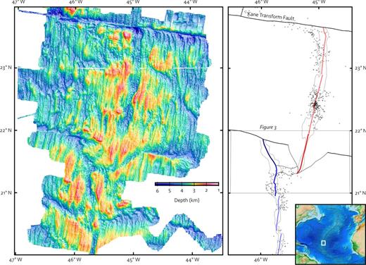
Location map showing regional bathymetry (left) and an outline of the rift geometry (right) with features related to the TAMMAR propagating segment highlighted (refer to cartoon in Fig. 1). The box indicates the coverage of the detailed map in Fig. 3. Also on the right is seismicity (circles) from Smith et al. (2003) with only those events with picks on at least five stations shown. The inset map (bottom right) gives an overview of the study location in the North Atlantic Ocean.

Open in new tabDownload slide

Here, we follow the nomenclature proposed by Hey et al. (1986) to describe the geomorphological features of a propagating rift system. Hey et al. (1980) first outlined the geometry of such a system and the geometry and kinematics were mathematically described by McKenzie (1982, 1986). This is summarised in Fig. 1(a). The propagating rift extends at the expense of the doomed rift, which becomes the failed rift once spreading ceases. The transition of spreading from the doomed rift to the propagating rift takes place over a finite distance, resulting in a transform zone between the two segment ends in which material is sheared as it transitions from one tectonic plate to the other. Material that has passed through the transform zone remains indefinitely in the sheared zone thereafter. Inner and outer pseudo-faults separate material created at the propagating rift and material created at the doomed rift.

The broad-scale general tectonics of the section of the Mid-Atlantic Ridge between 20°N and 24°N has been investigated extensively through the use of gravity, magnetic and bathymetric data (Gente et al.1995; Pockalny et al.1996; Maia & Gente 1998; Ravilly et al.1998), unravelling a complex migration history of second- and third-order ridge discontinuities. Maia & Gente (1998) carried out modelling of shipboard gravity to estimate crustal thickness in the region, and identified a mantle Bouguer anomaly associated with a maximum in the long-wavelength bathymetry centred directly on the TAMMAR segment. They attributed this as marking the site of a possible mantle upwelling. In this paper, we apply their method, with some modification, to satellite altimetry-derived gravity data in order to investigate in detail the kinematics of the TAMMAR region and extrapolate the seismic refraction results across the sheared zone.

Fig. 3 shows the detailed morphology of the TAMMAR propagating system. The pseudo-faults enclose the propagating rift in a clear ‘V’ which ends abruptly at a fossil fracture zone. From the length of the fracture zone, it is clear that the discontinuity was a stable transform offset for at least 10 Myr before the onset of propagation (Fig. 2). Similarly, we can deduce that propagation commenced at 3.5 Ma. The propagating segment has a narrow, well-defined, hourglass-shaped axial valley with relatively small, closely spaced abyssal hills, indicative of mainly magmatic spreading. This observation is supported by the presence of numerous small hummocks assumed to be volcanic in origin, as well as an almost complete lack of seismicity in the propagating rift (Smith et al.2003).

Figure 3.

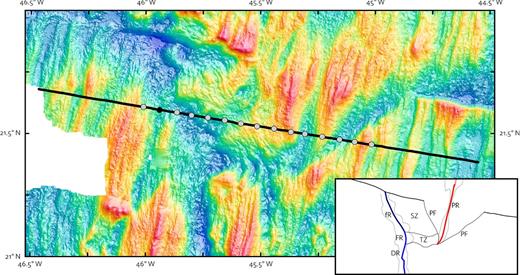
Detailed bathymetry map of the propagating rift system including seismic refraction line. Circles represent OBH stations. The stations are numbered sequentially from east to west, running from OBH16 through to OBH30. OBH29 (black) did not record any data. Shots were fired approximately every 120 m along the black line. The bathymetry colour scale is as in Fig. 2. Inset is a sketch of the main tectonic elements with abbreviated annotations as in Fig. 1. The propagating rift is framed by an obvious ‘V’ formed by the inner and outer pseudo-faults. It has a well-defined, narrow axial valley, reflecting that magmatism plays an important role in its spreading. The doomed rift, on the other hand, has a broad, asymmetric axial valley. Crust is clearly seen to deform severely as it passes through the transform zone into the sheared zone.

Open in new tabDownload slide

In contrast, the doomed rift is extremely seismically active (one of the ‘seismic stripes’ recognised in Smith et al.2003) and has a broad and asymmetric morphology with a poorly defined axial centre. A large part of the spreading in the doomed rift is therefore assumed to be taken up by normal faulting. Buck et al. (2005) provide an excellent explanation of the link between magmatic spreading fraction and abyssal hill morphology.

The offset between the propagating and doomed rifts is about 40 km. The straight line of the outer pseudo-fault indicates that the propagation rate has been constant since its onset, and the angle between the pseudo-fault and the ridge axis implies a propagation rate of 14 km Myr⁻¹, or 15 per cent faster than the half-spreading rate. The bathymetric map clearly shows how the fabric of the seafloor deforms as it passes through the transform zone into the sheared zone (Fig. 3).

Dannowski et al. (2011) carried out tomographic inversion on a seismic line along the axis of the propagating rift. They confirm increased magmatism at the propagating rift and propose that melt is channelled towards the ridge-tip, and that this is related to the mechanism of propagation. They go on to propose a localised mantle upwelling, in agreement with Maia & Gente (1998), and state that this is the likely ultimate cause of the propagation of the TAMMAR ridge segment.

This explanation may well be correct, but we still have no concrete foundation on which to build an understanding of rift propagation. Since rifting is a passive process, ultimately driven by stresses and failure, it seems likely that lithospheric strength, deformation processes and localised stresses must play an important role. Attention must therefore be focused on these in order to build a picture of the dynamics of the system. Many of these stresses and their resulting deformation play out in the transform zone. In this paper, we focus on a seismic refraction line across the propagating rift, sheared zone and failed rift in order to understand the kinematics of deformation in the transform zone. This understanding of the kinematics of propagation is a necessary precursor to understanding the dynamics of the system.

2 SEISMIC REFRACTION TRAVELTIME INVERSION

This section deals with the processing and inversion of a 200 km long seismic refraction line across the propagating rift system, spanning the outer pseudo-fault, propagating rift, inner pseudo-fault, sheared zone and failed rift (Fig. 3). Airgun shots were fired approximately every 120 m along the line. Fifteen ocean bottom hydrophones, evenly spaced along the central 100 km of the refraction line, recorded the shots at 100 or 125 data samples per second (depending on the station). The hydrophone stations were labelled OBH16–30 incrementally from east to west. OBH29 failed to record any data.

2.1 Clock drift

Each instrument was deployed for about 50 hr. The instrument clocks were synchronised to GPS time on deployment and retrieval; we corrected any clock drift by linear interpolation. Clock drifts ranged from −11 to 13 ms with an rms value of 6.3 ms, and were therefore insignificant relative to the estimated traveltime pick error.

2.2 Station relocation

Because each hydrophone can be carried by currents in the water column as it descends from the ship to the seafloor, exact instrument locations are not accurately known. We estimated instrument locations along the seismic line by fitting a hyperbola to the direct (water wave) arrival for each station; we picked the direct arrival by hand and used cross-correlation between traces to improve the accuracy and consistency of the picks. We made no attempt to estimate any off-axis location error. All but one station (OBH19) had an along-line location error of less than twice the shot spacing.

We also used the best fit of the direct arrival hyperbolæ to a uniform velocity model to calculate the average acoustic velocity of the water column (1.510 km s⁻¹), as well as a static timing correction (−1.60 s) that needed to be applied to the seismic traces.

Finally, the hyperbolæ can be used to estimate station depths. Although we used the bathymetry to set station depths, it is encouraging that these depths agree with those calculated from the direct arrival hyperbolæ with a standard error of under 30 m (median error of 18 m and maximum disagreement of 53 m, station OBH17).

2.3 Data quality and traveltime picks

Fig. 4(a) shows an example of the recorded raw data. The data show strong ringing due to bubble pulses, making identification of seismic phases (in particular PmP) difficult. We used the blind deconvolution method of Bell & Sejnowski (1995) to remove the ringing effect from the data. This method takes an information maximisation approach to estimating an optimal linear deconvolution filter. We determined deconvolution filters of length two seconds for each hydrophone station. Training data sets for each station were made up of 100 000 randomly chosen time-series of length 1000 samples from traces with an offset of at most 20 km from the corresponding station. The results are shown in Fig. 4(b)—there is a marked improvement in data quality and the PmP arrival is much clearer. Fig. S1 in the Supporting Information shows the optimal deconvolution filters, as well as their inverse (the recovered source wavelet).

Figure 4.

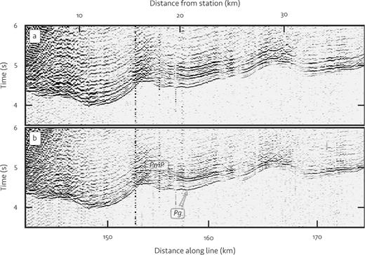
Improvement of data quality by deconvolution, illustrated with part of the record section for station OBH18. Data are shown before (a) and after (b) deconvolution. Strong ringing due to bubble pulses obscures the PmP arrival in (a). The ringing is characteristic for all stations and is largely removed during deconvolution (b). The data are shown high-pass filtered at 10 Hz and plotted with a reduction velocity of 8 km s⁻¹.

Open in new tabDownload slide

We picked first arrival Pg and Pn traveltimes wherever possible, as well as the PmP reflected arrival wherever it was clear and unambiguous. In general, the PmP arrival was very weak and difficult to pick beneath the sheared zone and doomed rift, and was clearest in the easternmost part of the refraction line. This is discussed in more detail in Section 7.

The standard error of the direct (water wave) traveltime picks (see above) as estimated by cross-correlation between traces was 0.02 s. Since the direct arrivals are typically much stronger than the refracted first arrivals, we estimate the first arrival pick error to be around 0.05 s and the weaker PmP arrival pick error to be 0.10 s.

The full set of record sections and picks is shown in Fig. S2 in the Supporting Information.

2.4 Starting model

For the starting model, we determined the 1-D velocity model that best fits the first arrival traveltime data for all stations. We did this by minimising the L_1.5-norm of the data residual together with a regularisation term minimising the integral |$\int _0^{z_{\rm max}} \left| \frac{\partial v}{\partial z} \right| dz$|⁠. The velocity model is parametrised as a (smooth) B-spline with six nodes. We corrected for bathymetric effects by projecting a ray from each shotpoint to the seafloor. We determined the angle of the ray using the ray parameter ∂t/∂x (horizontal slowness) and the water column acoustic velocity. The length of the ray determines the bathymetric traveltime correction, while the intersection point on the seafloor determines the bathymetry-corrected offset.

Figure 5.

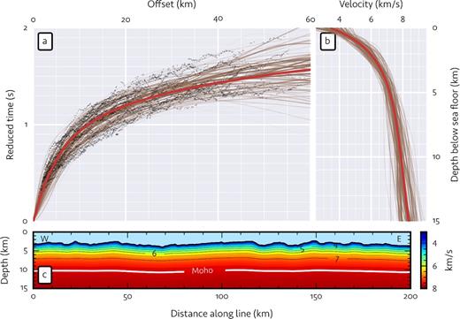
Starting model. Part (a) shows the bathymetry-corrected first arrival traveltimes (dark points) plotted against offset. A reduction velocity of 8 km s⁻¹ is used. The thick red line shows synthetic traveltimes for the best-fitting 1-D velocity model (b). The faint brown lines in both (a) and (b) show equivalent plots for the Monte Carlo starting models. The weight of these lines indicates qualitatively how well each starting model fits the bathymetry-corrected traveltime data. The 2-D starting velocity model constructed from the best-fitting 1-D model using eq. (1) is shown in (c) with a vertical exaggeration of 2:1.

Open in new tabDownload slide

2.5 Inversion parameters and traveltime inversion

We inverted the first arrival traveltimes and PmP reflections for the best-fitting velocity model using the software Tomo2D (Korenaga et al.2000). Tomo2D jointly inverts for first arrival refracted traveltimes as well as reflected traveltimes to constrain a single, floating reflector (the Moho in this case) within the velocity model.

Tomo2D parametrises the velocity model as a set of grid nodes hanging from the bathymetry. We used a constant horizontal grid spacing of 400 m and a variable vertical grid spacing ranging from under 50 m at the seafloor to 200 m at a depth of 15 km below the seafloor. Tomo2D allows horizontal and vertical length scales to be set over which velocity perturbations are assumed to be correlated. These correlation lengths prevent unresolvable velocity changes and oscillations from appearing in the final model. We chose correlation lengths based on the heuristic argument outlined below.

It is reasonable to assume that velocity perturbations are primarily determined by horizontal (turning) rays, since relative traveltime calculations (or, more specifically, the gradient of traveltime with offset) are dominated by the velocity at the turning point. Under this assumption, the vertical correlation length will be determined by the width of the first Fresnel zone, while the horizontal correlation length will be determined by the station spacing (due to smearing effects). We therefore set the horizontal correlation length to 7 km (approximately the station spacing) and the vertical correlation length to an estimate of the width of the first Fresnel zone at each point.

The first Fresnel zone for a given wavelength λ is |$F_1 \approx \sqrt{\lambda \, d_1 d_2 / \left( d_1 + d_2 \right)}$|⁠, where d₁ is the ray distance to the receiver and d₂ is the ray distance from the source. This value is maximal at the midpoint, where d₂ ≈ d₁, consequently |$F_1 \lesssim \sqrt{\lambda \,d_1 / 2}$|⁠. For each station, a conservative estimate of the Fresnel zone at each point in the model can therefore be calculated using this upper bound. We set the vertical correlation length at each point to the weighted mean of this estimate for each station. The estimates were weighted by the inverse of the square of the station distance. The wavelength was determined for a wave of frequency 10 Hz using the velocities of the starting model. This scheme results in vertical correlation lengths of around 200 m near stations increasing to 2 km near the Moho and almost 3 km at the base of the model (15 km below the seafloor).

Tomo2D also allows separate velocity and reflector smoothing weights to be specified for further regularisation of the model. We chose velocity and depth smoothing weights of 150 and 20, respectively, by considering L-curves derived from single inversion iterations at a range of smoothing weights.

We carried out 100 inversion iterations to construct the final velocity model (Fig. 6a) with a χ² fit of 1.3 and an rms traveltime misfit of 0.06 s. The crustal χ² fit and rms misfit are 1.5 and 0.06 s, respectively; the corresponding PmP values are 0.2 and 0.05 s.

Figure 6.

Final P-wave velocity model (a) and chequerboard resolution tests (c)–(e). Part (b) shows the velocity anomalies added to (a) for the chequerboard test. In (c), chequerboard test is noise-free, that is, the synthetic traveltimes are unperturbed. In (d), the synthetic traveltimes are perturbed by random Gaussian noise with a standard deviation of 50 ms, and in (e) they are perturbed by the actual data residual. The profiles are plotted with a vertical exaggeration of 2:1. The thick white lines in (a), (c), (d) and (e) show the Moho as imaged in the tomographic inversion. The red and blue filled regions in (c), (d) and (e) show where the recovered Moho for the chequerboard tests is shallower and deeper, respectively, than in (a). The Moho perturbations are exaggerated by a factor of four for clarity. In panels (a), (c), (d) and (e), the models have been masked based on the derivative weight sum (DWS) so that only those areas that are constrained by the data are shown. The logarithm of the DWS is shown in (f). Part (g) shows the velocity standard deviation of the Monte Carlo simulation.

Open in new tabDownload slide

2.6 Resolution tests

We carried out chequerboard resolution tests using the method outlined below. We added alternating sinusoidal velocity perturbations to the final model (Fig. 6b), with horizontal width (half-wavelength) 10 km, vertical height (half-wavelength) 4 km and amplitude 0.1 km s⁻¹. The small amplitude (about 3 per cent of the lowest velocities in the final model) ensures that ray paths are not materially affected by the perturbations. We then calculated synthetic traveltimes at all pick locations for the perturbed velocity model. Finally, we inverted the adjusted traveltime picks following the same procedure as described in 2.5 above, starting with the original starting model, and compared the resulting velocity model with the final model in Fig. 6(a).

The results of this noise-free chequerboard test are shown in Fig. 6(c). Within the part of the profile occupied by stations, the perturbations are well resolved in the upper crust, both in amplitude and shape; in the lower crust, the amplitudes are still reproduced, but the perturbation edges are distorted due to smearing effects. In the eastern and western parts of the profile not occupied by stations, the perturbations are much less well resolved, being extensively smeared along the ray paths. This suggests that the final model is only trustworthy within the region occupied by stations, and that structures at depth may be distorted by smearing. Anomalies roughly the size of the velocity perturbations are expected to be robust.

We also carried out two perturbed chequerboard tests. In the first (Fig. 6d), we added random Gaussian noise with a standard deviation of 50 ms to the synthetic traveltimes. The recovered pattern and amplitude is very similar to the noise-free test, with a small loss of resolution.

In the second perturbed chequerboard test (Fig. 6e), we added the actual data residuals to the synthetic traveltimes. In this case, the recovered pattern is very similar to the noise-free test, but the amplitudes of the velocity perturbations were not well recovered. This can be understood because the traveltime changes due to the minor chequerboard velocity perturbations are small compared to the expected pick error of 0.05 s. The result is to exaggerate the effect of traveltime mispicks.

Also shown in Figs 6(c)–(e) is the discrepancy between the Moho recovered in the chequerboard tests and that recovered in the original inversion. In the figure, this is exaggerated by a factor of four for clarity. In the noise-free test, the Moho discrepancies are so small as to be nearly invisible. This gives us good confidence that there is little trade-off between anomaly recovery and imaged Moho depth. In both perturbed tests, however, the Moho discrepancies are much larger, up to about 600 m. Errors in the traveltime data therefore have a far greater effect on imaged Moho depth.

2.7 Model robustness

We estimated the robustness of the velocity model by carrying out a Monte Carlo simulation using 100 different starting models. The variation in the final velocity models of the ensemble gives an indication of the uniqueness of the solution.

We constructed the starting models by creating 100 random 1-D models that fit the bathymetry-corrected traveltime data to within twice the misfit of the original best-fitting 1-D model. The random models were generated by repeatedly changing both the B-spline node velocity values as well as the inner node locations by uncorrelated random perturbations (normally distributed with standard deviations of 1 km s⁻¹ and 1 km for the velocities and locations, respectively) and selecting the first 100 that fit the data to within the threshold. We then constructed the 2-D starting models using the same procedure as in Section 2.4. The 1-D models are plotted in Fig. 5(b), with the synthetic traveltimes shown in Fig. 5(a).

For each starting model, we carried out a full inversion following the procedure in Section 2.5. Fig. 6(g) shows the velocity standard deviations of the 100 final models. Most of the model space has a standard deviation below 0.2 km s⁻¹, although this increases in the shallow crust.

3 GRAVITY MODELLING

We estimated crustal thickness variation using the satellite altimetry-derived free air gravity from Sandwell et al. (2014) and updated bathymetry from Smith & Sandwell (1997). We used densities of 1.0, 2.9 and 3.3 g cm⁻³ for sea water, oceanic crust and mantle, respectively. The calculation comprised the following steps, illustrated in Fig. 7:

• The Bouguer correction due to the bathymetry was determined using the method of Parker (1973).

• Thermal subsidence was estimated from the bathymetry using a median filter with a window size of 100 km and converted to the equivalent Bouguer anomaly (Fig. 7b).

• The Bouguer correction was adjusted by subtracting the thermal subsidence contribution estimated in step (ii) (i.e. the thermal subsidence height multiplied by the gravitational constant and the density difference between crust and sea water; the results are shown in Fig. 7c).

• The residual Bouguer gravity was downward-continued by 10 km (the approximate depth of the Moho below sea level near the ridge axis) to reduce errors introduced by the 1-D approximation in step (viii).

• Spurious short-wavelength features in the residual Bouguer gravity were removed using a low-pass filter with a cut-off wavelength of 7.5 km.

• Very long-wavelength deep-seated gravity variations were removed using a high-pass filter with a cut-off wavelength of 750 km.

• Oscillations due to the sharp cut-off in step (v) were removed using a Gaussian filter with one standard deviation width 7.5 km.

• Moho depth perturbations were estimated using the 1-D Bouguer approximation.

• Crustal thickness perturbations were estimated by subtracting the bathymetry (smoothed using a Gaussian filter to match step (vii)) and removing the median value (Fig. 7d).

Figure 7.

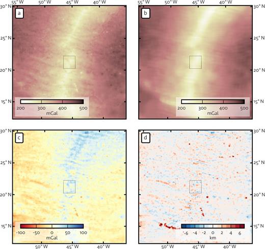
Steps in modelling crustal thickness from gravity, showing the (a) Bouguer anomaly, (b) contribution due to thermal subsidence, (c) Bouguer anomaly corrected for thermal subsidence and (d) estimated crustal thickness anomaly. We calculate (c) by subtracting (b) from (a). Note the residual long-wavelength anomaly. We assume this to be of deep mantle origin and remove it using a high-pass filter before conversion to crustal thickness (step (vi) in the text). The rectangle in the centre of each map indicates the study area.

Open in new tabDownload slide

Our calculations broadly follow Maia & Gente (1998), but differ primarily in the method of estimating thermal subsidence; Maia & Gente (1998) use a high-pass filter to remove thermal subsidence effects, whereas we apply a median filter to the bathymetry to estimate thermal subsidence, and then remove its effect. We found the approach using a high-pass filter to be unsatisfactory since it was not robust (i.e. results were highly dependent on the choice of cut-off wavelength for the high-pass filter). Results using the median-filter approach, on the other hand, were minimally affected by the choice of window size except at the limit of small windows.

4 CRUSTAL STRUCTURE

Fig. 8 summarises the results of the seismic tomographic inversion and gravity modelling. The depth variations in the Moho reflector modelled in the tomographic inversion very closely match those determined by gravity modelling. The agreement of these independent but complementary methods gives additional confidence in the results.

Figure 8.

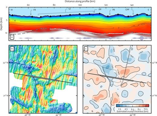
Crustal structure from seismic refraction and gravity. Part (a) shows a detailed view of the seismic refraction model, covering only the section of the profile which is well resolved. The failed rift (FR), sheared zone (SZ), propagating rift (PR) and pseudo-faults (IPF/OPF) are marked. The Moho as modelled from gravity is plotted as a dashed line. This is based on an average crustal thickness of 6.5 km, which gives a good fit to the seismic Moho. The profile is plotted with a vertical exaggeration of 2:1. The light grey violin plot at the base indicates the relative density of PmP picks located at their modelled reflection point on the Moho. Part (b) shows a bathymetric map (colour scale as in Fig. 2) indicating the seismic line with the plotted section highlighted. Part (c) shows a map of the crustal thickness anomaly as modelled from gravity. The filled contours represent intervals of 1 km. The colour bar shows the estimated crustal thickness values based on a good fit with the seismic inversion (i.e. using an average crustal thickness of 6.5 km).

Open in new tabDownload slide

We used an average crustal thickness of 6.5 km for plotting the Moho as modelled from gravity, since this value gives the best agreement with the seismic refraction results (the gravity modelling estimates only perturbations to the crustal thickness or Moho depth). We therefore take 6.5 km to be the average crustal thickness in all discussions that follow. This is within the limits of ‘average oceanic crust’ (7.1 ± 0.8 km) as observed globally by White et al. (1992), albeit on the thin side.

The seismic velocity structure conforms to typical oceanic crust, with a steep velocity gradient up to about the 6–6.5 km s⁻¹ contour (seismic Layer 2, upper 1.5 km), followed by a gentle gradient to the base of the crust (seismic Layer 3). However, Layer 3 appears to be extremely thin beneath the failed rift and the western part of the sheared zone, resulting in a thin crust of under 5 km. In contrast, the crust formed by the propagating rift reaches a maximum thickness of almost 8 km and is in very good agreement with the along-axis refraction survey of Dannowski et al. (2011).

This pattern is echoed by the gravity-derived crustal thickness map. The crust produced by the propagating rift is everywhere anomalously thick, except near the outer pseudo-fault where the bathymetry is particularly deep (reaching 4 km). At its centre, this section of crust reaches a maximum thickness which is more than 2 km greater than average crust (or about 9 km for an average crustal thickness of 6.5 km).

In sharp contrast, the sheared zone and failed rift are mostly made up of particularly thin crust (more than 1 km thinner than average). The crust in this region reaches its thinnest point in the NW corner of the sheared zone, 3 km thinner than average (or only about 3.5 km thick). This coincides with a deep bathymetric basin (over 6 km deep).

The juxtaposition of anomalously thick crust formed at the propagating segment next to particularly thin crust in the sheared zone calls for some consideration. The thick crust of the propagating segment is suggestive of increased magmatism; indeed, this proposal is well supported by the smooth hummocky bathymetric morphology indicating dominant volcanic activity. The lack of seismicity (see Fig. 2) along the propagating segment is further evidence for predominantly magmatic spreading.

The thin crust in the sheared zone and failed rift is perhaps less obviously explained. It is possible that this could be related to poor magma supply to the doomed and failing rift. Elsewhere (e.g. Minshull et al.2006), thinning in Layer 3 has been associated with reduced magma supply. This explanation would be consistent with the high levels of seismicity along the doomed rift (Smith et al.2003). However, it does not explain the thick crust observed in the gravity model to the west of the failed rift. We therefore suggest that any explanation is likely to relate to the extreme deformation that takes place in the transform zone. We discuss possible deformation kinematics and the implications thereof in detail in Section 5.

5 TRANSFORM ZONE KINEMATICS

Figure 9.

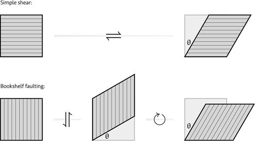
Simple shear and bookshelf faulting model. The top panel shows right lateral simple shear by an angle θ. The bookshelf faulting model (bottom) for shear of the same angle can be deconstructed into left lateral simple shear and clockwise rotation. Although the same angle of shear results, the final body is laterally extended and vertically shortened in comparison to the simple shear case.

Open in new tabDownload slide

It is clear from Fig. 9 that the final deformation resulting from bookshelf faulting is not identical to that of simple shear. For any given angle θ of shear, bookshelf faulting shortens the body in the vertical (ridge-parallel) direction and extends it in the horizontal (transform-parallel) direction. This suggests an attractive hypothesis for explaining the thin crust in the sheared zone: in order to counter the ridge-parallel shortening imposed by bookshelf faulting, the crust may be forced to thin. The transform-parallel extension, on the other hand, could be accommodated simply by reducing the half-spreading rate within the transform zone accordingly (i.e. the extension could contribute to plate spreading).

But do the numbers add up? In the discussion below, we estimate that at most 60 per cent of the shear can be taken up by slip on reactivated normal faults. The remainder must be accommodated by a different mechanism.

If we assume that all of the shear is accommodated by bookshelf faulting, this analysis has two implications. The first is that, to overcome the ridge-parallel contraction, the crust must thin to about half its original thickness, or about 3–3.5 km for ordinary crust. This would necessarily require the creation of new normal faults. Although there may be some crust as thin as this in the sheared zone (see Fig. 8c), the majority of it falls in the range 4.5–6.5 km.

The second implication is that the final width of the sheared zone must be about double the width of the material entering the transform zone. This is clearly not the case, and would be kinematically difficult to achieve.

Evidently, neither of these implications is observed in the TAMMAR propagating system. On average, the transform-parallel distance between the inner pseudo-fault and the propagating rift axis is about 9 km less than the distance between the outer pseudo-fault and the rift axis. The offset between the propagating and doomed rifts is about 40 km. If the 9 km discrepancy is a result of extension during bookshelf faulting, this would suggest a total shear angle due to bookshelf faulting of |$\theta = \arccos \left({{\rm 40}}/{{\rm 49}} \right) \approx {35^{\circ }}$|⁠. Similarly, if bookshelf faulting thinned the crust in the sheared zone to its average of around 5.5 km from an original thickness of 6.5 km, the total shear angle due to bookshelf faulting would be |$\theta = \arccos \left({{\rm 5.5}}/{{\rm 6.5}} \right) \approx {32^{\circ }}$|⁠. These angles are in good agreement and suggest that only about 40 per cent of the necessary shear may be taken up by bookshelf faulting since tan 35° ≈ 0.7 ≈ 0.4 γ.

So far we have only considered reactivation of normal faults in a strike-slip sense. If we allow an arbitrary slip vector for the reactivated faults, could the difficulties above be overcome? Could a component of thrusting on the reactivated normal faults act both to thicken the crust and reduce the final width of the sheared zone?

We can now use |$\mathbf {\tilde{B}}$| to estimate how the introduction of thrusting might affect the discussion above. If we assume reasonable limits of: (1) an original dip ψ₁ = 45° on normal faults; (2) a final maximum dip of 60° after thrusting (i.e. ψ₂ < 60° since the final angle of dip is greater than ψ₂), we still find that our modified bookshelf faulting can account for no more than 60 per cent of the shear (⁠|$\theta \lesssim \arccos \left({\left(\cos {35^{\circ }}\,\sin {45^{\circ }}\right)}/{\sin {60^{\circ }}} \right) \approx {45^{\circ }}$|⁠; tan θ ≈ 1 ≈ 0.6 γ).

If all shear deformation were to be taken up by slip on reactivated normal faults, |$\mathbf {\tilde{B}}$| would require the original dip for the normal faults to be bounded by |$\psi _1 \lesssim \arcsin \left({\sin \psi _2\,\cos \theta }/{\cos {35^{\circ }}} \right) \approx {30^{\circ }}$|⁠. This is very much an upper bound since, for such large θ, ψ₂ is unlikely to reach 60°. Indeed, if the final angle of dip is 60°, ψ₂ would be only about 40°, with ψ₁ ≲ 23°. This bound implies unrealistically shallow original angles of dip.

The crustal thinning required by the bookshelf faulting model necessarily requires new normal faults to be created. These faults then have the potential to fail in a strike-slip sense to take up shear deformation. We therefore propose that the required shear deformation in the transform zone is partitioned between bookshelf faulting and simple shear. Furthermore, this partitioning is patchy, resulting in bookshelf-faulted blocks separated by thinned crust which has undergone simple shear. This is consistent with the uneven crustal thickness and bathymetry in the sheared zone and the crooked inner pseudo-fault and crooked inner boundary of the failed rift.

6 STRUCTURAL ORIENTATIONS IN THE SHEARED ZONE

We can investigate the arguments above by examining structural features in the bathymetry of the sheared zone. Fig. 10 shows two superimposed rose diagrams giving structural orientations automatically extracted from a high-pass filtered version of the bathymetry. The rose diagrams represent a weighted distribution of structural correlations at 25 000 evenly spaced points in the sheared zone. We use correlations of parallel profiles to infer orientations of continuous structural features. At each point, we determine structural correlations as follows:

• For each azimuth, we extract bathymetry along four pairs of parallel profiles oriented perpendicular to the azimuth. We choose profile pairs equidistant from the point and separated by 200, 400, 600 and 800 m, respectively.

• For the ith profile pair |$\left(p^i_1, p^i_2\right)$|⁠, we calculate a correlation coefficient Cⁱ using a Gaussian weighting function w with FWHM of 2.5 km. Cⁱ is given by

  \begin{equation*} C^i = \frac{\sum _k{w_k^2\,p^i_{1k}\,p^i_{2k}}}{\sqrt{\sum _k{\left(w_k\,p^i_{1k}\right)^2}\sum _k{\left(w_k\,p^i_{2k}\right)^2}}}{\rm .} \end{equation*}

• We take the mean of the four coefficients as the final correlation coefficient C for each azimuth.

Figure 10.

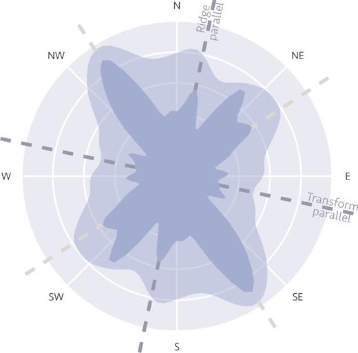
Structural orientations in the sheared zone determined from bathymetric morphology. Dark broken lines show ridge-parallel and transform-parallel directions; pale broken lines lie 45° from ridge-parallel and transform-parallel directions. The main structural orientation, representing rotated abyssal hills, lies 45° counter-clockwise of the ridge-parallel direction. There is a secondary structural orientation from 30° to 45° clockwise of the ridge-parallel direction. Section 6 describes the method for constructing the rose diagrams. The lighter rose diagram uses all positive structural correlations, while the darker diagram uses only those correlations greater than 1/2.

Open in new tabDownload slide

The lighter rose diagram in Fig. 10 shows the distribution of all positive structural correlations weighted by the square of the correlation coefficient C. We use the square of C as a weighting to select for orientations showing strong correlation. The darker rose diagram weights strong correlations even higher. It shows the distribution of only those correlations with coefficients C > 1/2, weighted by (C − 1/2)².

The major structural orientation corresponds to rotated abyssal hills and is almost exactly 45° counter-clockwise of the ridge-parallel direction. The width of the sheared zone, its crustal thickness and the orientation of its fabric are therefore all in excellent agreement with each other in the context of the model presented in Section 5. These observations suggest that the thinned crust in the sheared zone can be explained if deformation in the transform zone is taken up along reactivated normal faults, but that slip on pre-existing faults takes up no more than 60 per cent of the required shear in the transform zone.

There is a secondary structural orientation in Fig. 10 between 30° and 45° clockwise of the ridge-parallel direction. This secondary orientation may represent new normal faults formed to accommodate the crustal thinning required by bookshelf faulting.

7 SERPENTINISATION BENEATH THE SHEARED ZONE

Figure 11.

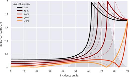
Amplitude of PmP reflection coefficient with angle of incidence for varying degrees of serpentinisation. The thin lines show intermediate degrees of serpentinisation between the thick lines labelled in the legend. For serpentinisation as low as 25–30 per cent, the reflection coefficient becomes insignificant except at very high angles of incidence where the PmP arrival is indistinguishable from the direct arrival. This effectively demonstrates how even low levels of serpentinisation can result in no obvious PmP in the record section, as is observed under most of the sheared zone and doomed rift. The filled grey region in the background indicates the distribution of angles of incidence for all PmP picks as given by the ray paths in the tomographic inversion. This coincides very well with the critical angle for normal crust overlying unaltered mantle.

Open in new tabDownload slide

Although serpentinisation may effectively remove the PmP arrival, there must of course still be a transition from serpentinised to unserpentinised mantle. If this transition takes the form of a sharp front, one could expect high-amplitude reflections from the serpentinisation front. However, it is more likely that the transition is gradual, and if it extends over sufficient distance (about half a wavelength, ∼500 m) there will be no reflection.

The low density of serpentinised peridotite raises questions about the crustal thickness model based on satellite-altimetry gravity data; the model will overestimate crustal thickness where a layer of serpentinised mantle is present. However, this effect is minor. A 1 km thick layer of 20–25 per cent serpentinised mantle (density about 3.1 g cm⁻³) would result in a crustal thickness overestimate of only a few hundred metres. This is small compared to errors due to oversimplification of the model, for instance, the assumed uniform crustal density.

8 CONCLUSIONS

This study has clarified many details of the kinematics of the TAMMAR propagating rift system, a rare example of a true propagating rift, whose tip must break into older and stronger lithosphere.

The fossil fracture zone confirms that a stable transform offset existed for at least 10 Myr before the onset of propagation. At about 3.5 Ma, the offset lost its stability and southward propagation began. It is unclear what the trigger for this was, but the angle and continuity of the outer pseudo-fault indicates that propagation has continued at a constant rate of about 14 mm yr⁻¹ (15 per cent faster than the half-spreading rate) for the history of the system.

We have shown that the crust within the sheared zone is on average over 1 km thinner than normal. Thin crust is expected if the required shear in the transform zone is taken up by reactivation of pre-existing normal faults in a strike-slip sense (bookshelf faulting). However, the bookshelf faulting model predicts far greater crustal thinning than is observed, forcing the conclusion that at most 60 per cent of the required shear deformation within the transform zone can be explained by reactivation of pre-existing faults. This conclusion is supported by the width of the sheared zone relative to the transform zone, as well as the angle of rotation of the abyssal hills within the sheared zone.

The crustal thinning required by the bookshelf faulting model necessarily requires new faults to be created. We propose that the required shear deformation in the transform zone is partitioned between bookshelf faulting along pre-existing normal faults and simple shear along newly created faults.

The extensive faulting and fracturing in the sheared zone may have allowed sufficient hydrothermal circulation to serpentinise the mantle beneath the Moho. We show that moderate serpentinisation (25–30 per cent) is sufficient to remove any observable PmP reflection. Serpentinisation of the mantle may therefore explain the weak or absent PmP arrivals in the sheared zone, particularly in the west where the crust is thinner, suggesting effective transport of hydrothermal fluids through the sheared zone crust.

Some of this work was carried out as part of a PhD dissertation at the University of Cambridge. This project was funded by the German Science Foundation (DFG grants Mo 961/5-1 and Gr 1964/8-2+8-3); RLK was supported by a Cambridge Mandela Scholarship and by the German Academic Exchange Service (DAAD). The authors would like to thank the captain, crew and scientists of F/S Meteor on cruise M60/2. Jason Phipps Morgan, César Ranero, Márcia Maia and Pascal Gente offered guidance on the cruise and made their bathymetric data available; we are also grateful to Bob White, Tim Reston, Beth Kahle and Alastair Sloan, as well as the reviewers, Tim Minshull and anonymous, for their helpful comments and suggestions. Figures were prepared using the Python modules Matplotlib and Basemap.

REFERENCES

SUPPORTING INFORMATION

Additional Supporting Information may be found in the online version of this paper:

Figure S1. (a) The deconvolution filter and (b) recovered source-time function for each record section as estimated by the information maximisation approach of Bell & Sejnowski (1995). The bubble pulses of the source-time function appear to be somewhat different at the far western end of the line, resulting in unsatisfactory deconvolution and recovery for station OBH30.

Figure S2. Record sections for stations OBH16–20 with (bottom) and without (top) traveltime picks (red) and synthetic traveltimes (black). Data are shown after deconvolution and bandpass filtered between 7 and 30 Hz. A reduction velocity of 8 km s⁻¹ is used.

(Supplementary Data).

Please note: Oxford University Press is not responsible for the content or functionality of any supporting materials supplied by the authors. Any queries (other than missing material) should be directed to the corresponding author for the paper.