


Abstract
Inhomogeneous noise sources surrounding stations produce asymmetric amplitudes in cross-correlation functions that yield preferential source directions. Here we show that preprocessing biases the dominant source direction estimate towards the source producing long-duration signals by down-weighting high-amplitude signals. Tests with both synthetic data and observations show that conventional preprocessing, where only earthquakes and local transients (e.g. trawling, fish impacts) are removed, is more sensitive to coherent energy, while one-bit preprocessing and running-absolute-mean preprocessing are more influenced by signal duration. Comparisons between different preprocessing methods are made on data from the Cascadia Initiative ocean bottom seismometer array, where we find that the total energy arriving from pelagic and coastal areas is similar. Moreover, pelagic-generated signals tend to be weaker but have longer duration, in contrast to coastal-generated signals that tend to be stronger but have shorter duration.
1 INTRODUCTION
Conventional seismic tomography has been extensively used to study the Earth's structure, see reviews by Romanowicz (1991, 2003). However, as earthquake sources are spatially restricted, the more widely distributed ambient noise sources provide another important resource to study Earth structure. It has been demonstrated that Green's functions can be extracted from the ambient noise cross-correlation functions (Snieder 2004; Sato & Fehler 2009), which became the foundation of ambient noise tomography. However, the reliability of the extracted Green's functions depends on the validity of the assumption that the noise sources are homogeneously distributed. Although seismic data preprocessing, especially one-bit and running absolute mean (RAM), serves to better spatially homogenize the noise field that allows unbiased estimates of traveltimes (Shapiro et al.2005; Harmon et al.2010) and usually increases signal-to-noise ratio (SNR) for surface waves, absolute amplitude information is lost. Besides, ambient noise has also been used for crustal attenuation estimation (e.g. Prieto et al.2009; Lin et al.2012). However, noise source distribution has an effect on the coherency amplitude decay rate with station separation, which is important for attenuation coefficient estimation (Tsai 2011). Therefore, it is important to study the distribution of noise sources to investigate whether a homogeneous source distribution assumption is valid, and to determine the impact on cross-correlation functions if it is not (Yao & Van der Hilst 2009; Cupillard & Capdeville 2010; Harmon et al.2010).
Microseisms (0.05–0.35 Hz) have been studied for several decades, with the dominant source area of double-frequency (DF) microseisms (0.1–0.35 Hz) an important but unresolved issue (Bromirski et al.2013). It is generally accepted that single-frequency (SF) microseisms (0.05–0.1 Hz) are generated by the interaction between the ocean waves and the seafloor near coasts (Hasselmann 1963), while DF microseisms are generated by counter-propagating, or more generally, obliquely interacting surface waves (Longuet-Higgins 1950; Traer & Gerstoft 2014). For the SF band, all studies support shallow water generation (Cessaro 1994; Bromirski & Duennebier 2002), consistent with the theoretical work by Hasselmann (1963). For the DF band, however, both pelagic generation (Bromirski et al.2005; Kedar et al.2008; Ardhuin et al.2011) and near-coastal generation (Bromirski et al.1999, 2005; Gerstoft & Tanimoto 2007; Yang & Ritzwoller 2008; Ardhuin et al.2011) have been identified. Some studies support one dominant source area, while others conclude both source areas are important, rendering this topic still under debate. Sensor location, on land or on the deep seafloor, is an important consideration. Most previous studies on this topic relied on land data alone, which limits its ability to distinct pelagic and coastal generated signals. Spanning both continental shelf and pelagic regions, the Cascadia Initiative (CI) ocean bottom seismometer (OBS) array (Fig. 2) may help to resolve DF source location issues.
Noise cross-correlation has been widely used for estimating source directions. Additionally, preprocessing has also been implemented in most, if not all, previous microseism source direction studies using noise cross-correlation (e.g. Yang & Ritzwoller 2008; Tian & Ritzwoller 2015). Among various preprocessing methods, one-bit normalization (Campillo & Paul 2003) is one of the most popular approaches since it's straightforward and produces cross-correlation functions with high SNR. However, its weakness is that it normalizes amplitudes and thus distorts the coherent energy information between stations. A detailed demonstration will be given in Section 3. Similarly, another popular preprocessing method, RAM (Bensen et al.2007), also discards amplitude information. Amplitude information loss can affect cross-correlation functions, and thus biasing dominant source direction estimation towards the source producing long-duration signals regardless of the signal amplitude. (To be clear, we define the dominant source to be the source of the strongest signal arriving at the station pair, even though the source itself could be weaker than other sources.) We will show that SNR of the cross-correlation function, generally the criterion for determining dominant source direction, is unreliable with RAM preprocessing. In this paper, we will compare cross-correlation functions from different preprocessing methods, and show the weakness of some preprocessing methods for estimating dominant source direction. Then we apply these methods to dominant source direction estimation for the Cascadia region.
2 BACKGROUND
Here, the RAM window length is set to half the maximum period of the bandpass filter as suggested by Bensen et al. (2007), and as applied in most studies using the RAM method. For the DF frequency band 0.115–0.145 Hz, the RAM window length is |$\frac{1}{2}{\times} \frac{1}{0.115\,{\rm Hz}}\approx 4.3\,{\rm s}$|. As the sampling rate is 1 Hz, we select N = 2, giving 2N + 1 = 5 samples for the RAM window. For such a short window, RAM is expected to give similar results as one-bit.
Sources on opposite sides of the station-pair, C12(τ) produce peaks at both positive and negative lags. Based on stationary phase approximation, the contribution of the sources near the station axis dominates the cross-correlation function (Snieder 2004). Therefore, the two peaks correspond to two opposite source directions near the station axis, respectively. The relative amplitudes of the peaks are used as an indicator of the energy propagating in the corresponding directions. This is obvious for non-dispersive case as C12(τ) reaches its peak and equals the product of the signal energy and a geometric spreading factor when τ is equal to the traveltime, as demonstrated in Section 3. We assume this relation approximately holds for dispersive cases. Then the higher peak corresponds to the dominant direction from which energy is propagating. Note that any normalization of the records r1 and r2 will lose amplitude information and make it difficult to obtain the signal energy ratio from cross-correlation. Thus this dominant source direction estimation method is more compatible with conventional preprocessing than the other three preprocessing methods.
Dominant source direction analysis for an array is more complex than for a single station-pair because of different site effects and different station separations. SNR is used to reduce the influence of site effects by normalizing the signal power by the site-dependent background noise level. Here, SNR is defined by the ratio between the peak of C12(τ) and the root mean square (RMS) of C12(τ)'s tail. The tail is defined as |τ| between 1500 and 2000 s, with the maximum lag in cross-correlation set to 2000 s. For a maximum station-pair separation of 601.5 km as in Section 6, this background noise estimation methodology should work if the average group velocity is larger than 601.5 km/1500 s = 0.40 kms−1. This holds true for most of the station pairs except for some station pairs within the thick sediment region. However, these station pairs are uncommon and oriented mostly north-south. Thus, these station pairs won't influence the investigation of whether shallow water (east) or deep water (west) is the dominant source direction.
We will show the advantage of RSNR in Section 6. The dominant source direction will be determined based on RSNR except for single station-pair cases, for which peak height comparison is sufficient.
3 SYNTHETIC TEST
The impact of preprocessing on direction estimates was investigated for counter-propagating synthetic signals with different power and duration. The effects of different preprocessing methodologies were determined by comparing cross-correlation functions (determined with eq. 6).
The model geometry is shown in Fig. 1(a), where Sm (m = 1, 2) represents source i, and Rn (n = 1, 2) receiver j. The corresponding lower-case letters, that is, sm and rn, represent the source time function and the receiver record, respectively. Only vertical component responses are examined. The source time functions are formed from a 1 sample s−1 Gaussian time series with a 50 per cent Tukey window and a 0.05–0.35 Hz (microseism frequency band) Butterworth passband filter applied (Figs 1c and d). s1 has a smaller amplitude (RMS = 0.62) and longer duration (4096 s), while s2 has higher amplitude (RMS = 6.17) but shorter duration (256 s). The source spectrum is calculated by Welch's method (Welch 1967) with 64-s segments (50 per cent overlap) (Fig. 1b). s2 has higher spectral levels than s1 over the entire frequency band. The onset time of s1 and s2 are 100 and 2000 s, respectively.
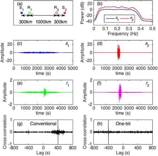
Synthetic tests of noise cross-correlation functions: (a) geometry, (b) source spectra, (c) source S1 time function, (d) source S2 time function, (e) receiver R1 record, (f) receiver R2 record, (g) normalized conventional cross-correlation function, and (h) normalized one-bit cross-correlation function. The records (e and f) were calculated using the Green's function given in eq. (8).
Cross-correlation functions between r1 and r2 are shown in Figs 1(g) and (h). The peak at negative lag (peak 1) corresponds to the signal from S1, while the peak at positive lag (peak 2) corresponds to the signal from S2. Note that both methods give accurate traveltimes (d12/c = 1000 km/2.5 km s−1 = 400 s). However, conventional cross-correlation indicates a dominant signal from S2, while one-bit cross-correlation indicates a dominant signal from S1. Specifically, the ratio between peak 2 and peak 1 is 5.8 in conventional cross-correlation function, which is close to the ratio between the arrival energy from the two sources |$\sum r_{22}^2/\sum r_{11}^2=6.4$|. In contrast, this ratio is much less than 1 in one-bit cross-correlation function as peak 2 is almost invisible. This is because conventional preprocessing conserves amplitude information and gives the correct dominant source direction, while one-bit preprocessing normalizes the received signal per time unit, thus over-emphasizing the long-duration weak signals from S1. Therefore, conventional preprocessing is a better choice for dominant source direction estimation.
4 METHOD COMPARISONS FOR A SELECTED STATION-PAIR
Different preprocessing methods on CI OBS observations affect DF microseism noise cross-correlation source direction estimation. The 2012 CI OBS array covers the Juan de Fuca Plate with inter-station separation of ∼70 km, see Fig. 2). Available stations in March 2012 include 13 shallow-water (depth < 200 m) stations, 9 intermediate-depth (200 m < depth < 2000 m) stations, and 31 deep-water (depth > 2000 m) stations. Twenty of the 53 available OBSs were designed to record along the continental shelf and slope of the Cascadia margin at less than 1000-m depth (Toomey et al.2014). However, we choose deep-water station-pair J31A and J30A because deep-water stations have higher SNR in cross-correlation functions because they do not include overhead ocean wave direct-pressure signals that decay exponentially with depth (described as hydrodynamic filtering), which could reduce SNR.
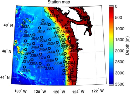
CI OBS stations map (March 2012). Colour represents seafloor depth. The three black contours are the coastline, the 200-m depth contour, and the 2000-m depth contour, from the thickest to the thinnest lines, respectively. Stations J06A, G30A and G03A are out of the plot region and are not shown in the map.
Observations at J31A (depth: 2657 m) and J30A (depth: 2824 m) during March 2012 were bandpass filtered from 0.115–0.145 Hz after correcting for the instrument response to displacement. This frequency band belongs to ocean-swell-generated longer-period double-frequency band in Bromirski et al. (2005), with further justification for choosing this band provided in Section 6. For clipping preprocessing, the records were divided into 31 single-day segments. The median of the 10 smallest RMS of these segments represents the noise level, denoted by RMSnoise. The clipping thresholds are obtained by multiplying RMSnoise by different factors (0.5, 5, 10, 20, higher thresholds give less clipping). Clipping with a sufficiently low threshold is used to minimize the effect of earthquake signals and other short-duration high-amplitude transients.
Although various preprocessing methods produce cross-correlation functions with peaks at similar lags (i.e. similar traveltimes), the ratios between the amplitudes of the two peaks at the positive and negative lag sides are significantly different, demonstrated in Fig. 3. Note that the negative lag peak corresponds to signals coming from west, with positive lag from the east. The ratio of the two peaks allows comparison of counter-propagating signals for one station-pair because the same background noise level and station separation would be used to calculate RSNR of both sides of the cross-correlation function. The conventional cross-correlation function has similar peak amplitudes on both sides, indicating no dominant source direction. Lowering clipping thresholds (increasing the amount of clipping) increases the ratio between the left and right peaks. One-bit and RAM preprocessing give similar cross-correlation functions as the strong factor of 0.5 clipping preprocessing, indicating a prominent dominant signal from west.
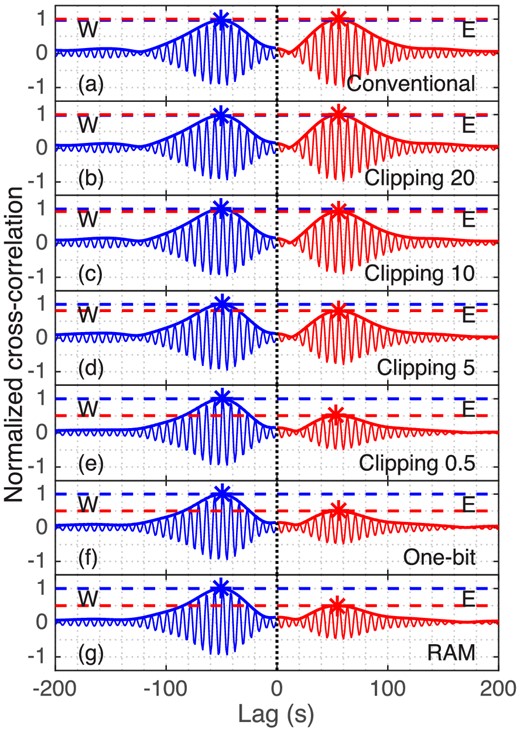
Comparison of cross-correlation functions (thin lines) and their envelopes (thick lines) between station-pair J30A and J31A for March 2012 in 0.115–0.145 Hz frequency band. Results are shown for preprocessing methods: (a) conventional; (b) clipping (threshold: 20 × RMSnoise); (c) clipping (threshold: 10 × RMSnoise); (d) clipping (threshold: 5 × RMSnoise); (e) clipping (threshold: 0.5 × RMSnoise); (f) one-bit; (g) running-absolute-mean (RAM). Signals coming from west (W, blue) and east (E, red) are indicated. Respective peaks and peak levels are represented by correspondingly coloured asterisks and coloured dashed lines.
Since preprocessing methods have such a significant influence on dominant source direction estimation, it is important to investigate changes in direction estimates over time for a particular event. We compare conventional preprocessing and one-bit preprocessing, which represents no-clipping (but earthquakes have been removed) and extreme clipping (RAM preprocessing with 5-point window length gives cross-correlation function peak levels similar to one-bit preprocessing). This shows differences between the cases at both ends of the clipping spectrum (Fig. 3). Amplitude and spectral characteristics are examined for the same station-pair (J30A and J31A) and frequency band (0.115–0.145 Hz) during March 4–7 observations. There was a small local earthquake on March 6, which was removed in conventional preprocessing (Figs 4b and d). It is almost invisible in 0.115–0.145 Hz. Similar results were obtained without removing this earthquake. Note that the first two days have higher power in the 0.115–0.145 Hz band, but have lower power in the 0.2–0.3 Hz band (Figs 4a and c), suggesting different source characteristics for the 0.115–0.145 Hz and 0.2–0.3 Hz microseism components. Consistent with the observations, wave model hindcast significant-wave-height Hs (WAVEWATCH-IIITM (Tolman 2009)) indicate ocean wave arrivals from strong distant storm in the first two days, followed by weak local storm events, and then quiet wave activity during the last two days (see movie in Supporting Information). Cross-correlation functions are given for the first two days (Figs 5a and b), last two days (Figs 5c and d), all four days (Figs 5e and f), and also whole March (Figs 5g and h).
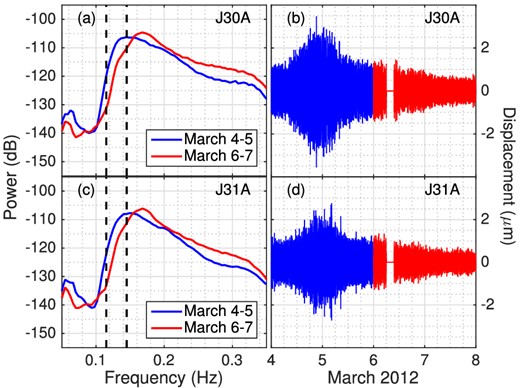
Spectra (left column) and 0.115–0.145-Hz-Butterworth-filtered waveforms (right column) of station J30A (top row) and J31A (bottom row) records in March 4–5 (blue) and March 6–7 (red). Spectra were calculated using Welch's method with 50 per cent overlapping 256-s data segments. The corner frequencies of the filter are indicated by the dashed lines. The small local earthquake on March 6 was removed, indicated by the gap.
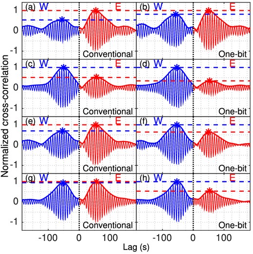
Conventional (left column) and one-bit (right column) cross-correlation functions (thin solid lines) and their envelopes (thick solid lines) for stations J30A and J31A with each row from top to bottom representing an observation time: (a, b) 4–5 March, (c, d) 6–7 March, (e, f) 4–7 March, and (g, h) 1–31 March. Signals coming from west (W, blue) and east (E, red), as well as the peaks (asterisks) and peak levels (dashed) are indicated.
Both preprocessing methods indicate a dominant signal from east during March 4–5 and a dominant signal from west during March 6–7. These results are consistent with coastal generation dominating when strong swell is present in shallow near-coastal water, with pelagic generation dominating otherwise.
The two methods indicate different dominant source directions for the combined time period, that is, March 4–7. Conventional cross-correlation indicates a dominant signal from east while one-bit cross-correlation indicates a dominant signal from the west. Additionally, the two methods also give different results for the whole month. Conventional cross-correlation indicates similar-strength signals from two directions while one-bit cross-correlation consistently indicates a dominant signal from the west.
Recall the synthetic test (Fig. 1), the difference between the source amplitude and duration characteristics could contribute to this distinction. Hindcast Hs spanning March 2012 show episodic distant storm waves and strong regionally-generated storm waves reaching the coastal region, likely producing relatively short-duration but high amplitude signals there. However, as these strong coastal-generated signals have short duration, persistent pelagic-generated signals could dominate most of the time, thus producing the differences between the two cross-correlation functions. One-bit normalization accentuates the pelagic-generated long-duration and but relatively weak signals, thus biasing the dominant source direction estimation. In order to examine the validity of this conjecture, we need to examine the source characteristics in coastal and pelagic areas.
5 SOURCE CHARACTERISTICS ANALYSIS
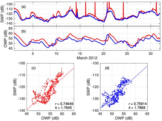
(a) Seismic wave power (SWP) of deep-water J31A (blue) and shallow-water J25A (red) records in 0.115–0.145 Hz frequency band and (b) spatial-linear-interpolated Ocean wave power (OWP) at J31A (blue) and J25A (red) in March 2012. SWP is characterized by hourly mean square of 0.115–0.145-Hz filtered seismogram, while OWP is calculated from eq. (9). Linear regressions of corresponding SWP and OWP (both in dB) for stations (c) J25A and (d) J31A are shown. SWP segments with earthquakes or other local transients are removed. OWP is temporal-interpolated to correspond to SWP segments.
As shown previously (Fig. 1), conventional cross-correlation is more sensitive to signal power while one-bit and RAM cross-correlation are more sensitive to signal duration. To investigate the power and duration characteristics of the sources, we calculate the ratio of the 5 per cent strongest segments’ power to the total power in 0.115–0.145 Hz band. Specifically, the record is 0.115–0.145-Hz bandpass filtered and then divided into consecutive 1-hour segments. Segments with earthquakes, missing data, or local transients (e.g. trawling, fish impacts) are removed. When a time segment is removed in one station record, the corresponding time segment is removed for all stations. The energy of each segment is represented by the mean of the squared record. The total energy of the 5 per cent strongest segments are calculated and divided by the total energy of all segments. This ratio reflects the percentage the strongest 5 per cent segments possess of the total energy. Thus, a larger ratio indicates more energy concentrated in the 5 per cent most energetic time. This ratio is significantly larger in coastal areas (especially in the northeast near Vancouver Island) than in pelagic areas, see Fig. 7(a), suggesting that shallow water could be the primary source area of short-duration high-amplitude signals. If this is the case, a lower west-to-east peak ratio in conventional cross-correlation functions than in one-bit cross-correlation functions is expected, since the eastern-generated short-duration strong signals would be underestimated by one-bit preprocessing. This is validated by Figs 5(g) and (h). The comparison on the entire array will be given in the next section.
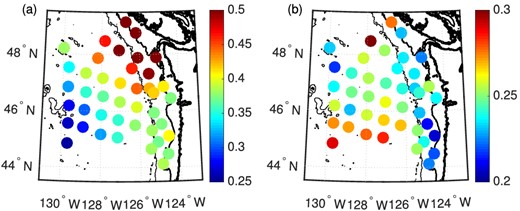
The energy ratio of the 5 per cent strongest spectral estimates to the total energy of March 2012. Frequency bands: (a) 0.115–0.145 Hz, (b) 0.2–0.3 Hz. The energy of each segment is represented by the mean of the squared record. The three black contours are coastlines, and the 200-m and 2000-m depth contours, thickest to the thinnest, respectively.
6 COMPARISON ON THE ENTIRE ARRAY
To show the advantage of using RSNR, we calculated both SNR and RSNR of the cross-correlation functions from conventional, one-bit and RAM preprocessing for the entire CI OBS array record, see Fig. 8. Stations J06A, G30A, and G03A are excluded for they are far from the main part of the array. SNR decreases with station separation roughly as |$1/\sqrt{d}$|, while RSNR is less related to station separation, suggesting that geometric spreading effect is minimized in RSNR. Thus, the dominant source direction will be better determined using RSNR.
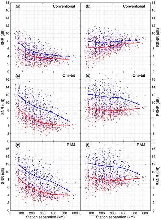
Station separation versus SNR (first column) or RSNR (second column) of the cross-correlation functions from conventional (first row), one-bit (second row) and RAM (third row) preprocessing of the CI OBS array records. SNR/RSNR for positive (signals from east, red dots) and negative (signals from west, blue dots) lags are indicated. Coloured solid lines are 100-km-window running average of the SNR/RSNR on the corresponding lag side. Frequency band: 0.115–0.145 Hz.
The two SNRs (one for each side, or equivalently, source direction), as well as the two RSNRs, of each cross-correlation function are much closer to each other with conventional preprocessing than with one-bit and RAM preprocessing, as shown in Fig. 8. This reflects the bias effect of one-bit and RAM preprocessing as demonstrated in Section 5.
To investigate the effect of preprocessing on identifying source direction, we first calculate RSNR for each station-pair in CI OBS array with conventional, one-bit and RAM preprocessing methods in 0.115–0.145 Hz band (first column in Fig. 9). The directions with highest RSNR values should be the dominant directions. Averages of RSNR values for 10° azimuth slices are presented for clarity. Only the outgoing wave (propagating to the other station) RSNRs are plotted, similar to Tian & Ritzwoller (2015). Note that here the arrows point to the source, while pointing away from the source in Tian & Ritzwoller (2015). Shallow-water station records have a higher background noise level than deep-water stations. Thus, on average, RSNR at shallow-water stations are lower than that at deep-water stations. Therefore, it's more reasonable to compare RSNR in different directions at one station than to compare RSNR between stations, especially between deep-water and shallow-water stations. Stations with RSNR values showing both pelagic and coastal directions (mostly inside the red frame in Fig. 9) are more informative. Conventional cross-correlation shows no notably dominant source direction while one-bit and RAM cross-correlations show a significantly dominant signal from the west, especially from the southwest. This is consistent with the source characteristic analysis that short-duration strong signals are mainly coastal-generated (sensitive to conventional preprocessing) while pelagic-generated signals are mostly weak but with long duration (sensitive to one-bit and RAM preprocessing) in the 0.115–0.145 Hz band. Thus the one-bit and RAM preprocessing artificially increase SNR only for long-duration relatively low-amplitude signals. This gives an erroneous source direction distribution.

Averaged 10° azimuth slices for RSNR of cross-correlation functions from conventional (first row), one-bit (second row) and RAM (third row) preprocessing for entire CI OBS array records in March 2012. Frequency band: 0.115–0.145 Hz (first column) and 0.2–0.3 Hz (second column). Cross-correlation functions shown are restricted to those with RSNR larger than 3 dB on both sides. 821, 833, 860, 856, 860 and 856 out of 861 station-pairs are chosen in (a) to (f), respectively. The contours are the same as in Fig. 7. The most important stations are enclosed by the red frame. Note that the first row have different colour scales.
For comparison, we also calculated the energy ratio of the strongest 5 per cent segments in the 0.2–0.3 Hz band, associated with the deep-water microseism peak (Bromirski et al.2013) (see second column in Fig. 7). The energy ratio is significantly smaller than that in the 0.115–0.145-Hz band, and has less variability with location. But the energy ratio is generally larger in pelagic areas (especially the southwest), which is opposite to the 0.115–0.145 Hz band (compare Figs 7a and b). The RSNR map for 0.2–0.3 Hz indicates a dominant signal from west for all preprocessing methods (second column in Fig. 9), suggesting pelagic-generated signals are both longer and stronger (in total energy sense) than coastal-generated signals in the 0.2–0.3 Hz band.
We chose the 0.115–0.145-Hz frequency band for several reasons: (1) The spectrum of J30A and J31A show that March 4–5 DF signal is stronger than March 6–7 DF signal only in this frequency band (Fig. 4), suggesting different source characteristics between 0.115–0.145-Hz microseism and higher-frequency (e.g. 0.2–0.3 Hz) DF microseism levels. (2) As was shown in this section, the conventional cross-correlation function is most different from both one-bit and RAM cross-correlation functions in this frequency band, that is, the source amplitude and duration effect is strongest in this frequency band. (3) Earthquake signals are easy to detect and remove in the DF band. Comparatively, there is more earthquake surface wave energy in the SF band. The SF band can also be contaminated by currents.
The 0.115–0.145-Hz DF band has some association with SF microseism band variability, with both dominated by excitation near the coast during a strong swell event. However, the possibility of SF band signals significantly affecting spectral levels in the DF band is minimal since the double-frequency criterion makes for good separation between SF and DF signals. Multiple sources with differing spectral characteristics at different locations could in some cases obscure source directions, but in general the DF signal levels are much stronger than primary microseism levels and so will dominate. Because bottom interaction decreases with increasing frequency (shorter wavelength), ocean waves at over 0.1 Hz produce progressively less SF energy in the DF band.
7 CONCLUSIONS
Preprocessing has a significant influence on the amplitudes of cross-correlation function peaks. One-bit and RAM preprocessing methods introduce a bias in dominant source direction estimation associated with signal duration. Because they do not conserve amplitude information, signals with long duration dominate the cross-correlation functions, even if their total energy is lower than strong signals with short duration from the opposite direction. Comparatively, because conventional preprocessing retains amplitude information, this method is more influenced by energy and less by duration, which makes it a better choice for dominant source direction determination.
The temporal variation of spectral characteristics across the deep-water CI array stations indicates that there are always DF microseisms in the deep ocean. In contrast, strong DF microseisms are generated near-shore when waves from a storm reach the shore, which occur intermittently on synoptic time scales. Therefore, ubiquitous pelagic-generated signals have a much longer duration time than relatively short-duration coastal-generated signals even though their total energy is similar. Cross-correlation functions from one-bit and RAM preprocessing show a significantly dominant pelagic source direction, while those from conventional preprocessing show no significantly dominant source direction. This is consistent with the source location characteristics.
REFERENCES
SUPPORTING INFORMATION
Additional Supporting Information may be found in the online version of this paper:
OceanWaveAnimation.avi
Please note: Oxford University Press is not responsible for the content or functionality of any supporting materials supplied by the authors. Any queries (other than missing material) should be directed to the corresponding author for the paper.
