


Abstract
Recently constructed models of crustal structure across Tibet based on surface wave data display a prominent mid-crustal low velocity zone (LVZ) but are vertically smooth in the crust. Using six months of broad-band seismic data recorded at 22 stations arrayed approximately linearly over a 440 km observation profile across northeastern Tibet (from the Songpan–Ganzi block, through the Qaidam block, into the Qilian block), we perform a Bayesian Monte Carlo joint inversion of receiver function data with surface wave dispersion to address whether crustal layering is needed to fit both data sets simultaneously. On some intervals a vertically smooth crust is consistent with both data sets, but across most of the observation profile two types of layering are required: a discrete LVZ or high velocity zone (HVZ) formed by two discontinuities in the middle crust and a doublet Moho formed by two discontinuities from 45–50 km to 60–65 km depth connected by a linear velocity gradient in the lowermost crust. The final model possesses (1) a mid-crustal LVZ that extends from the Songpan–Ganzi block through the Kunlun suture into the Qaidam block consistent with partial melt and ductile flow and (2) a mid-crustal HVZ bracketing the south Qilian suture coincident with ultrahigh pressure metamorphic rocks at the surface. (3) Additionally, the model possesses a doublet Moho extending from the Qaidam to the Qilian blocks which probably reflects increased mafic content with depth in the lowermost crust perhaps caused by a vertical gradient of ecologitization. (4) Crustal thickness is consistent with a step-Moho that jumps discontinuously by 6 km from 63.8 km (±1.8 km) south of 35° to 57.8 km (±1.4 km) north of this point coincident with the northern terminus of the mid-crustal LVZ. These results are presented as a guide to future joint inversions across a much larger region of Tibet.
1 INTRODUCTION
The expansion of seismic instrumentation in Tibet has led to the rapid emergence of velocity models of the Tibetan crust and upper mantle. The emplacement of broad-band seismometers, in particular, allows for the observation of surface waves based both on ambient noise (e.g. Yao et al.2006; Yang et al.2010; Zheng et al.2010; Zhou et al.2012; Karplus et al.2013) and earthquake data (e.g. Caldwell et al.2009; Feng et al.2011; Li et al.2013a,b; Zhang et al.2014). Studies based on surface waves provide information primarily about shear wave speeds in the crust and uppermost mantle beneath Tibet (e.g. Villasenor et al.2001; Yao et al.2008; Li et al.2009; Duret et al.2010; Huang et al.2010; Guo et al.2012; Yang et al.2012; Li et al.2013b; Xie et al.2013; Chen et al.2014). A positive attribute of surface wave studies is that information is spread homogeneously across much of Tibet, but at the price of relatively low resolution both laterally and vertically. The vertical resolution of models derived from surface waves presents a particular challenge, as surface waves do not image discontinuities in seismic velocities well. Receiver functions image internal interfaces better than surface waves and there have been several studies based on them across Tibet (e.g. Zhu & Helmberger 1998; Vergne et al.2002; Wittlinger et al.2004; Xu et al.2007; Shi et al.2009; Zhao et al.2011; Sun et al.2012; Yue et al.2012; Tian & Zhang 2013; Xu et al.2013b; Tian et al.2014; Zhang et al.2014). Receiver functions, however, only provide information near seismic stations and less powerfully constrain structures between interfaces than surface waves (e.g. Ammon et al.1990). The joint interpretation of receiver functions along with surface wave dispersion, however, provides information about vertical layering that surface waves alone may miss (e.g. Ozalabey et al.1997; Julia et al.2000; Bodin et al.2012; Shen et al.2013a). Using data from the USArray in the US, Shen et al. (2013a) present a method to invert receiver functions and surface wave dispersion jointly based on a Bayesian Monte Carlo method to produce a model of shear wave speeds (and other variables) along with uncertainties in the crust and uppermost mantle. Shen et al. (2013b,c) show that vertically smooth crustal models can fit both data sets acceptably except in several regions and, therefore, across most of the western and central US the introduction of layering within the crystalline crust is not required to fit the receiver function data used in their study.
The purpose of this paper is to address the same questions for Tibet with a particular focus on northeastern Tibet: (1) Can surface wave dispersion and receiver function data be fit simultaneously with vertically smooth models in the crystalline crust? (2) If not, then what is the nature of the discontinuities between the sediments and Moho that must be introduced to allow both data sets to be fit simultaneously? (3) Finally, what do the answers to these questions imply about the thickness and structure of the crust in northeastern Tibet?
In this study we use six months of data (late 2010 to mid-2011) from a linear array of 22 broad-band seismometers deployed in the Songpan–Ganzi block, the Qaidam block and the Qilian block of northeastern Tibet (Fig. 1, blue diamonds). We use these data to produce receiver functions (with uncertainties) at 23 evenly spaced geographical locations spanning a distance of 440 km along the ‘observation profile’. Using the method of Shen et al. (2013a), we jointly invert these receiver functions along with Rayleigh wave phase speed data taken from the study of Xie et al. (2013) to produce shear velocity models (with uncertainties) of the crust and uppermost mantle beneath the observation profile. We produce two models, one that varies smoothly vertically in the crystalline crust (Model 1) and another one (Model 2) that allows for crustal discontinuities that are adapted to the receiver functions. In contrast to the US (Shen et al.2013b,c), we present evidence here that across most of the observation profile crystalline crustal discontinuities and/or a doublet Moho are needed to fit the receiver functions.
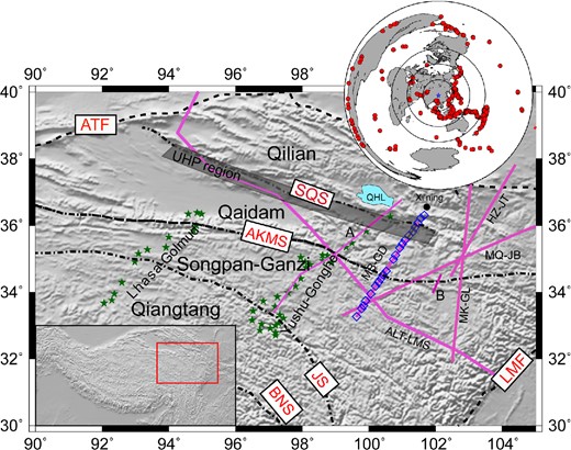
The inset map presents locations of the distribution of teleseismic earthquakes used in this study. Blue diamonds are the locations broad-band seismometers used in this study; green stars are earlier seismic stations from the Lhasa-Golmud and Yushu-Gonghe profiles. Deep seismic sounding profiles and seismic reflection profiles include the following: HZ-JT: Hezuo–Jingtai profile (Zhang et al.2013); MB-GD: Moba-Guide profile (Zhang et al.2011a); ALT-LMS: Altyn Tagh–Longmenshan profile (Wang et al.2013); MK-GL: Markang–Gulang profile (Zhang et al.2008); MQ-JB: Maqin–Jingbian profile (Liu et al.2006); A: Galvé et al.(2002); B: Wang et al. (2011). Geological features include: ATF: Altyn Tagh fault; BNS: Bangong–Nujiang suture; LMF: Longmenshan fault; JS: Jinsha suture, AKMS: Animaqing–Kunlun–Muztagh suture (or Kunlun fault), SQS: south Qilian suture and the Songpan–Ganzi, Qaidam block and Qilian blocks are identified. The region with ultrahigh pressure (UHP) metamorphism is identified by the grey rectangle (Yang et al.2002).
The crust in northeastern Tibet has already been the subject of studies based on seismic reflection and refraction profiling (see Fig. 1) as well as receiver functions (e.g. Vergne et al.2002; Shi et al.2009; Zhao et al.2011; Yue et al.2012; Tian & Zhang 2013; Xu et al.2013b; Tian et al.2014). These studies have observed significant variations in crustal structure (e.g. Karplus et al.2011; Mechie et al.2012) and thickness, including in some cases stepwise thickening of Moho (e.g. Zhu & Helmberger 1998; Vergne et al.2002; Wittlinger et al.2004; Jiang et al.2006). Understanding such variations is critical to test conflicting hypotheses related to the formation and evolution of the Tibetan plateau (e.g. Molnar et al.1993; Tapponnier et al.2001). Northeastern Tibet also is the site of choice to study remote effects of the India-Asia collision (Metivier et al.1998; Meyer et al.1998; Chen et al.1999; Pares et al.2003). In addition, the region contains the Caledonian orogeny and petrological and isotopic data point to high pressure and ultrahigh pressure (UH/UHP) metamorphism (Liu et al.2003; Luo et al.2012), which is inferred from the presence of eclogite and garnet peridotite as well as coesite-bearing gneiss in the north Qaidam (Song 1996; Yang et al.2002; Song et al.2006). Such metamorphism may have been caused by the burial and exhumation of the metamorphic rocks in the uppermost mantle along a Palaeozoic subduction zone (e.g. Yin et al.2007).
We are, nevertheless, unaware of previous studies based on the joint inversion of surface wave data and receiver function across northeastern Tibet. Other researchers have performed such joint inversions elsewhere in Tibet, notably in southeast Tibet or southwest China (e.g. Li et al.2008; Sun et al.2014; Wang et al.2014; Bao et al.2015) and the Lhasa terrane (e.g. Xu et al.2013a). Thus, the models produced in this study both may guide future joint inversions at large scales across Tibet and also provide new information about the structure and thickness of the crust in northeastern Tibet.
In Section 2, we discuss the receiver function and surface wave phase speed data sets that we use in the joint inversion. The hypothesis test to determine if crystalline crustal layering is needed and its characteristics are presented in Section 3, in which we contrast model characteristics and data fit with and without intra-crustal layering. In Section 4, we discuss the implications of the final crustal velocity model (Model 2) in terms of mid-crustal partial melt in the Songpan–Ganzi block and its potential intrusion into the Qaidam block, the coincidence of a mid-crustal high velocity zone (HVZ) with HP/UHP rocks in the Qaidam block, the nature and location of the Moho doublets and the step-Moho along the observation profile, and finally compare our estimates of crustal thickness with earlier studies in the region.
2 DATA AND METHODOLOGY
Between November 2010 and June 2011, a passive seismic experiment was carried out by the Institute of Geology and Geophysics, Chinese Academy of Sciences, from the Songpan–Ganzi block to the Qilian block (Fig. 1). Twenty-two broad-band seismographs (Reftek-72A data loggers and Guralp CMG3-ESP sensors with 50 Hz–30 s bandwidth; represented by the blue diamonds in Fig. 1) were deployed at intervals of about 20 km. The profile covers the northeastern margin of the Tibetan plateau. The northwest–southeast trending Animaqing–Kunlun–Muztagh suture (Kunlun fault) and the south Qilian suture divide the profile into three principal geological units: the Songpan–Ganzi block, the Qaidam block and the Qilian block.
2.1 Receiver functions
2.1.1 Sensor orientation
Misorientation of sensors will cause amplitude errors in receiver functions (Niu & Li 2011). Before computing the receiver functions, we attempt to determine station orientation using P-wave particle motions (e.g. Niu & Li 2011). A misorientation less than 7° in azimuth is not expected to affect receiver functions or surface wave polarizations significantly (Niu & Li 2011). We found that only one of the 22 stations exhibited a misorientation azimuth larger than 7°, and corrected the orientation for this station.
2.1.2 Calculation of receiver functions
2.1.3 Quality control
Figure 2 presents an example of the result of the quality control process for station DKL21 whose location is identified in Fig. 3. The original receiver functions from 360 earthquakes are presented in Fig. 2(a) separated by azimuth. Most receiver functions are from earthquakes at azimuths between about 40° and 200°, which are from the northeast to the south of the study region. Substantial disagreement among the receiver functions is apparent in Fig. 2(a). After quality control Steps 1 and 2, the number of receiver functions reduces to 149 as shown in Fig. 2(b). The 111 azimuthally smooth receiver functions that emerge from the harmonic analysis of Step 3 are shown in Fig. 2(c). After the quality control process is complete, we retain a total of 1145 receiver functions for the 22 stations along the profile.
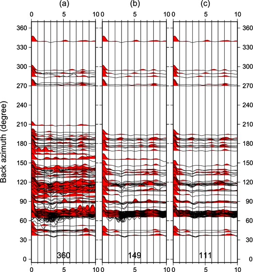
Example of the quality control process for receiver functions (RFs) at station DKL21. (a) The full set of 360 observed RFs are plotted versus backazimuth. (b) The 149 residual RFs after quality control steps 1 and 2. (c) The final 111 RFs after harmonic stripping, quality control step 3, in which only RFs that vary smoothly with azimuth are retained.
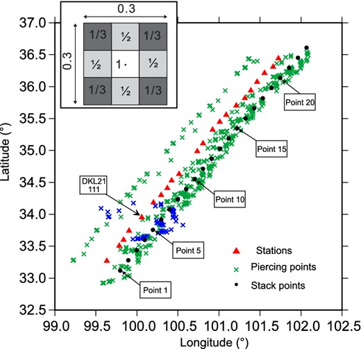
Red triangles mark the locations of the 22 stations along the observation profile and green crosses show Moho piercing (or conversion) points (red crosses) of the incident P waves. Blue crosses are Moho piercing points for station DKL21 (identified). The black dots indicate the stacking locations, which are separated by 20 km and numbered 1–23 (shown). The inset box contains the weights used to stack the receiver functions.
2.1.4 Receiver function CMCP stacks
Shen et al. (2013a,b) advocated for the use of the function A0(t) from eq. (2) as representative of the azimuthally independent structure beneath the station. However, Fig. 2 shows that the distribution of earthquakes in our study produces receiver functions that lie primarily in the azimuthal range from 40° to 200°, so A0(t) may be biased by azimuthally dependent structure near the station. Figure 3 further illustrates this point by presenting the locations of the Moho piercing points of P waves (or P to S conversion points) retained after quality control. Moho piercing points are computed by ray tracing from each earthquake through a model with P velocities from IASP91 (Kennett & Engdahl 1991) but with crustal thickness from Xu et al. (2014). The piercing points are predominantly to the east and southeast of the stations at which the receiver functions are observed and are characteristic of structures there rather than near the stations. For this reason, we use harmonic stripping only for quality control and not to produce the stacked receiver functions at the stations. Rather, we stack receiver functions along the observation profile at a set of 23 stacking locations lying at 20 km intervals (Fig. 3, black dots, numbered 1–23). We stacked (i.e. averaged) the receiver functions with Moho piercing points lying within 0.15° of each stacking location. We refer to this as the common Moho conversion point (CMCP) stacking method, which is somewhat similar to the CCP (common conversion point) stacking method (e.g. Dueker & Sheehan 1998). The weights used in stacking are shown in the inset panel in Fig. 3 showing nine square sub-boxes with sides of 0.1°. In each sub-box, we average all receiver functions with equal weight producing what we call a sub-box receiver function. Then the sub-box receiver functions are stacked (averaged) according to the weights presented in the inset panel where the central sub-box lies on the stacking location. The stacking locations together form what we call the ‘observation profile’.
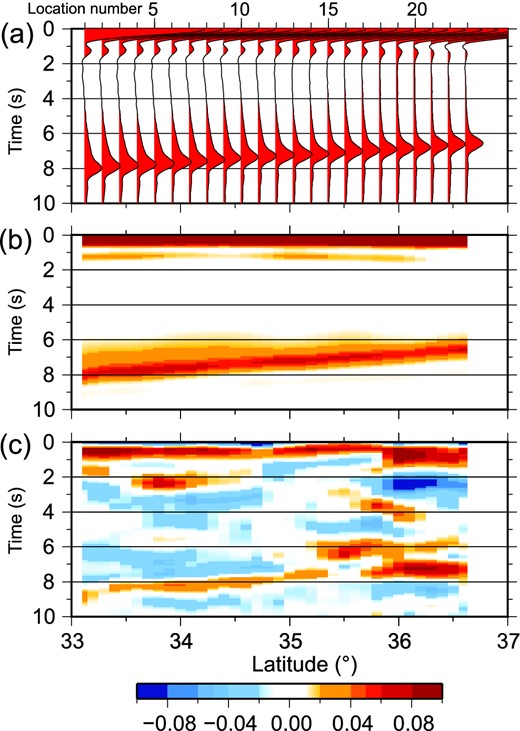
Figures 4(b) and (c) present the stacked receiver functions along the observation profile with locations identified by the location numbers 1–23. Figure 4(b) shows the stacked receiver function waveforms themselves and Fig. 4(c) shows the same information but with amplitude-dependent colour shading. The P and P-to-S converted phases from the Moho can be seen clearly along the profile. The delay time between the P and P-to-S converted phases from the Songpan–Ganzi block (SB) to the Qilian block (QL) varies from about 7 to 8 s. This delay time reduces northward along the stacking profile and becomes more complicated, showing a double peak at most locations north of stacking location 12. Additional complexities in the receiver functions also appear in Fig. 4, which are discussed later in the paper.

(a) The elevation along the observation profile. (b) Moho conversion point (MCP) stacked receiver functions are illustrated with red waveforms as a function of the stacking location number. (c) Smoothed colour-coded image of the receiver functions.
We also estimate uncertainties for each receiver function along the profile. First, we compute the standard deviation at each time among the receiver functions in each stacking sub-box. We then take the weighted average of these standard deviations to compute the uncertainty of the stacked receiver function, using the weights given in the inset panel of Fig. 3. An example of these one standard deviation uncertainties can be seen for location 13 as the grey shaded envelope in Fig. 5(a).
2.2 Rayleigh wave phase velocity
Xie et al. (2013) mapped phase velocities across eastern Tibet and surrounding regions for Rayleigh (8–65 s) and Love (8–44 s) waves using ambient noise tomography based on data from the Program for Array Seismic Studies of the Continental Lithosphere (PASSCAL) and the Chinese Earthquake Array (CEArray). In that study, uncertainties of the surface wave phase speeds were also obtained by performing eikonal tomography (Lin et al.2009). We interpolate the Rayleigh wave phase speed and uncertainty curves beneath the stacking points, an example of which is shown in Fig. 5(b) for location 13. Rayleigh wave phase speeds increase from about 3.1 km s−1 at 8 s period to about 3.85 km s−1 at 65 s period, and the uncertainty also increases with the period. Other example Rayleigh wave phase speed curves are presented later in the paper.
2.3 Joint inversion of receiver functions and surface wave dispersion
Internal interfaces such as sedimentary basement and Moho are difficult to resolve based on the inversion of surface wave data alone. While surface wave dispersion constrains well the vertically averaged velocity profile, it only weakly constrains velocity interfaces and strong velocity gradients. Receiver functions have complementary strengths to surface wave data (e.g. Ozalaybey et al.1997; Julia et al.2000; Du et al.2002; Li et al.2008) and the joint inversion of surface wave dispersion with receiver functions may be more reliable than structures derived exclusively on either data set alone (e.g. Julia et al.2003, 2005; Chang & Baag 2005; Shen et al.2013a,b). Shen et al. (2013a) developed a non-linear Bayesian Monte-Carlo algorithm to estimate a Vs model by jointly interpreting Rayleigh wave dispersion and receiver functions as well as associated uncertainties. We apply this method here. We apply stacked receiver functions in the 0–11 s time band and Rayleigh wave phase speeds between 8 and 65 s period at 20 km intervals along the observation profile. This time band and period range provides information about the top 80 km of the crust and uppermost mantle. In the models presented here, both the inversion of surface wave data performed by Xie et al. (2013) and the joint inversions of surface wave data and receiver functions presented for the first time here, we apply a Vp/Vs ratio of 1.75 in both the crust and uppermost mantle. We choose to fix this ratio primarily for consistency with the starting model (Xie et al.2013). There is no doubt, however, that Vp/Vs varies with depth and along our observation profile. The Vp/Vs ratio trades off with crustal thickness and structures within the crust and, therefore, the depth to Moho and the amplitude and depth of structural features in the crust will depend on this choice.
3 CRUSTAL STRUCTURE ALONG THE PROFILE
3.1 Smooth starting model from surface waves alone
We start with the model of Xie et al. (2013), which is determined from Rayleigh and Love wave phase speed measurements alone determined from ambient noise tomography. (For the background to this study see: Shapiro et al.2004; Bensen et al.2007; Lin et al.2008, 2009; Zheng et al.2008; Yang et al.2010, 2012; Ritzwoller et al.2011; Zheng et al.2011; Zhou et al.2012). The model is composed of three layers stacked vertically with variable thicknesses but the crystalline crust is vertically smooth. The top layer is the sediments, which are isotropic (Vs = Vsv = Vsh) with constant velocity vertically. The middle layer is the crystalline crust, which is radially anisotropic (Vsv ≠ Vsh). Each of Vsv and Vsh is given by five B-splines in the crystalline crust. The bottom layer is the radially anisotropic uppermost mantle in which Vsv is given by five B-splines and the difference between Vsh and Vsv is taken from an earlier model of the region (Shapiro & Ritzwoller 2002; Shapiro et al.2004). Sedimentary thickness and Moho depth were free variables in the inversion for this model, which applied several constraints including vertical crustal smoothness and positive jumps at the base of the sediments and crust. For the purposes here, we only use the Vsv part of the model at all depths and set the model to be isotropic (Vs = Vsv = Vsh) because we only invert Rayleigh waves and receiver functions. The Vp/Vs ratio both in the crust and mantle is set to 1.75.
A plot of Vsv as a function of depth along the observing profile is presented in Fig. 6(a). In this model the crust thins slowly and continuously to the north from about 61.5 km in the Songpan–Ganzi block to 51.5 km in the Qilian block. More prominently, in the Songpan–Ganzi block mid-crustal Vsv is very slow, much slower than in the Qilian block. Hacker et al. (2014) argue that such slow shear velocities must be caused by partial melt in the middle crust.
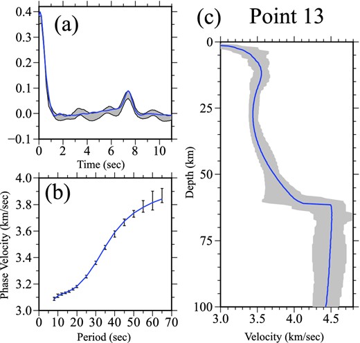
Example of data and inversion result at location number 13. (a) The observed receiver function (with uncertainty) is presented as the grey envelope. (b) The observed Rayleigh wave phase speed curve (with uncertainties) is plotted with one standard deviation error bars. (c) The full (grey) envelope of accepted models in the posterior distribution from the joint inversion of the receiver function and dispersion data with a smoothly varying crystalline crust (i.e. Model 1). The blue lines in (a) and (b) show the predicted data from the best-fitting model and the blue line in (c) presents the mean of the posterior distribution at each depth.
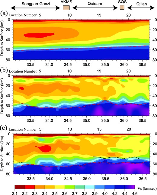
The three models discussed here, all are Vsv (km s−1). (a) The starting model from Xie et al. (2013) constructed with Rayleigh wave dispersion data alone. (b) Model 1, which results from the joint inversion of receiver functions and Rayleigh wave dispersion without discontinuities in the crystalline crust. (c) Model 2, which results from the joint inversion of receiver functions and Rayleigh wave dispersion with discontinuities in the crystalline crust at the locations specified in Table 1.
(a) The computed receiver functions (RFs, red lines) from the starting model of Xie et al. (2013). (b) A smoothed colour-coded image of the computed RFs. (c) The difference between computed RFs and observed RFs.
3.2 Joint inversion of surface waves and receiver functions with a vertically smooth crystalline crust: Model 1
To begin to model the complexities in crustal structure implied by the receiver functions and inferred in Section 3.1, we first perform a joint inversion of the Rayleigh wave dispersion data and the receiver functions at each location along the profile but continue with the constraint that the model is vertically smooth in the crystalline crust. We refer to this model as having resulted from the vertically smooth joint inversion or as Model 1. Data such as those shown in Figs 5(a) and (b) are inverted jointly using the method described by Shen et al. (2013a,b). The starting model is the model of Xie et al. (2013) and we adopt the parametrization of this model with three modifications: (1) the model is isotropic at all depths (there is no radial anisotropy) such that Vs = Vsv, (2) we use seven B-splines for Vsv in the crust rather than five and (3) we represent sedimentary velocities as a linear monotonically increasing function of depth rather than a constant. Importantly, as crystalline crustal structure is represented with B-splines, although larger in number than in the model of Xie et al. in this inversion the crystalline crust still is constrained to be smooth vertically. In Section 3.3, this constraint is broken in order to introduce internal crustal interfaces that appear to be needed in order to fit the receiver function data.
We perform the inversion with a Bayesian Monte Carlo method aimed to fit the Rayleigh wave dispersion and receiver functions jointly and equally well at each location along the observation profile. Uncertainty estimates in each type of data weight the relative influence of each data type in the likelihood function (i.e. misfit) and the inversion results in a posterior distribution of models that fit the data acceptably at each depth. Figure 5(c) shows the results of the inversion at Point 13 along the observation profile, presented with a grey corridor that represents the full width of the posterior distribution at each depth. The blue line is the mean of the posterior distribution at each depth.
The mean value of the posterior distribution for Vsv at each depth along the observation profile is presented in Fig. 6(b). Compared with the starting model from Xie et al. (2013) determined from surface wave data alone in Fig. 6(a), vertical variations in Model from 1 are sharper; for example, the mid-crustal velocities in the Songpan–Ganzi block are confined to a narrower depth range, and are faster and overlain by a thin veneer of higher velocities at about 10 km depth. There are higher velocities in the lowermost crust (50–60 km) bracketing the Kunlun fault and the mid-crustal velocities in the Qilian block are generally faster although very low velocities appear in the lowermost crust south of the south Qilian suture.
Figures 8(a) and (b) present the synthetic receiver functions computed from Model 1. A comparison, in particular, between the observed receiver functions in Fig. 4(c) and the synthetics in Fig. 8(b) illustrates the improvement in fit via the introduction of vertically smooth internal crustal structures that nevertheless produce receiver function arrivals between the direct P arrival and the P-to-S conversion. Figure 8(c) quantifies this comparison by presenting the difference between the observed and synthetic receiver functions. Contrasting Fig. 8(c) with Fig. 7(c) shows that the fit to the receiver functions is greatly improved compared with the model of Xie et al. even though the model remains vertically smooth in the crust. The overall χ2, defined by eq. (4), is 1.4, which represents a 72 per cent reduction in the variance relative to the starting model. Therefore, the introduction of receiver functions in the joint inversion is advisable even when retaining a vertically smooth model.
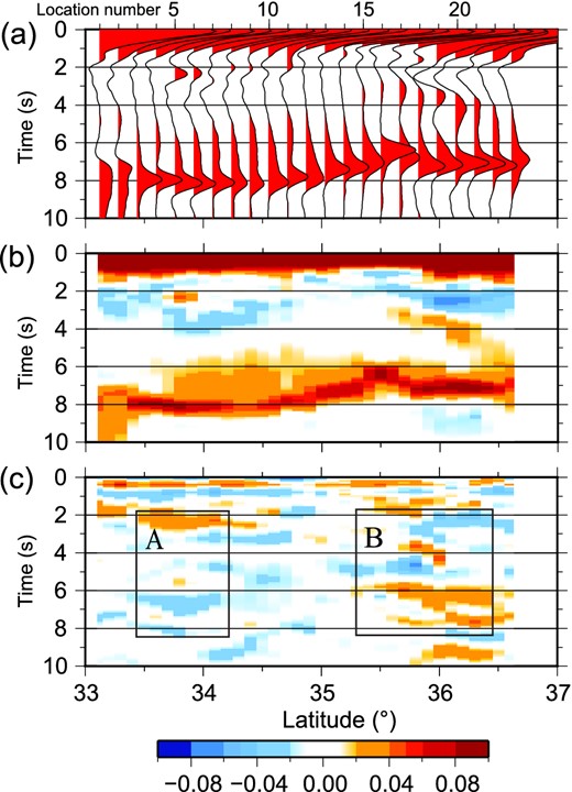
Similar Fig. 7, but here receiver functions are computing using Model 1, which results from the joint inversion of receiver functions and Rayleigh wave dispersion without discontinuities in the crystalline crust. The boxes denoted (A) and (B) identify areas in which we particularly seek to improve the fit to the receiver functions.
Nevertheless, there remain considerable differences between the observed and synthetic receiver functions, particularly in the boxes marked (A) and (B) in Fig. 8(c). This can be seen more clearly in Fig. 9, which presents vertical profiles beneath Point 6 (box A) and Point 18 (box B) from Model 1 as the red lines in Figs 9(a) and (d), respectively. (Blue lines and the corridor of accepted models are discussed later, in Section 3.3.) Figures 9(a) and (d) (red lines) illustrate how the receiver functions at these two points are misfit by Model 1. The misfit in the receiver function near Point 6 is somewhat subtle, but at Point 18 the double peak between 6 and 8 s cannot be fit with this model and neither can the swings in the receiver function between 3 and 5 s.
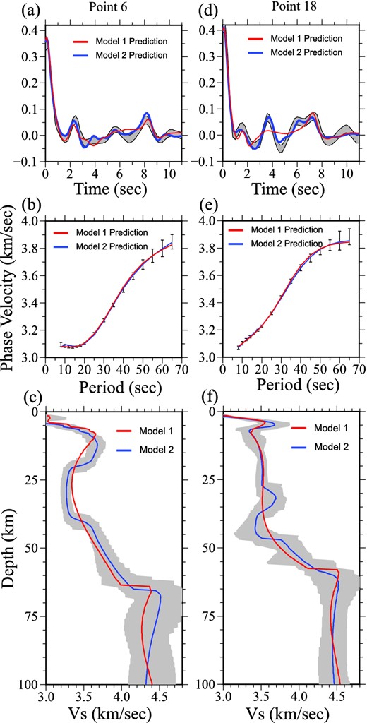
Similar to Fig. 5 in which example data and fits to receiver functions are presented for two sample points: 6 (left column) and 18 (right column), which lie in the boxes marked (A) and (B) in Fig. 8. Fits to the observed receiver functions and Rayleigh wave phase velocities by both Models 1 and 2 are presented as red and blue lines, respectively, in (a), (b), (d) and (e). Red and blue lines in (c) and (f) represent the best-fitting model of Model 1 (red) and Model 2 (blue). The full envelope of accepted models in the inversion with crustal discontinuities (Model 2) is shown in (c) and (f).
For these reasons, it is necessary to move beyond vertically smooth crystalline crustal models in order to fit the receiver function data in Tibet at least in some (perhaps most) locations. Interfaces within the crust are needed, therefore, to fit the receiver function data in detail. This is a different conclusion than drawn by Shen et al. (2013b,c) for the western and central US, where vertically smooth crystalline crustal models were found to suffice to fit surface wave dispersion and receiver function data jointly except in isolated areas across this region. Of course, the crust is much thinner in the US than in our region of study.
3.3 Joint inversion of surface waves and receiver functions with a layered crystalline crust: Model 2
To move beyond the vertically smooth crystalline crustal model from the joint inversion presented in Section 3.2 (Figs 6(b) and 8), we introduce different mid-crustal discontinuities in Regions 1, 2 and 3, which are identified in Table 1.
Locations and types of crustal discontinuities.
| Region number | Structures introduced | Location numbers | Latitude range |
|---|---|---|---|
| 1 | Slow mid-crustal layer | 5–7 | 33.6°–34.2° |
| 2 | Moho doublet + fast mid-crustal layer | 17–20 | 35.6°–36.2° |
| 3 | Moho doublet | 1–2 | 33.1°–33.3° |
| 14–16 | 35.1°–35.6° | ||
| 21–22 | 36.2°–36.5° |
Region 1 encompasses latitudes between about 33.6° and 34.2°, locations numbered 5–7, which lie in the northern part of the Songpan–Ganzi block to the Kunlun fault. In this region we introduce two mid-crustal discontinuities to the starting model, one at 20 km depth and one at 40 km depth and allow a constant velocity perturbation between them. The depths of these discontinuities and the amplitude of the perturbation are introduced as free variables in the inversion. The result at Point 6, which is contained in Region 1, is shown in Fig. 9(c). The grey envelope denotes the full width of the posterior distribution, the blue line marks the mean of the posterior distribution at each depth and the red line is the mean of the posterior distribution of Model 1 (Section 3.2). The introduction of these three degrees of freedom acts to restrict the depth extent of the low velocity zone (LVZ) in the central crust, increase the shear wave speed across most of the lower crust and reduce crustal thickness relative to Model 1. The result is a considerably better fit to the receiver function (blue line in Fig. 9a), particularly the P-to-S Moho conversion phase that appears near 8 s.
Region 2 lies between latitudes of about 35.6° and 36.2°, locations numbered 17–20, which is the northern part of the Qaidam block to the southern Qilian block, encompassing the southern Qilian suture. In this region the receiver functions are more complicated than elsewhere along the profile, and we introduce six degrees of freedom to the starting model. First, we introduce two mid-crustal discontinuities at 30 km and 40 km depth and allow a constant velocity perturbation between them. These three degrees of freedom allow for a HVZ in the central crust to develop. Second, we also allow for a ‘doublet Moho’ by introducing three more degrees of freedom to produce a linear velocity gradient in the lowermost crust (or uppermost mantle) with variable depth and upper and lower shear velocities. The result at Point 18, which is contained in Region 2, is shown in Fig. 9(f). An HVZ is introduced in the middle crust between depths of about 30–40 km and there are two prominent discontinuities that compose the doublet Moho, one near 45 km and another nearer to 60 km depth with a linear velocity gradient between these depths. The result is a much better fit to the receiver function (blue line in Fig. 9d), including the double P-to-S Moho conversion phase that appears between 6 and 8 s, the positive swing near 3.5 s and the negative swings near 2.5 and 4.5 s.
Finally, Region 3 comprises a discontinuous set of locations numbered 1–2, 14–16 and 21–22. In these locations we allow for a doublet Moho. Two of these ranges of points bracket Region 2, which also contains a doublet Moho, and the third occurs at the southern end of the observation profile. The locations with a doublet Moho are made clearer later in Fig. 11, discussed later in the paper.

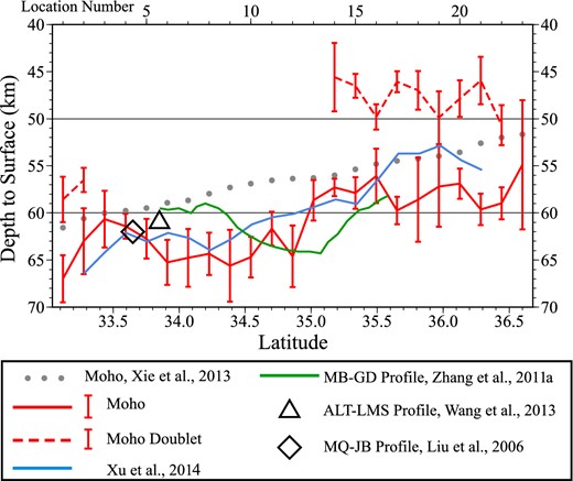
Our estimates of crustal thickness are presented with red error bars (1 standard deviation). Where we infer a doublet Moho the lower interface is interpreted as Moho (red solid line) and the upper interface is identified with the red dashed line. Crustal thickness from Xie et al. (2013) is presented with grey dots, from the receiver function study of Xu et al. (2014) is presented with the blue line and from the deep seismic sounding study of Zhang et al. (2011a) with the green line. The symbols (diamond and triangle) mark crustal thickness estimates from crossing lines (Liu et al.2006; Wang et al.2013).
The receiver functions in Figs 10(a) and (b) computed with the introduced mid-crustal discontinuities of Model 2 fit the observed receiver functions in Figs 4(b) and (c) much better than either the starting model or Model 1, particularly in Box B. The total reduced χ2 (eq. 3) is 0.9, which is a 82 per cent variance reduction relative to the starting model and a 36 per cent variance reduction relative to Model 1. The residual is small across most of the profile with the principal exception at times greater than about 7 s near the south Qilian suture (Box B), which we believe may be due to further layering in the uppermost mantle near the Qilian block.
Model 2, the model from the joint inversion with the layers introduced in the crystalline crust, is shown in Fig. 6(c). The LVZ near 34° latitude in the Songpan–Ganzi block has been accentuated further by lowering the minimum velocities and the uppermost and lowermost crust has correspondingly been made faster. More substantially, the model between 35.5° and 36.2° latitude, bracketing the south Qilian suture, now has an HVZ introduced near a depth of 35 km with a doublet Moho (as shown).
In summary, the surface wave dispersion data and receiver functions can be fit with at smooth crustal model across part of the observation profile, principally between location numbers 8–14 in the middle of the observation profile, but not in Regions 1–3 (Table 1). In these regions, crustal discontinuities must be introduced to fit the receiver functions. In Region 1, this produces a vertically narrower LVZ with a lower shear wave speed minimum. Region 2 is more complicated, requiring an HVZ in the middle crust. Beneath Regions 2 and 3 a doublet Moho at depths of about 50–60 km provides a significant improvement in fit to the receiver functions.
4 DISCUSSION
4.1 Mid-crustal LVZ in the Songpan–Ganzi block: evidence for partial melt
Crustal LVZs have been identified across Tibet by a number of studies (e.g. Kind et al.1996; Cotte et al.1999; Rapine et al.2003; Shapiro et al.2004; Xu et al.2007; Caldwell et al.2009; Guo et al.2009; Li et al.2009; Yao et al.2008, 2010; Acton et al.2010; Jiang et al.2011). Yang et al. (2012) summarize evidence from surface waves for a mid-crustal LVZ across much of Tibet. Such evidence generally supports the internal deformation model of Tibetan evolution where the medium is treated as a non-rigid continuum (e.g. England & Houseman 1986; England & Molnar 1997) and may particularly favour ductile ‘channel’ flow in the middle and/or lower crust (e.g. Bird 1991; Clark & Royden 2000; Searle et al.2011). Based on the more recent model of crustal shear velocities of Xie et al. (2013), our starting model presented along the observation profile in Fig. 6(a), Hacker et al. (2014) argue that the low mid-crustal shear velocities across Tibet are indicative of partial melt. In the region of study, if we identify the LVZ as shear wave speeds (Vsv) below 3.4 km s−1 in the middle crust, then the LVZ extends from the Songpan–Ganzi block through the Kunlun fault into the Qaidam block as far north as 34.9° (Fig. 6a). In this region, the Vp/Vs ratio was identified by Xu et al. (2014) to be greater than 1.75. As elsewhere in Tibet, block or terrane boundaries do not appear to obstruct crustal LVZs in the middle to lower crust (e.g. Yang et al.2012; Jiang et al.2014). Here, we ask the question whether the introduction of receiver functions in Region 1 (identified in Table 1) in the inversion increases or decreases the likelihood of partial melt in the middle crust.
First, in the results of the joint inversion of Rayleigh wave dispersion and receiver functions with an imposed crustal vertical smoothness constraint (Model 1, Fig. 6b), the shear velocities in the middle crust actually rise compared to the starting model constructed with surface wave data alone (Fig. 6a). This somewhat reduces the likelihood of partial melt in the middle crust. This rise occurs because the attempt to fit the receiver functions with a vertically smooth crystalline crust increases crustal thickness, which reduces predicted Rayleigh wave speeds in the period band sensitive to the middle and lower crust and the increased mid-crustal shear wave speeds compensate. Minimum Vsv speeds in the middle crust beneath the Songpan–Ganzi block in Model 1 mostly lie between 3.3 and 3.4 km s−1 but are somewhat lower in the starting model (Fig. 6a).
However, when two mid-crustal discontinuities are introduced in the joint inversion (Model 2, Fig. 6c) in order to improve the fit to the receiver function data, then the LVZ is accentuated in the middle crust beneath the Songpan–Ganzi block. In particular, the transitions to the LVZ from above and below are sharper, the LVZ is confined to a narrower depth range (20–40 km as opposed to 15–45 km) and the minimum shear wave speeds are lowered by about 0.1 km s−1, which makes partial melt more somewhat more likely than in the model of Xie et al. (2013). Moreover, by introducing the mid-crustal discontinuities to improve the fit to the receiver functions, sharp transitions are obtained within and outside of the mid-crustal LVZ beneath the northern Tibet. As proposed by Hacker et al. (2014), the melt produced in the middle and lower crust may have accumulated atop the melted zone at 20–30 km beneath the surface of the high plateau. The sharp reduction in Vs we observe above the LVZ at a depth of ∼20 km may be due to such a mechanism, serving as more evidence in favour of partial melt in addition to the minimum shear wave speeds.
Consequently, improving the fit to receiver functions by introducing internal crustal discontinuities modifies the shape and nature of LVZ beneath northern Tibet but does not reduce the likelihood of mid-crustal partial melt. Rather, it results in a slight increase in the likelihood of mid-crustal partial melt.
4.2 Mid-crustal HVZ in the Qilian block: coincident with HP/UHP metamorphism
The Qilian Caledonian orogenic belt is believed to be the product of the convergence and collision between the north China Craton with the Qilian and Qaidam terranes during the Early Palaeozoic Era (Yang et al.2001). UHP metamorphic rock are found along and near the south Qilian suture and several geological and tectonic models have been proposed to explain the origin of these rocks (Wang & Chen 1987; Yang et al.1994, 2002; Song et al.2006, 2009; Yin et al.2007; Zhang et al.2009). The crust near the south Qilian suture is known to be geophysically complicated, possessing highly variable Vp/Vs ratios (e.g. Xu et al.2014), high and variable residual Bouguer gravity anomalies (EGM2008; Pavlis et al.2012) and complicated receiver functions (e.g. Vergne et al.2002; Xu et al.2014). Our crustal model adds to this picture of crustal complexity by introducing a prominent high velocity anomaly at a depth of about 35 km that brackets the south Qilian suture (latitudes from 35.6° to 36.2°) directly below and adjacent to surface outcrops of UHP metamorphic rocks. We believe that the most likely interpretation is that this anomaly results from compositional heterogeneity, presumably of relatively enriched mafic rocks. Whether and how this anomalous structure relates to the UHP metamorphic rocks of the areas remains an area for further investigation.
4.3 The ‘Doublet Moho’: evidence for a transitional lower crust bracketing the south Qilian suture
A doublet Moho has been observed in earlier studies in at least two different locations beneath the Lhasa terrane in southern Tibet (Kind et al.2002; Nabelek et al.2009; Li et al.2011) and has been interpreted by Nabelek et al. (2009) to be caused by eclogitized lower crust from the Indian Plate underplating the Tibetan crust. As Fig. 6(c) shows, we infer a doublet Moho to bracket the south Qilian suture at latitudes from about 35.1° to 36.5°. Part of the doublet Moho underlies the mid-crustal high velocity body discussed in Section 4.2. The depth to both discontinuities that compose the doublet Moho are presented more clearly in Fig. 11.
The doublet Moho extends from depths of between 45–50 km and 55–65 km and encompasses an anomalously strong vertical velocity gradient. We interpret the latter discontinuity as classic Moho because beneath it lies shear wave speeds consistent with mantle rocks. Within the transition zone between these two discontinuities, shear wave speeds lie between about 3.8 and 4.2 km s−1. The high end of this range is only slightly faster than the lower crust south of this region where there is a single Moho, in the Qaidam and Songpan–Ganzi blocks; thus, the higher velocities rise up to shallower depths beneath the doublet Moho than further south. Thus, we do not find evidence that the lower crust encompassed by the doublet Moho is compositionally distinct from the lower crust elsewhere along the observation profile, but the lower crustal composition extends to shallower depths.
The cause of the doublet Moho is not clear. One possibility is that there is no distinct crust–mantle division, but rather crustal and mantle rocks are interlayered in this region. Searle et al. (2011) propose that the principal mineralogical composition of the Tibetan lower crust is granulite and eclogite with some ultramafic restites. Yang et al. (2012) argue that shear wave speeds of eclogite are expected to be about 4.4 km s−1 at the temperature and pressure conditions of the lower crust within Tibet. In situ lower crustal shear wave speeds all along the observing profile are significantly lower than this value so that the lower crust may be only partially eclogitized if eclogitization does indeed occur. Schulte-Pelkum et al. (2005) estimate that 30 per cent of the lower crust undergoes eclogitization in southern Tibet. Thus, an increasing fraction of eclogite versus granulite with depth may explain the vertical velocity gradient in the lower crust beneath the entire observation profile. What is unusual and requires further study is that the high shear wave velocities are compressed into a much narrower depth range in the doublet Moho regions than elsewhere along the observation profile.
4.4 Crustal thickness and stepwise crustal thickening: comparison with previous studies
The crust and upper mantle in different parts of the northeastern Tibetan plateau have been studied by a range of controlled source seismic experiments (e.g. Zhang et al.2011b), many of which are identified in Fig. 1. Our estimate of crustal thickness and its uncertainty are presented in Fig. 11 as red error bars and two lines. The dashed red line appears where we estimate a doublet Moho and indicates the shallower of the two discontinuities. The lower of the two discontinuities is indicated with a solid line and we take this to indicate crustal thickness. Crustal thickness averages 63.8 km (±1.8 km) south of about 35° latitude and 57.8 km (±1.4 km) north of this latitude, where the listed uncertainties are the standard deviation of the mean values south and north of this latitude. In fact, our results are consistent with a step-Moho at about 35° latitude. The location of the step is not coincident with the Kunlun fault, but is located about 50 km north of it. Rather it appears to be related to the termination of the mid-crustal LVZ that we find extends from the Songpan–Ganzi block into the Qaidam block as have other researchers (e.g. Jiang et al.2014). Electromagnetic studies have also found that mid-crustal high conductivity features interpreted as melt extend north beyond the Kunlun fault (Le Paper et al.2012).
Other studies have also inferred discrete steps in Moho in northern Tibet based on receiver function studies; some are considerably west of our observation profile (e.g. Zhu & Helmberger 1998) but others are quite close (e.g. Vergne et al.2002). Vergne et al. argue that the stairsteps in Moho are located beneath the main, reactivated Mesozoic sutures in the region and take this as evidence against partial melt in the middle crust. We find, however, that the Moho step lies between the main sutures within our observation profile and appears to coincide with a change in middle crustal structure. In fact, it appears to lie near the northern edge of the mid-crustal LVZ, which we follow Hacker et al. (2014) to interpret as being caused by partial melt in the middle crust. We posit, therefore, that the stairstep structure of Moho is consistent with a ductile middle crust and partial melt in the Tibetan crust.
Figure 11 presents crustal thickness estimates from other studies in the region for comparison with ours. Crustal thickness from the surface wave inversion of Xie et al. (2013), our smooth starting model which was based exclusively on the surface wave data we use here, slowly and continuously thins northward but is everywhere about 5 km thinner than our estimates as shown by the grey dotted line in Fig. 11. The introduction of receiver functions causes the crust in our model to thicken along the entire observation profile relative to the starting model and bifurcate into a thicker southern zone that steps discontinuously to a thinner northern zone.
Xu et al. (2014) used two methods to estimate crustal thickness based on the P-wave data we use to produce receiver functions: PS migration and H–k stacking. We average their crustal thickness estimates and present them in Fig. 11 as the blue line. These estimates typically agree within one standard deviation with our results but vary more smoothly with latitude and do not as clearly show the step-Moho that we estimate. Two other cross-profiles, the MQ-JB (Liu et al.2006) and the ALT-LMS (Wang et al.2013) shown in Fig. 1, exhibit similar crustal thickness at the intersections with our profile. There are greater differences with the active source crustal thickness estimates of Zhang et al. (2011a), presented as the green line in Fig. 11, which is more nearly constant with latitude.
5 CONCLUSIONS
The results presented here highlight the significance of crustal layering in Tibet and the importance of parametrizing such layering in models of the Tibetan crust. Although on some intervals along the observation profile a vertically smooth crust is consistent with both data sets, across most of the observation profile two types of layering are required. First, there is the need for a discrete LVZ or HVZ formed by two discontinuities in the middle crust. Second, there is also the need for a doublet Moho formed by two discontinuities from 45–50 km to 60–65 km depth connected by a linear velocity gradient in the lowermost crust.
After modifying the model parametrizing by introducing these structural variables, we find that the final model (Model 2) possesses the following characteristics. (1) The model has a mid-crustal LVZ that extends from the Gongpan–Ganzi block through the Kunlun suture into the Qaidam block consistent with partial melt and ductile flow. (2) There is also a mid-crustal HVZ bracketing the south Qilian suture that is coincident with UHP metamorphism of surface rocks that are believed to reflect deep crustal subduction in the Palaeozoic. (3) Additionally, the model possesses a doublet Moho extending from the Qaidam to the Qilian blocks that probably reflects increased mafic content with depth in the lowermost crust perhaps caused by a gradient of ecologitization. (4) Crustal thickness is consistent with a step-Moho that jumps discontinuously from 63.8 km (±1.8 km) south of 35° to 57.8 km (±1.4 km) north of 35°, coinciding with the northern terminus of the mid-crustal LVZ that penetrates through the Kunlun suture into the Qaidum block.
We present these results as a guide to future joint inversions across a much larger region of Tibet. As long as crustal models are suitably parametrized, historical data sets from PASSCAL and CEArray deployments, such as those employed by Yang et al. (2012) and Xie et al. (2013), as well as new deployments can be used for the joint inversion of surface wave data and receiver functions to reveal more accurate crustal structures across Tibet.
The paper is dedicated to the memory of Prof Zhongjie Zhang (1964–2013). The authors are grateful to Donald Forsyth and an anonymous reviewer for insightful comments that improved this paper. We appreciate the constructive suggestions made by Prof. Xiaobo Tian, Xinlei Sun, Dr. Haiyan Yang and Zhenbo Wu, and the field work with Dr Changqing Sun and Fei Li. We gratefully acknowledge the financial support of State Key Laboratory of Isotope Geochemistry (SKBIG-RC-14-03) and the National Science Foundation of China (41021063) which supported the first author's visit to the University of Colorado for a period of six months. Aspects of this research were supported by NSF grant EAR-1246925 at the University of Colorado at Boulder. The facilities of IRIS Data Services, and specifically the IRIS Data Management Center, were used for access to waveforms, related metadata and/or derived products used in this study. IRIS Data Services are funded through the Seismological Facilities for the Advancement of Geoscience and EarthScope (SAGE) Proposal of the National Science Foundation under Cooperative Agreement EAR-1261681. This work utilized the Janus supercomputer, which is supported by the National Science Foundation (award no. CNS-0821794), the University of Colorado at Boulder, the University of Colorado Denver and the National Center for Atmospheric Research. The Janus supercomputer is operated by the University of Colorado at Boulder.
REFERENCES
