


Abstract
Earthquakes are commonly located by linearized inversion of discrete arrival time picks made from signals recorded at a network of seismic stations. If mis-picks are made, these will contribute to the location, therefore causing potential bias. For data recorded by a dense seismic array, direct imaging methods can be applied instead. We describe the ‘coalescence microseismic mapping’ method, which is a bridge between the two approaches and will operate with seismic data recorded continuously on a sparse array. By continuously mapping scalar signals derived from the envelope of seismic arrivals we derive robust estimates of the spatio-temporal coordinates of the origins of seismic events. Noisy data are migrated away from the correct origin, so do not contribute to errors in location. The method is rooted in a Bayesian formulation of event location traveltime inversion, allows imaging of source locations and has the capacity to handle errors in modelled traveltimes. It has the advantage of working with any 3-D velocity model, which therefore may include anisotropy. It also automatically incorporates both P- and S-wave data. A multiresolution grid search leads to an efficient implementation, with a search over a larger domain including joint inversion for location and velocity structure possible where warranted by the data quality. We discuss the theory and implementation of this method and illustrate it with real data from microseismic events in Iceland caused by melt intrusion in the crust.
1 INTRODUCTION
Most current techniques for locating the hypocentral coordinates and origin times of local earthquakes first reduce the data to a series of arrival time picks and then invert those arrival times using an assumed velocity structure. This methodology is subject to errors where there are mis-picks and outliers, because they all contribute to the final location. Furthermore, where there are many events occurring in close succession, such as frequently happens in volcano-tectonic settings, it is often problematic to associate the correct P- and S-wave arrival picks with particular individual events, leading to possible mislocations.
An alternative approach is to image the seismic events directly by backpropagating the data to a focus at the correct subsurface location and origin time. This is similar to the methodology used for imaging multichannel seismic reflection profiles. However, to work effectively, imaging techniques require both accurate knowledge of the subsurface velocity field and dense sampling of the wavefield to ensure that it is not spatially aliased (Baker et al.2005; Gajewski & Tessmer 2005). It is rare for passive earthquake monitoring networks to be sufficiently dense to prevent spatial aliasing. Also, the radiation pattern from the source fault mechanism needs to be taken into account to ensure constructive interference at the correct source point because the seismic energy radiated in different sectors will have different polarities. Furthermore, uncertainties in modelled times resulting from uncertain velocity structure, which are treated explicitly in some traveltime inversion software, have not yet been incorporated in a source location imaging algorithm.
Here we take a hybrid approach, which uses the strengths of both imaging and traveltime inversion to constrain the event locations and times directly from continuous seismic data recorded across a sparse local seismometer array. In its simplest form, the inversion of the data can be understood as an exhaustive search over the data and a network of trial locations on a subsurface 3-D grid, for likely origin times and locations of seismic events (Fig. 1).

Schematic diagram showing 3-D grid of subsurface nodes (blue dots) with array of surface receivers (green triangles). For each time step, the onset functions from the seismic data are backmigrated using the velocity model and look-up tables, from every receiver to each node point using onset functions from both P-wave data (from vertical component) and S-wave data (from horizontal components), and the onset functions at each node point are then summed.
A similar approach has been suggested by Kao & Shan (2004) in their source scanning algorithm (SSA). This performs a continuous search in time and space for seismic events to produce a time evolving image of likely source locations. The time and location of a seismic source is identified by summing the normalized amplitudes of the strongest arrivals within a time window with a duration corresponding to the estimated uncertainty in the arrival times. As implemented by Kao & Shan (2004) it uses just the direct S-wave arrivals, which generally have the highest amplitudes, although in principle it could be expanded to include other phases.
In this paper we propose a variant of their ray-based mapping. Instead of mapping the maximum amplitudes within a window as in the SSA, the coalescence microseismic mapping (CMM) method computes and maps signals such that the mapped signals relate to the statistical error in the measured times of the corresponding arrivals. For the method implemented here, it can be shown that the uncertainty in arrival time estimates depends linearly on the inverse of the logarithm of the signal-to-noise ratio (SNR) of the seismic arrival.
When the signals relate statistically to the arrival time estimates, Bayesian theory describes how the maps can be interpreted as probability density functions (pdfs) (Tarantola & Valette 1982); essentially, instead of summing the signals directly, we are summing logarithms. Rather than reducing the data to discrete arrival time picks, in the CMM method the signals are transformed to probability distributions for the arrival time estimates based on a short-term-average to long-term-average (STA/LTA) ratio function. This numerical approach can be understood as a generalization of traveltime inversion, where the characterization of the measured arrival time errors is no longer restricted to a well-known distribution, such as the normal distribution in least-squares inversions.
2 METHOD
There are three main steps in the CMM location method.
First, a look-up table (LUT) of traveltimes is constructed by forward modelling from every gridpoint in the subsurface to each receiver station using a defined velocity model. This only has to be done once for any given search volume and velocity model, thus making the subsequent migration of signals fast. Traveltime LUTs are constructed for both P and S waves. In principle the LUTs can use known velocity fields of any complexity, including incorporating anisotropy, variable Vp/Vs structure and 3-D variations in velocity. Unlike many traveltime inversion methods in common use, they can also incorporate topography and shallow velocity variations directly, thus avoiding the need for separate statics corrections. Where shallow velocity variations are poorly constrained, the use of station statics can improve focussing. In Section 3.2, we describe how station statics can be determined iteratively without recourse to explicit traveltime residuals.
Second, the continuous digital seismic data from every seismometer are input and signals representing the arrivals are derived from them (see Section 2.1 for more details). If data come from seismometers with different responses, these are transformed to a common response to ensure that all stations contribute to the final solution equally and without bias. We need to transform the input seismic waveforms to signals carrying information about the presence and timing of the seismic arrivals to apply Bayesian methods to these signals. The Bayesian approach also enables us to incorporate and to weight additional information, such as measured arrival angles if they are available. A simple form of arrival identification is the amplitude envelope, as implemented in the SSA of Kao & Shan (2004). Instead, we implement an STA/LTA arrival detection algorithm as the signal transform. The resultant peak amplitudes in STA/LTA traces are proportional to the SNR of the arrivals. As noted by Aki & Richards (1980) and Hatton et al. (1986), there is a direct relationship between the inverse logarithm of the SNR and the uncertainty in the estimation of the timing of an arrival. In Fig. 2 we show the STA/LTA onset signals derived from seismic data recorded from a shallow microearthquake under Askja volcano in Iceland. The vertical seismometer trace contains dominantly the P-wave arrivals while the horizontal traces record the S waves more strongly.
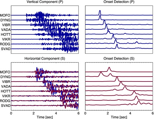
Vertical component (top left panel) and horizontal component (bottom left panel) waveforms and the corresponding STA/LTA onset signal (right-hand side) for a shallow seismic event from Askja, Iceland. The STA/LTA onset functions are calculated separately for each horizontal component, and then the S-wave onset functions are calculated from the rms summation at each time step of the two horizontal component onset functions. Note that the onset signals shown in the right-hand panels sometimes also have maxima other than the ‘correct’ phase arrivals, such as the prominent P arrival on the horizontal components of DYNG in the lower right panel: these do not matter because they are migrated away from the true coalescence point by the wrong look-up table (LUT) (in this case the S-wave LUT applied to the P-wave onset signal) and so neither contribute to the coalescence, nor bias the solution.
We define a continuous detection function fD(t), treating the specific case of fD(t) as the STA/LTA function. If y(t) is the recorded multicomponent signal, the requirement we place on fD(t) = f(y (t)) is that it returns a positive real scalar value. Polarization analysis of a multicomponent signal, array beamforming and other techniques can enhance the discrimination of specific phase arrivals such as P, SH and SV if it is desired to use these. These could be labelled explicitly as |$f_{D_P}(t), f_{D_{SH}}(t)$| and |$f_{D_{SV}}(t)$| and used with corresponding LUTs. We then establish an empirical relationship between fD(t) and the statistical uncertainty of the measured phase arrival time to derive the onset function fd(t), which represents the pdf for the phase arrival time pick.
The third and final step is to migrate the onset functions fd(t) back to every gridpoint in turn, for every time step, using the LUTs (see Section 2.2 for more details). Making the simplifying assumption that the traveltime errors in the forward model are independent, we apply a Bayesian formulation of traveltime inverse theory to develop a smoothing filter, which transforms the detection function fD into a phase arrival time pdf, fR, which describes both the picking and forward-modelling error. The backmigration is done using separate LUTs for each phase: in our case we use the vertical component of the seismic data to identify the onset function of the P waves and the horizontal components to map the S waves. To carry out the backpropagation as efficiently as possible, we make use of a multiresolution approach (described in Section 2.3). The resulting spatio-temporal maps represent the pdfs for hypocentres and origin times. We note that throughout most of the text we use the term ‘probability density’ loosely to refer to un-normalized probability density distributions.
2.1 Arrival onset detection
The STA/LTA function constitutes a form of noise normalization. Applied as an event detector, arrival detection is triggered when this function exceeds a given threshold. The threshold is chosen to achieve an acceptable number of true versus false triggers.
List of symbols.
| Univariate time-series/distributions and derived quantities: | |
| y(t) | Input time-series |
| fD(t) | Detection function, in the implementation here, the STA/LTA filtered trace of y(t) |
| fd(t) | Onset pdf representing the likelihood and uncertainty of traveltime picks (peaks at possible arrivals) |
| fr(t) | Theoretical phase arrival pdf, representing uncertainties due to both picking and forward modelling |
| fg(t) | pdf, representing the uncertainty of traveltime prediction (peaked at t = 0) |
| |$f_G(t)=\exp \left(\frac{-t^2}{2\sigma _G^2}\right)$| | Empirical pdf which can be convolved with fD(t) to generate fR(t) |
| fR(t) | Empirical phase arrival pdf, the width of Gaussians is stretched by factor α with respect to fr(t) |
| LD(t), Ld(t), LR(t) | Logarithms of above functions |
| tD | Local maximum of detection function, generally slightly delayed with respect to first-break pick |
| td | Local maximum of onset function, ‘pick time’ |
| ta | Actual arrival time of a phase (used for synthetic data in calibration procedure) |
| |$\sigma _D^2$| | Variance of Gaussian fitting a maximum of the detection function |
| |$\sigma _d^2$| | Variance of picking time due to noisy data |
| |$\sigma _g^2$| | Variance resulting from forward modelling |
| |$\sigma _r^2=\sigma _d^2+\sigma _g^2$| | Variance of arrival time due to combination of picking and forward modelling errors |
| |$\sigma _G^2=(\sigma _g^2-\sigma _A^2)/\alpha$| | Variance of Gaussian in fG(t) |
| |$\sigma _R^2\approx \frac{\sigma _r^2}{\alpha }$| | Variance of Gaussians in fR(t), determines resolution and robustness of coalescence |
| Multivariate distributions: | |
| |$F_d(T)=\prod f_{d_i}(t_i)$| | Multivariate pdf of onset times for arrivals at all stations and phase types |
| |$F_g(T|\vec{s}\,)$| | Multivariate pdf of forward modelled traveltimes for source location at |$\vec{s}$| |
| |$\hat{F}_g\left(T|\vec{s}\,\right)=F_g\left(T+T_g(\vec{s}\,)|\vec{s}\,\right)$| | Multivariate pdf expressing uncertainty of theoretical predictions centred around T = 0 |
| Location and coalescence: | |
| |$t_{g_i}(\vec{s}\,)$| | Forward modelled traveltime for hypocentre at |$\vec{s}$| |
| |$T_g(\vec{s}\,)$| | Vector describing traveltimes for all stations/phase types |
| t0 | (Putative) Earthquake origin time |
| |$f_c(t,\vec{s}\,)$| | Coalescence function describing the pdf of an event at origin time t and location |$\vec{s}$| |
| |$\hat{f}_C(t)$| | Maximum coalescence value of the spatial map at each time step |
| |$\hat{t}_0$| | Maximum likelihood event origin time (local maximum of |$\hat{f}_C(t)$|) |
| |$f_s(\vec{s}\,)$| | A posteriori pdf for location of one hypocentre (marginalization of fC over a short time window around |$\hat{t}_0$| |
| Δtrms | rms of arrival time residuals, describing the scatter of detection function maxima |$t_{d_i}$| around predicted times |$t_{g_i}$| |
| Empirical constants: | |
| |$\alpha ,\sigma _A^2$| | Slope and intercept of linear function relating variance of detection function and pick uncertainty (eq. 4) |
| User-settable parameters or parameters directly derived from user parameters: | |
| WS, WL | Short and long time window used by STA/LTA algorithm |
| Δt0 | Window length over which the marginalization of fC is performed to generate fs |
| Δtw | Window length for maximum value filter in multiresolution search |
| Δtx | Time interval required by seismic wavefront to pass a grid cell diagonally |
Notes: (i) All univariate functions can also be written with an index i enumerating all station/phase-type combinations.
(ii) pdf is used loosely to describe any un-normalized density function describing relative probabilities.
The variance estimate is dependent on the bandwidth of the signal and the choice of short window length WS; a good choice is one to two periods of the signal. We calibrate the relationship between the error in the observed arrival times tD, the variance |$\sigma _D^2$|, and the inverse of the logarithm of the SNR LD(tD) by adding synthetic signals to actually observed noise for a large range of SNRs. In the example in Fig. 3, the synthetic signal was generated by filtering a delta impulse at time ta with a fourth-order Butterworth filter with bandwidth 4–20 Hz (Fig. 3a). Only the amplitude and timing of the arrivals change; they are otherwise identical.
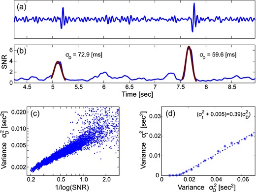
Example of model calibration for STA/LTA arrival onset function fD(t) for two arrivals. (a) Measured noise with synthetic arrivals superimposed. The signal bandwidth is 4–20 Hz. (b) STA/LTA trace fD(t) with an STA/LTA short window length of 0.15 s: red lines are Gaussian curves fitted to arrivals and their uncertainties σD. (c) Predicted uncertainties |$\sigma _D^2$| versus the inverse logarithm of the signal-to-noise ratio (SNR). (d) Observed picking error variance |$\sigma _d^2$| plotted against width squared of Gaussian fits to arrivals on onset trace |$\sigma _D^2$|. Even at very high SNR, where the picking error is essentially zero, the finite width of the signal results in a finite width of the Gaussian, determining the behaviour of the curve for |$\sigma _D^2<\,\sim\!0.015$| s2.
The maximum of fD(t), tD, is often later in time than the first time-break, that is, the idealized arrival time td. If the time-shift is the same for P and S detections, this does not affect the hypocentre determination, since all the arrival time estimates are offset in a similar way, but the origin time may be estimated slightly too late. If there is a systematic difference in the bias between P and S, then the use of station statics (see Section 3.2) is highly recommended to mitigate against a systematic effect on earthquake depth estimates.
Although the simple mapping between the width of the STA/LTA arrival onset function and the picking error worked well for our local and microseismic data sets, this assumption will need to be checked when applying the algorithm to data sets with different properties, for example, much larger-scale arrays. In any case, extension to more sophisticated detection algorithms is straightforward as long as any such mapping can be defined, even if it is approximate.
2.2 Coalescence microseismic mapping
The 4-D coalescence function can be reduced to two time-dependent outputs: the location as the instantaneous maximum of the spatial map |$\hat{s}(t)=\vec{s}@\mathrm{max}\left(f_C(t,\vec{s}\,)\right)$|, and the maximum value at each time step as |$\skew8\hat{f}_C(t)=f_C(t,\hat{s}(t))$|.
Leaving aside the scale factor α, the n-th root of |$f_C(t,\vec{s}\,)$|, termed the coalescence value, is the geometric mean of SNRs of the time-shifted individual STA/LTA traces, which have also been filtered (smoothed) to account for the forward modelling error (due to model uncertainties) and the error calibration. Computed continuously an event is triggered when the coalescence value exceeds a detection threshold: the time of the event |$\hat{t_0}$| is then set to the local maximum of the coalescence function |$\skew8\hat{f}_C(t)$| following the time at which the threshold is exceeded. The coalescence value provides a ranking of the events. The triggered events can be sorted by the coalescence value (SNR), with a subset of the data selected for subsequent analysis. The events with the best arrivals typically have the highest coalescence values. In this way the cut-off value in selecting events can be chosen interactively after processing, with the detection threshold not a critically important parameter of the algorithm.
The resultant map |$f_S(\vec{s}\,)$| represents the posterior pdf for the event hypocentre, subject to an unknown scaling factor. Estimates of the location and the location uncertainty are obtained by fitting a Gaussian function by least-squares at the local maximum of |$f_S(\vec{s}\,)$|. The parameters of the Gaussian function are returned as the mean location and three vectors describing the axes of a 3-D ellipsoid. If the distribution is multimodal, or otherwise non-Gaussian, then no simple error description is adequate and the location uncertainty can only be appreciated by inspection of the full map.
With the application of spatial weighting we can relax our earlier assumption that the search volume must be small with respect to the distance to the stations. With no prior knowledge of the errors in the forward model we might search for filtering functions |$f_G(t)=\exp(\frac{-t^2}{2\,\sigma _G^2})$| such that we achieve successful focusing of the coalescence function (see Section 2.3). Rather than searching for a separate |$\sigma _{g_i}$| corresponding to each station phase arrival, we instead search for two parameters, |$\sigma _{G_P}$| and |$\sigma _{G_S}$|, corresponding to the compressional and shear wave forward modelling errors, respectively. The spatial weighting in eq. (14) modifies |$f_{G_P(t)}$| and |$f_{G_S(t)}$|, albeit after convolution with |$f_{D_P(t)}$| and |$f_{D_S(t)}$|.
The search for filtering parameters |$\sigma _{G_{P,S}}$| is in essence similar to using the rms residual times (statistical error) as an estimate of the error in traveltime-based location methods. In a Bayesian framework this is only justified if no independent information about the quality of the velocity model exists. Otherwise, more reliable uncertainty estimates will be obtained by making use of any prior information about the quality of the model.
2.3 Multiresolution search
The search in time and space for events is implemented in discrete form. The required sampling is determined by the contributing signals |$f_{R_i}(t)$| and the spatial variation in modelled times, as governed by the geometry and velocity. The sharper the arrival times are resolved in |$f_{R_i}(t)$| the finer the sampling required in time and space to ensure that the solution is not missed. This assumes that the forward-modelled errors are accounted for by convolution with fG in eq. (11), and hence there exists a hypocentre where the signals will coalesce. Conversely, if the traces fR are smoothed heavily because of assumed large errors in the forward modelling or the arrival time detection, then the spatial and temporal grid can be more coarse.
Without a prior estimate of data and model misfit the algorithm might be used to undertake a search for the parameter σG of the Gaussian smoothing function fG(t). For normal distributions, we find that the value of |$\sigma _R^2=\sigma _D^2+\sigma _G^2$| that maximizes the coalescence function depends only on the statistic |$\Delta t_\mathrm{rms}=\sqrt{{\sum {(t_D - t_g)^2}/N}}$|, which is equivalent to the rms of the arrival time residuals (|$t_{D_i}$| are the maxima of the detection function |$f_{D_i}$| and |$t_{g_i}$| the corresponding theoretical arrival times). The coalescence function is maximized when |$\sqrt{(\sigma _D^2+\sigma _G^2)}=\Delta t_\mathrm{rms}$| (see Fig. 4). If σR ≪ Δtrms, the contributing signals |$f_{R_i}(t)$| are too sharp, and the signals no longer coalesce. On the other hand, if σR ≫ Δtrms, the coalescence region is spread over too wide a volume of the solution space resulting in loss of resolution. Because this increases the likelihood that unrelated arrivals will interfere with the solution, too large a value for σR can also result in biased solutions.
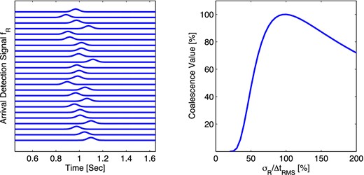
Synthetic data for a regular geometry of stations at 15° azimuthal increments. The arrival times have been perturbed by a random error with standard deviation Δtrms = 63 ms. The arrival signals fR, left, are modelled as Gaussian functions with standard deviation σR = Δtrms/2. Right shows the coalescence value at the event location as a function of σR. The coalescence value is maximimized when σR = Δtrms.
A possible strategy could thus be to vary σG as an additional parameter until the coalescence is maximized. Because any reduction in the required spatial and temporal sampling equates to an order-four reduction in computational cost, the additional cost of carrying out such a search on a small subset of the whole time series can be expected to pay off.
When detecting events we are primarily interested in finding the local maximum of |$f_C(t,\vec{s}\,)$| as the geometric mean SNR, eq. (14), not in estimating Δtrms. As the objective function is the sum of real scalar functions LR = log (fR), an upper bound to |$f_C(t,\vec{s}\,)$| over a time–space window can be established by summing the maximum values of LR over a time window Δtw at each gridpoint. Having determined that the upper bound of the function exceeds a threshold within a time–space window at a given sampling, the sampling is increased, thus constituting a form of Oct-Tree search. In applying the maximum value windowing function, it is necessary to have some idea of the residual times. If the search stops at too large a Δtw, in addition to the solution being under-resolved there is again the possibility of unrelated arrivals contributing to the solution. If the contributing signals |$f_{R_i}(t)$| are too sharp, that is, σR ≪ Δtrms, the coalescence will be lost as Δtw is reduced to Δtrms. In the ideal case when σR = Δtrms, the Oct-Tree search can progress until Δtw = 0.
3 PRACTICAL CONSIDERATIONS
3.1 The coalescence grid
Implementation of the CMM method requires choosing parameters that are appropriate for the dominant signal frequency, the spacing and areal extent of the seismic array and the target depth of events. The first step is to choose the window lengths for operation of the STA/LTA detector on the raw seismic signals. This is critical as it governs the successful discrimination of the arrivals. As a general rule, a short detection length that is sufficiently long to encompass one to two periods of the dominant signal frequency works well with a noise (long) window length of 3–10 times the short window length.
The second main consideration is the anticipated model and data misfit and the related choice in spacing of node points in the subsurface. The optimum node spacing is such that the time taken to travel the maximum diagonal distance between nodes is no more than about two-thirds of the signal duration in the contributing functions LR(t) used to calculate the coalescence function at each node (eqs 12 and 15). This in turn is controlled by the data (the dominant frequency of data and the short window length) and assumptions regarding the model data misfit.
There exists a trade-off between memory usage and computational cost on one hand and the need for sufficiently dense spatio-temporal sampling to represent the coalescence function and optimally resolve event locations. As the search is over a 4-D space, the sampling has a large impact on computational cost. The natural progression of the method is to first compute the coalescence function over the entire data set assuming a large σG, that is, nominally a large forward modelling error. This initial mapping only requires a coarse spatio-temporal sampling. Having established the approximate origin times and locations of events, we use these data to further refine the velocity model. Subsequent runs can be efficiently computed for a finer spatio-temporal sampling as we no longer need to search over the entire data set but can narrow down the spatial and temporal search to a volume that contains the events identified in the first iteration.
Finally, the simplest measure of the goodness of fit for each detected event is the coalescence value, that is, the geometric mean SNR of the signals contributing to the coalescence function, discussed here as the SNR of the seismic event. As we show later, comparison of the automatic CMM locations with those calculated from hand-picked arrivals enables a coalescence value (event SNR) to be chosen, which gives a similar population of events to the best that can be obtained by hand-picking arrivals.
Fig. 5 (top panel) shows the coalescence function at the time of the event for the shallow earthquake near Askja from which data are shown in Fig. 2. Fig. 5 (bottom panel) shows a map view and cross-section of the 3-D location probability volume, which is the marginalization (integration) of the coalescence function over a time window. Although the location is constrained by only a small number of seismometer stations, a clear coalescence signal is formed. The depth is poorly controlled because there are no seismometers directly above the event. Fig. 6 shows an expanded view of the location map and cross-section and also shows the grid of nodes at which the coalescence function was calculated. Rather than restricting the location estimate to a discrete grid node the best-fit hypocentral location can be derived from the maximum of a 3-D surface fitted locally to the 3-D coalescence volume.
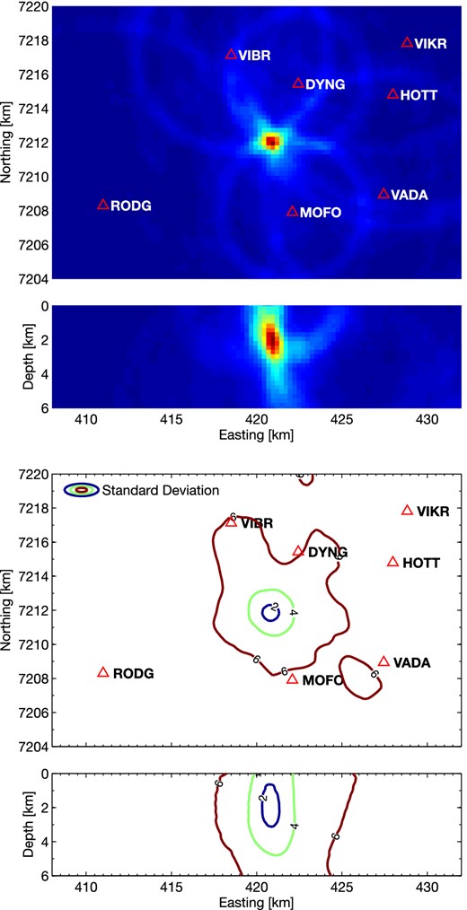
Map and elevation cross-sections of the coalescence function at the time of the event for the data from a shallow earthquake near Askja, Iceland, shown in Fig. 2. Red triangles show seismometer locations. The top two panels show the coalescence value at the time step corresponding to the origin time; the maximum value of this map corresponds to the maximum likelihood hypocentre of the event. The lower two panels show the marginalized pdf. The contours of the lower plots label the standard deviation of the pdf, as calculated after calibrating the input functions fD, Fig. 3.

Expanded view of map (top panel) and elevation cross-section (bottom panel) of the coalescence function shown in Fig. 5. The discrete spatial grid at which coalescence functions are determined is shown as dots.
We have used CMM extensively for local earthquake surveys in volcanic areas in Iceland. In Iceland, with a dominant signal frequency of 8–10 Hz, we find that values for the STA/LTA detector of 0.2 s/0.6 s work well. Using compiled Matlab code, a typical CMM run with 15 three-component seismometers, a sampling frequency of 100 sps, 400 000 nodes in the subsurface and 500 events per day runs approximately four times faster than real time on a single 2.67 GHz processor. So to analyse 1 yr's worth of data the algorithm can be run on 100 nodes of a cluster array, which takes approximately 1 day to complete. This method could be readily implemented as a real-time event detector on a single computer.
3.2 Station statics
Variations in near-surface structure and elevation, if not corrected for explicitly, cause station-specific delays which prevent the maxima of the |$f_{R_i}(t)$| functions from coalescing properly when migrated in the background model, limiting resolution and causing bias due to the fact that generally each event is recorded by a different set of stations. In traditional pick-based earthquake location algorithms, station correction terms can be estimated from the average residual at each station. As no explicit time picks are made in the CMM approach, a different approach is needed.
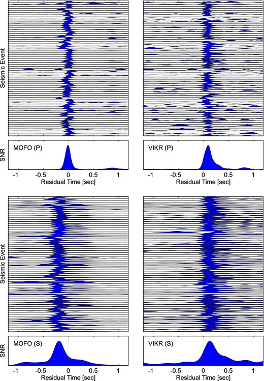
P-wave phase arrival functions for caldera events recorded at station MOFO and VIKR (upper plots), and S-wave arrival functions at these stations (lower plots). The geometric averages of the aligned signals are shown in the bottom panels. The maxima of these correspond to the maximum likelihood station correction terms.
The CMM procedure should then be repeated with traces time-shifted according to the static corrections, iterating if necessary. Even more accurate results can sometimes be obtained by introducing source area-specific station corrections, such as for shallow and deep events (see Lin & Shearer 2005 for this approach using traveltime based location algorithms).
4 DATA EXAMPLES
We show two examples of locating microseismicity produced by the injection of molten rock into the crust beneath Iceland (Fig. 8). The first is from a dyke injection in 2007 in the mid-crust near Upptyppingar, central Iceland (Martens et al.2010; White et al.2011). The second is from seismic activity associated with magma migration before and during the eruption of Eyjafjallajökull volcano in southern Iceland in 2010 March–May, which caused considerable disruption to air travel with the cancellation of over 100 000 flights in Europe (Tarasewicz et al.2011, 2012). In the latter case, over 20 000 events over a period of 14 d before the eruption were detected and located using CMM on data from an array of 14 seismometers: locating these many arrivals would have been unfeasible had all the arrival times been picked manually. In both examples, we carefully refined the traveltime picks of P- and S-wave arrivals manually for several hundred events and show the best locations using those arrival picks and double-difference relocations. We show that although there is some improvement in the manually relocated events, the main picture is produced from the automated CMM locations provided suitable event SNR cut-offs are used to remove the poorer locations.
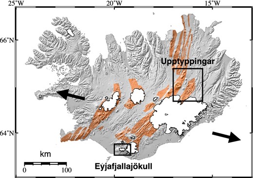
Map showing locations of areas in Iceland from which examples are drawn in this paper. Brown shaded areas are rift zones (after Einarsson & Sæmundsson 1987), and arrows show direction of plate spreading, which here is at a full rate of 20 mm a−1.
4.1 Upptyppingar dyke injection
The Upptyppingar dyke intrusion lasted almost a year during 2007–2008 and produced over 10 000 recorded microearthquakes, with local magnitudes mostly in the range 0–1 (Jakobsdóttir et al.2008). A local network of 27 three-component seismometers was used for making hypocentral locations and fault-plane solutions. The fault-plane solutions show that the failure planes are subparallel to the macroscopic dip of the dyke. They are interpreted as due to the fracture of plugs of solidified melt in the dyke, or as breaking a previously intruded dyke in the same location with the same orientation (White et al.2011).
Hypocentral locations of a subset of 540 microearthquakes with an average local magnitude of 0.9 generated during 2007 July 6–24 are shown in Fig. 9. They were chosen to be the set of earthquakes recorded by the permanent Icelandic SIL seismometer array maintained by the Icelandic Meteorological Office (Fig. 9a). The SIL array is much sparser in this region than was our temporary local array, although the SIL array does have eight seismometers within 50 km of Upptyppingar, so records earthquakes with a magnitude of completeness of 0.8. The manually refined and relatively relocated hypocentres from the SIL network define the plane of the dyke, dipping at 50°, with an rms misfit of 240 m to a single plane.
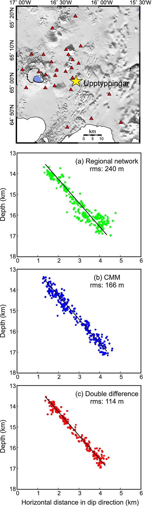
Map at top shows location of the earthquake swarm (yellow star) and seismometer stations (red triangles) near Upptyppingar, Iceland (see Fig. 8 for location). Panels show cross-sections looking along strike of the dyke intrusion with no vertical exaggeration of 540 microearthquakes during 2007 July 6–24: (a) after manual refinement and double-difference relocations of the SIL network data from eight stations; (b) located by automated CMM using local network of 27 stations; (c) after manual refinement of the traveltimes from local network of 27 stations, locations using Hypoinverse (Klein 2002), followed by double-difference relocation using HypoDD (Waldhauser 2001; White et al.2011). Assuming that the events lie in a single plane, the rms misfit to the plane is reduced from 166 m for CMM to 114 m after manual phase picking and double-difference relocation.
Automated CMM locations from the same set of 540 events are shown viewed along the strike of the dyke in Fig. 9(b). The rms misfit to a plane through the hypocentres is 166 m. Fig. 9(c) shows the same events, after we had made manual refinements of all the P- and S-wave arrival time picks. Hypocentres were first located using Hypoinverse (Klein 2002), and then their relative positions improved using a double-difference relative-relocation program (Waldhauser 2001). This reduced the rms misfit from a single plane to 114 m. Of course, we do not know whether this dyke did actually intrude along a single plane, or whether the seismic events were accurately located on the plane of the dyke. There is some reason to believe that the seismicity does indeed lie within the dyke because at these depths the Icelandic crust is normally ductile and aseismic. Seismicity is only produced by the high strain rates associated with melt intrusion. The melt intrusion itself would be along the dyke, and fluid mechanical and thermal considerations suggest that the dyke has a maximum thickness here of only about 1 m (White et al.2011). So the improvement in fit between CMM and the double-difference relocations is probably a real improvement in hypocentral locations.
However, the CMM locations themselves are already sufficiently good to constrain the dip of the dyke well, and the improvement after considerable manual intervention and relocation is relatively minor. To this extent, the CMM method is strongly validated.
4.2 Eyjafjallajökull eruption seismicity
Microseismic activity recorded during the 2 weeks before the eruption of Eyjafjallajökull began on 2010 March 20 was concentrated at depths of 3–6 km and was associated with the inflation of a magmatic intrusion beneath the east flank of the volcano (Tarasewicz et al.2012). Over 20 000 events during this period of intense activity were detected and located using CMM, and these provide a good demonstration of how the apparent scatter in locations varies with the event SNR (Fig. 10).
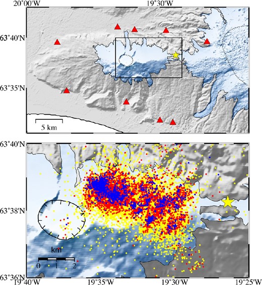
(Top panel) Map showing the closest seismometer locations (red triangles) around Eyjafjallajökull (see Fig. 8 for location); more distant stations were also used. Box shows outline of bottom map. (Bottom panel) Map view of over 20 000 CMM earthquake locations recorded during 2010 March 5–20 before the eruption of Eyjafjallajökull volcano in Iceland began on 2010 March 20. Events are colour coded by signal-to-noise ratio (SNR) for this parameter set in CMM: yellow events have 2.0 ≤ SNR ≤ 2.5; red 2.5 < SNR ≤ 3.5; blue SNR > 3.5. Grid-node spacing was 400 m. STA/LTA window lengths were 0.2 and 0.6 s, respectively. The data were bandpass filtered between 4 and 25 Hz. Yellow star shows location of fissure eruption on 2010 March 20, which preceded the main eruption from the summit crater (tick-marked outline) that began on 2010 April 14.
An appropriate event SNR (coalescence value) threshold must be chosen for any particular data set such that as many real events as possible are detected without large numbers of false ‘events’ being triggered. The actual value of the appropriate event SNR threshold may vary between data sets and between different parameter sets used. This is because the event SNR varies as a function of grid-node spacing, frequency filtering and choice of STA/LTA window lengths. An earthquake of the same magnitude may have different SNR depending on where it is located within the search grid: deeper earthquakes or those in sparser zones of the network may have lower coalescence values than if the same magnitude of earthquake occurred at shallow depths or in a denser part of the network.
In Fig. 10, the colour coding of the earthquake locations forms a concentric epicentral pattern with the highest-SNR events (blue) in the centre, radiating out to lower SNR values (red to yellow). In this case, is likely that all the blue earthquakes are well-located hypocentres, representing the largest-magnitude events. Red and yellow locations are likely to have smaller magnitudes or be less well located by comparison, with a higher incidence of false ‘events’ probable among the yellow locations. The concentric pattern suggests that it may even be the case that almost all events actually occurred in the region occupied by the blue, highest-SNR events, with the greater spread in red and yellow epicentres caused by location inaccuracy for smaller events.
In this example of tens of thousands of events, CMM's practical use was to give an overview of seismic activity and to produce rapidly a catalogue of earthquakes. CMM locations and event SNR values were then used to guide the selection of events for manual refinement and relative relocation. P and S arrival times were manually picked for a subset of 1400 earthquakes recorded at Eyjafjalljökull and located first in Hypoinverse (Klein 2002), then relatively relocated using HypoDD (Waldhauser 2001; Fig. 11). Comparison between CMM and Hypoinverse locations is a like-for-like comparison in the sense that both obtain single-event locations. HypoDD, which obtains relative relocations, should be expected to produce more tightly defined clusters (if indeed the seismicity was clustered) and is shown here as a ‘best-case’ set of locations.
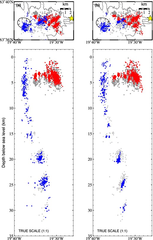
(a) Map view and east–west cross-section showing CMM earthquake hypocentres compared to Hypoinverse locations. Red dots are Hypoinverse (Klein 2002) locations for the same events whose CMM locations are shown in dark grey; blue dots are Hypoinverse locations for the same events with CMM locations shown in light grey. Dark grey/red events occurred before the flank eruption on 2010 March 20 (yellow star); these are a subset of the events in Fig. 10. Light grey/blue events were later, during the larger eruption from the summit crater (tick-marked outline) in April–May. The red/blue colouring differentiates in map view between the shallow, pre-eruption (red) events and the later, deep (blue) events. (b) Same as in (a), except red and blue events have been relatively relocated using HypoDD (Waldhauser 2001), which tightens the clusters.
To first order, CMM produces the same distribution of seismicity as manual single-event locations obtained in Hypoinverse (Fig. 11a). This is particularly the case for deeper events in this example. Mismatches in hypocentre locations are more pronounced in the shallow (<6 km) pre-eruption activity (red and dark grey in Fig. 11a). However, this is likely to be due in large part to Hypoinverse's treatment of station elevations using static corrections and the exclusion of some data in Hypoinverse where clear, discrete, arrival picks were not possible. These differences are exacerbated at shallow depths by the suboptimal geometry of the seismic monitoring network at Eyjafjallajökull (Tarasewicz et al.2011).
The relatively relocated hypocentres are generally more tightly clustered than the CMM and Hypoinverse picks (Fig. 11b). This is clearest in the clusters at >10 km depth (blue dots). This is not a fair comparison against CMM's single-event locations, but, as in the previous example, highlights the fact that our final ‘best’ set of manually refined and relatively relocated events is not radically different from the CMM locations obtained automatically.
5 CONCLUSIONS
The CMM method has proven to be a useful tool for locating hypocentres and origin times of local earthquakes. It is particularly helpful in regions of intense seismicity such as those that occur in volcanically active areas, in geothermal regions or in monitoring hydrofractures because it makes use of both P- and S-wave data to locate events without the risk of incorrect association of P- and S-wave picks, which can be a problem for automated schemes based on linearized inversion of discrete traveltime picks. It is robust against noise bursts on individual sensors because the apparent arrivals from them will generally be dispersed away from coalescence points and thus not contribute to the final location. The velocity model is amenable to being improved through introduction of complex 3-D velocity variations, of anisotropy or of variable Poisson's ratio.
The structure of the CMM method is such that it can be modified to include additional arrival phases such as horizontally or vertically polarized shear waves if they are present. It can also be extended to phase-pair analysis, which in principle brings it to similar resolution to that achievable by double-difference relocations [see Drew (2010) for more details]. Finally, the locations and predicted pick times returned by CMM can be used as starting points for more accurate but computationally intensive automatic pickers [e.g. MPX (Aldersons 2004); applied in combination with CMM by Lange et al.2012].
Seismic data used in this paper came from seismometers owned by Cambridge University; from those borrowed from the Natural Environment Research Council SEIS-UK (loan 842) (Brisbourne 2012); from the LOKI instrument pool, which is owned jointly by the Icelandic Meteorological Office, the Institute of Earth Sciences, University of Iceland and the Iceland GeoSurvey; and from the Icelandic Meteorological Office. We are grateful to all those who have worked in the field assisting in data collection, particularly Bryndís Brandsdóttir and Hilary Martens. Julian Drew was funded by Schlumberger and Jon Tarasewicz by an NERC studentship and CASE award supported by ERC Equipoise Ltd. Department Earth Sciences, Cambridge, contribution number ESC2857.
Now at: Schlumberger, Houston, USA.
Now at: Deutsches GeoForschungsZentrum - GFZ, Potsdam, Germany and Freie Universität Berlin.
