


Abstract
We propose new scaling laws for the properties of planetary dynamos. In particular, the Rossby number, the magnetic Reynolds number, the ratio of magnetic to kinetic energy, the Ohmic dissipation timescale and the characteristic aspect ratio of the columnar convection cells are all predicted to be power-law functions of two observable quantities: the magnetic dipole moment and the planetary rotation rate. The resulting scaling laws constitute a somewhat modified version of the scalings proposed by Christensen and Aubert. The main difference is that, in view of the small value of the Rossby number in planetary cores, we insist that the non-linear inertial term, | ${\boldsymbol u} \cdot \nabla {\boldsymbol u}$|, is negligible. This changes the exponents in the power-laws which relate the various properties of the fluid dynamo to the planetary dipole moment and rotation rate. Our scaling laws are consistent with the available numerical evidence.
1 INTRODUCTION
Estimated properties of those planets which are thought to have dynamos, along with the associated characteristic values of the Elsasser number, | $ \Lambda = {{\sigma B_z^2 } {/} { {\rho \Omega }}}$|, and the scaled magnetic field, | $ {{B_z} /{{\Omega R_C \sqrt {\rho \mu}}}}$|, based on the estimated mean axial field strength in the core. We use the crude estimates of λ ∼ 2 m2 s−1 and ρ ∼ 104 kg m−3 for the terrestrial planets, λ ∼ 30 m2 s−1 and ρ ∼ 103 kg m−3 for the gas giants (though estimates of λ for Saturn vary considerably) and λ ∼ 300 m2 s−1 and ρ ∼ 4 × 10³ kg m−3 for the ice giants.
| Planet | Rotation | Core | Dipole | Mean | Elsasser | Scaled |
|---|---|---|---|---|---|---|
| period (days) | radius, RC | moment, |${\boldsymbol m}$| | Bz in core | number | magnetic field | |
| (103 km) | (1022Am2) | (Gauss) | | $ \Lambda = \frac{{\sigma B_z^2 }}{{\rho \Omega }}$| | | $ \frac{{B_z }/ {\sqrt {\rho \mu }}} {{\Omega R_C }}$| | ||
| Mercury | 58.6 | 1.8 | 0.004 | 0.014 | 6 × 10⁻⁵ | 5.5 × 10⁻⁶ |
| Earth | 1 | 3.49 | 7.9 | 3.7 | 0.08 | 1.3 × 10⁻⁵ |
| Ganymede | 7.15 | ∼0.5 | ∼0.013 | ∼2 | ∼0.2 | ∼ 3.6 × 10⁻⁴ |
| Jupiter | 0.413 | 55 | 150,000 | 18 | 0.5 | 5.2 × 10⁻⁶ |
| Saturn | 0.444 | 29 | 4500 | 3.7 | 0.02 | 2.2 × 10⁻⁶ |
| Uranus | 0.718 | 18 | 390 | 1.3 | 10-4 | 1.0 × 10⁻⁶ |
| Neptune | 0.671 | 20 | 200 | 0.50 | 10-5 | 3.3 × 10⁻⁷ |
It is immediately apparent that Mercury, Uranus and Neptune have relatively weak magnetic fields with an Elsasser number, | $ \Lambda = {{\sigma B_z^2 } {/} { {\rho \Omega }}}$|, being very much less than unity, as indicated in Table 1. (Here σ is the electrical conductivity, ρ the fluid density and Ω the planetary rotation rate.) In all other cases, we find Λ = O(10− 1), possibly hinting at an order-of-magnitude balance between the Lorentz and Coriolis forces, sometimes called the strong-field regime. By contrast, Mercury, Uranus and Neptune, with their low Elsasser numbers, are often considered to operate in a weak-field regime (see, e.g. Rüdiger & Hollerbach 2004). It is important to note, however, that there are other ways in which the mean core magnetic field may be made dimensionless, and depending on the dimensionless grouping one uses, the fields of Mercury, Uranus and Neptune may or may not look anomalous. Compare, for example, the sixth and seventh columns in Table 1; in the final column it is Ganymede, rather than Mercury, Uranus or Neptune, that appears most out of line. Clearly, a more careful analysis is required before conclusions can be drawn about which dynamos are anomalous and which are not, and this provides part of the motivation for this study.
There has been a long tradition of trying to relate the dipole moments of the various planets, or equivalently their mean internal axial fields, to the observable properties of those planets and many of these scaling theories are discussed in the review by Christensen (2010). An early suggestion was that | $ \Lambda = {{\sigma B_z^2 }} {/} {{\rho \Omega }}\sim 1$| for all planetary dynamos, or in terms of the magnetic energy per unit mass, | $ {{B_z^2 }} {/} { {\rho \mu }}\sim \lambda \Omega$|, where λ is the magnetic diffusivity. Leaving aside Mercury's particularly weak magnetic field, and the idiosyncratic ice giants, Table 1 suggests that there may be some merit to this hypothesis, though there is not much variation in rotation rate between the Earth, Jupiter and Saturn, so this is not a very stringent test.
An alternative and largely successful approach is that of Christensen & Aubert (2006), Christensen et al. (2009) and Christensen (2010). The hallmark of Christensen's scaling laws is the assertion that Ω, although a crucial catalyst for dynamo action, is ultimately unimportant when it comes to determining the magnitude of the saturated, steady-on-average magnetic field. Rather, the saturated magnetic energy density, B2/ρμ, should be determined by the rate of working of the buoyancy force which drives the dynamo. There is solid support for this assertion from numerical dynamo simulations (see Christensen 2010, and references therein) and so we embrace this hypothesis, using it to full advantage in the analysis that follows.
Our starting point, however, is somewhat different. It is an empirical observation that the mean axial vorticity in rapidly rotating turbulent convection is (more or less) independent of the background rotation rate. As we shall see, this is equivalent to Christensen's suggestion that the magnetic energy density in saturated dynamos is determined by the rate of working of the buoyancy force and independent of Ω (except to the extent that Ω may influence the rate of working of the buoyancy force). Starting from this single assumption we deduce, from first principles, a number of scaling laws which are shown to be consistent with the available numerical and observational evidence.
2 REVISITING THE HYPOTHESIS THAT THE MAGNETIC ENERGY IS DETERMINED BY THE RATE OF WORKING OF THE BUOYANCY FORCES
There have been many attempts to arrive at a scaling law for the magnetic energy density in planetary dynamos. Typically, one starts with an assumed force balance in the core, which in turn leads to scaling laws for the characteristic velocity and for B2/ρμ. However, in some cases the assumed force balance has the non-linear inertial term, | $ {\boldsymbol u} \cdot \nabla {\boldsymbol u}$|, as an order-one quantity (see the review by Christensen 2010), which is an assumption we wish to avoid. Nevertheless, as noted above, there is strong numerical support for the hypothesis that the saturated magnetic energy density in planetary dynamos is primarily determined by the rate of working of the buoyancy force and is very nearly independent of Ω (except to the extent that Ω may influence the rate of production of energy by the buoyancy forces). Consequently, we take a rather different approach here and decouple the question as to whether or not B2/ρμ is independent of Ω from any assumed velocity scaling in the core. Let us start by considering why B2/ρμ might be independent of Ω.
As we shall see, the energy production term on the left of eq. (5) is proportional to the radial heat flux out of the core, and because the mantle provides the dominant thermal resistance to heat flow (at least in the terrestrial planets), that heat flux is independent of the dynamics of the core, and hence of Ω. It follows that the left-hand side of eq. (5) should be independent of the background rotation rate. We conclude, therefore, that the magnetic energy density does not depend on Ω provided that the magnitude of the small-scale vorticity is itself independent of Ω, and indeed this is consistent with the rotating convection experiments of Kunnen et al. (2010), though these experiments have values of Ro somewhat larger than in a planetary core: u/Ωℓ ∼ 10− 3 → 10− 1. In any event, it is the presence of the rate of working of the buoyancy forces and the apparent absence of Ω in eq. (5) which provides independent motivation for the hypothesis that, in the saturated state, | $ {{B^2 } / {\rho \mu }}$| is determined by the energy generation rate and does not exhibit any explicit dependence on the magnitude of the background rotation. Of course, these arguments are somewhat tenuous, yet when combined with the strong numerical evidence that | $ {{B^2 } / {\rho \mu }}$| is controlled only by the production of energy by buoyancy forces (Christensen 2010), it provides some motivation to explore the consequences of the hypothesis that | $ {{B^2 } / {\rho \mu }}$| is independent of the rotation rate.
We must, however, add one caveat to these statements. It has become common in some dynamo simulations to prescribe the temperature difference across the core, rather than prescribe the radial heat flux. In such a situation the heat flux, and hence the rate of working of the buoyancy forces, may be influenced by Ω, and as a result there may be an implicit dependence of | $ {{B^2 } / {\rho \mu }}$| on Ω. Of course, such a dependence is an artefact of the boundary conditions used in those particular simulations. Nevertheless, from time to time we shall want to invoke the results of the numerical simulations to test our scaling laws. Consequently, when we refer below to | $ {{B^2 } / {\rho \mu }}$| being independent of Ω, we really mean that any influence of Ω on | $ {{B^2 } / {\rho \mu }}$| occurs only though its indirect influence on the rate of working of the buoyancy forces, an influence that should vanish when fixed-flux boundary conditions are used.
In this paper, we restrict ourselves to low-| $ {\rm Pr} _m$| dynamos and so use eq. (8) rather than eq. (9). In principle, the theory developed below could be generalized to include dynamos in which | $ {\rm Pr} _m$| is not small by multiplying P, or equivalently qT, by | $ f( {Pr _m ,Ro} )$|. However, because the functional form of | $ f( {{\rm Pr} _m ,Ro})$| has yet to be determined (it is almost certainly not a simple power law), and planetary cores invariably satisfy | $ {\rm Pr} _m \ll 1$|, we shall leave aside most questions as to the role of | $ {\rm Pr} _m$| in those dynamos for which | $ {\rm Pr} _m$| is not small.
Note that, so far, we have not assumed any particular scaling for | $ u = | {\boldsymbol u} |$|, as the logic above rests solely on the assumption that | $ {{B^2 } / {\rho \mu }}$| is independent of Ω and is a function of P and ℓ alone. This is important because the scaling for u has proven to be a subtle issue over which there is some disagreement. (Some of the scalings which have been proposed for u are based on the assumption that | $ {\boldsymbol u} \cdot \nabla {\boldsymbol u}$| is an order-one quantity, which seems improbable for most planetary dynamos in the light of the extremely low value of Ro.) We shall return to the issue of how u scales shortly.
Consequently, we might tentatively accept eq. (8) as an empirically established relationship which can be rationalized through the observation that the small-scale vorticity in rapidly rotating turbulent convection is more or less independent of Ω. We can then ask what other scaling laws follow from eq. (8) when combined with the requirement for a force balance in the core. Let us, therefore, explore this force balance.
3 THE CORE FORCE BALANCE AND RESULTING SCALING LAWS
The key result here is eq. (15), which fixes the Rossby number. Equation (13), which gives the ratio of magnetic to kinetic energy, and eq. (14), which can be rewritten as Rm = ΛRo− 1/2, are simply rearrangements of eqs (15) and (8), and so cannot be regarded as independent predictions. However, scaling eq. (12) for the ratio of the two integral scales can be considered as an additional prediction. Combining eqs (12) and (15) yields | $ {u / {\ell _ \bot }}\sim {\rm P}^{1/3} \ell _{//}^{ - 2/3}$|, and so our model predicts that the large-scale vorticity is independent of the background rotation, which is a result to which we shall return shortly.
Equation (15) might be compared with Christensen's proposal of | $ Ro\sim ( {{{\rm P} / {\Omega ^3 \ell _{//}^2 }}})^{1/3}$|, based on the assumption that | $ {\boldsymbol u} \cdot \nabla {\boldsymbol u}$| plays a significant role, or with the other common estimates of | $ Ro\sim ( {{{\rm P} / {\Omega ^3 \ell _{//}^2 }}} )^{1/2}$| and | $ Ro\sim ( {{{\rm P} / {\Omega ^3 \ell _{//}^2 }}})^{2/5}$|, all of which are discussed in detail in Christensen (2010). We shall test eq. (15) against the numerical simulations in Section 4, where we shall see that it is an excellent fit to the data.
Note that the diffusivities λ and ν play no role in this scaling theory, except to the extent that λ appears in the definition of Rm. This is, of course, typical of turbulent motion in which the diffusivities are small: the key dynamic processes are controlled by the large-scale dynamics which do not normally depend on the diffusivities, provided that those diffusivities are sufficiently small.
A number of interesting observations stem from eqs (19) and (20). First, we note that | $ {u / {\ell _ \bot }}$| is the characteristic large-scale vorticity associated with the columnar convection rolls, | $ \omega _{{\rm large}} \sim {u / {\ell _ \bot }}$|. On the other hand, we know from Section 2 that | $ {\lambda / {\ell _{\min }^2 }}$| is associated with the small-scale vorticity, | $ {\lambda / {\ell _{\min }^2 }}\sim \omega _{{\rm small}}$|. It follows from eq. (19) that ωlarge ∼ ωsmall, which is the hallmark of 2-D turbulence (Davidson 2004) and might also be expected to hold in highly anisotropic turbulence in which ℓ// ≫ ℓ⊥. Moreover, self-consistency of the model demands that we must extend the requirement that ωsmall does not depend on the background rotation rate to the stronger constraint that | $ \omega _{{\rm large}} \sim {u / {\ell _ \bot }}$| is also independent of Ω.
Empirical scaling laws for the dependence of | $ \tau _\lambda ^ *$| and | $ \tau _\lambda ^\Omega$| on Ro and Rm have been determined by several authors, most recently by Christensen (2010), Yadav et al. (2012) and Stelzer & Jackson (2013), based on analysing a multitude of numerical experiments. This provides yet another test of our predicted scaling laws.
Third, eq. (20) highlights a potential difficulty which arises from the modest value of Rm in the core of the terrestrial planets, and the consequent lack of a separation of scales. For example, in the Earth we have u ∼ 0.2 mm s−1 and Ro ∼ 10− 6. It follows that | $ R_m = {{u\ell _{//} } / \lambda }\sim 200$| and | $ {{\ell _{//} } / {\ell _ \bot }}\sim {\rm 30}$|, at least according to eq. (12), and so eq. (20) yields | $ {{\ell _{\min }^{} } / {\ell _ \bot ^{} }}\sim ( {{{u\ell _ \bot } / \lambda }} )^{ - 1/2} \sim 0.4$|. Evidently, in practice, it is not always easy to distinguish between the smaller of the two integral scales, ℓ⊥, and the microscale ℓmin . Nevertheless, it is important to make the distinction from a conceptual point of view as ℓ⊥ and ℓmin are predicted to scale in very different ways, at least for large Rm. Note also that, for the Earth, uℓ⊥/λ and uℓmin /λ are both predicted to have values close to unity, that is, uℓ⊥/λ ∼ 7 and | $ {{u\ell _{\min } } / \lambda }\sim 3$|.
4 TESTING THE SCALING LAWS
Of course, estimates eq. (12) → eq. (15), as well as eqs (22) and (23), must be treated with caution, as there could be a multitude of length scales in the core, some associated with convection rolls, others with boundary layers, and yet others with internal shear layers and current sheets. In the scaling analysis above we simply scale all the forces on two integral scales, ℓ// ∼ RC and ℓ⊥, which we might associate with the axial and transverse dimensions of the columnar convection rolls. Nevertheless, we are free to ask if these scaling laws are consistent with what we know. The answer, by and large, is yes, at least to the extent that we can estimate the parameters involved.
Fig. 1 shows that data of Christensen & Aubert (2006) along with prediction of eq. (15). On the left is the full data set, corresponding to | $ 0.06 < {\rm Pr} _m < 10$|, whereas on the right only data in the range | $ 0.06 < {\rm Pr} _m < 1$| is shown, which is closer to the low-| $ {\rm Pr} _m$| regime of interest here. It is clear that eq. (15) is indeed a good fit to the data for | $ {\rm Pr} _m < 1$|. So there is strong numerical support for our prediction of n = 4/9 in eq. (24).
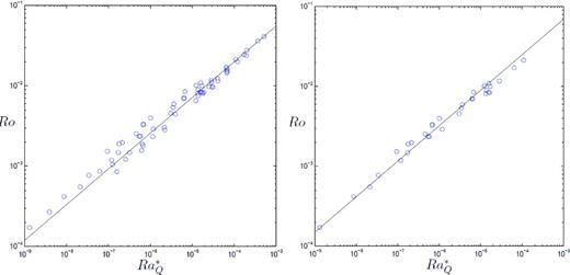
Computed values of Ro versus | $ Ra_Q^* = {{\rm P} {/} {\Omega ^3 D^2 }}$| taken from the data set of Christensen & Aubert (2006). (a) The full data set, | $ 0.06 < {\rm Pr} _m < 10$|. (b) A restricted data set, | $ 0.06 < {\rm Pr} _m < 1$|. Power-law eq. (15) is shown for comparison.
These are close to the empirical observations of Yadav et al. (2012), who estimate | $ \tau _\lambda ^\Omega \sim Ro^{ - 0.8}$|, and by implication | $ \tau _\lambda ^ * \sim {{Ro^{1/5} } / {R_m^{} }}$|, for numerical dynamos with slip boundary conditions. Moreover, eq. (27) is close to the estimate of Christensen (2010) who, based on the evidence of many numerical experiments, suggests that | $ \tau _\lambda ^ *$| scales approximately as | $ \tau _\lambda ^ * \sim {{Ro^{1/6} } / {R_m^{} }}$|, which in turn implies | $ \tau _\lambda ^\Omega \sim Ro^{ - 5/6}$|.
The differences between the theoretical prediction, | $ \tau _\lambda ^ * \sim {{Ro^{1/4} } / {R_m^{} }}$|, and the two empirical estimates, | $ \tau _\lambda ^ * \sim {{Ro^{1/5} } / {R_m^{} }}$| and | $ \tau _\lambda ^ * \sim {{Ro^{1/6} } / {R_m^{} }}$|, are modest, differing as they do by factors of Ro1/20 and Ro1/12, respectively. Given that the variation in Ro is limited to three decades in the numerical experiments, and that the scatter in the data leaves some uncertainly in the exponent for Ro, one cannot readily use the numerical evidence to distinguish between the various proposed scaling relationships. Nevertheless, the fact that | $ \tau _\lambda ^ * \sim {{Ro^{1/5} } / {R_m^{} }}$| and | $ \tau _\lambda ^ * \sim {{Ro^{1/6} } / {R_m^{} }}$| are both reasonable fits to their respective numerical data sets does at least tell us that eq. (27) must also be reasonably in line with that data. Yet another estimate of | $ \tau _\lambda ^ *$|, again based on the evidence of numerical simulations, is that of Stelzer & Jackson (2013) which, leaving aside any | $ {\rm Pr} _m^{}$| dependence, suggests | $ \tau _\lambda ^ * \sim {{{Ro}^\alpha } / {R_m^{} }}$|, 0.09 < α < 0.11. This is somewhat more at odds with our prediction of | $ \tau _\lambda ^ * \sim {{{Ro}^{1/4} } / {R_m^{} }}$|, and this discrepancy remains to be accounted for. (The discrepancy possibly arises from the fact that the estimate | $ \tau _\lambda ^ * \sim {{Ro^{0.1} } / {R_m^{} }}$| is a curve fit over a relatively wide range of | $ {\rm Pr} _m^{}$|, specifically | $ 0.06 < {\rm Pr} _m < 33$|, whereas our prediction is for low | $ {\rm Pr} _m^{}$| only.)
In addition to the evidence of the numerical simulations, we might note that eqs (13) and (14) are consistent with what we know about the Earth, where we have Ro ∼ 10− 6 and Rm ∼ 200 (see Section 3). For example, estimate eq. (14) combined with eq. (15) suggests Λ ∼ 0.2, which is in line with Table 1, where Λ is estimated as Λ ∼ 0.08. Also, eq. (13) combined with eq. (15) suggests | $ {{( {B^2 /\rho \mu } )} / {u^2 }}\sim 10^3$| which, given that u ∼ 0.2 mm s−1 in the core, suggests a mean core field strength of B ∼ 7 Gauss. This is also in line with Table 1 where the mean axial field strength based on the dipole moment |${\boldsymbol m}$| is estimated to be Bz ∼ 4 Gauss.
In summary, then, prediction eq. (15) for the scaling of the Rossby number, as well as predictions eqs (22) and (23) for the scaling of the normalized Ohmic dissipation time, are all reasonably consistent with the evidence of the numerical experiments. Moreover eqs (13) and (14), which predict the ratio of the magnetic to kinetic energy and the magnetic Reynolds number, are consistent with what we know about the geodynamo. The success of eq. (15) also lends support to eqs (13) and (14), because these are simple rearrangements of eqs (15) and (8).
5 PREDICTIONS FOR OTHER PLANETS
Fig. 2 shows that data of Christensen & Aubert (2006) for Ro versus | $ {{B_{{\rm rms}} } / {\Omega D\sqrt {\rho \mu } }}$|, along with prediction eq. (28). (Note that D is the thickness of the fluid shell.) On the left is the full data set, corresponding to | $ 0.06 < {\rm Pr} _m < 10$|, whereas on the right only data in the range | $ 0.06 < {\rm Pr} _m < 1$| is shown, which is closer to the regime of interest. Note that the characteristic field strength used by Christensen & Aubert (2006) is the rms magnetic field in the core, rather than the mean axial field calculated from eq. (1). However, provided there is not a strong Ω effect, the two fields should be of similar magnitudes. It seems that eq. (28) is not out of line with the numerical data, but the fit is somewhat disappointing when compared with Fig. 1. In some ways this is curious, because eq. (28) simply combines eqs (8) and (15) and Fig. 1 shows that eq. (15) is an excellent fit to the data. We conclude that the scatter in Fig. 2 comes mostly from estimate eq. (8). It is likely that the discrepancy arises from the use of data in which | $ {\rm Pr} _m \sim 1$|, rather than | $ {\rm Pr} _m \ll 1$|, which necessitates the use of eq. (9) rather eq. (8) to estimate the magnetic energy density. The problem, of course, is that we do not know the functional form of | $ f( {Pr _m^{} ,Ro} )$| in eq. (9).
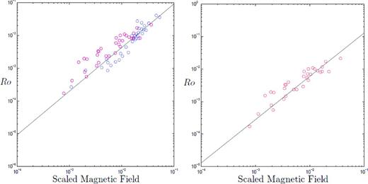
Computed values of Ro versus | $ {{B_{{\rm rms}} } {/} {\Omega D\sqrt {\rho \mu } }}$| taken from the data set of Christensen & Aubert (2006). (a) The full data set, | $ 0.06 < {\rm Pr} _m < 10$|, with | $ {\rm Pr} _m < 1$| coloured red and | $ {\rm Pr} _m > 1$| coloured blue. (b) A restricted data set, | $ 0.06 < {\rm Pr} _m < 1$|. Power-law eq. (28) is shown for comparison.
If one has sufficient confidence in power-law eq. (28), it is tempting to use it to estimate Ro, and hence | $ {{\rm P} {/} {{\Omega ^3 \ell _{//}^2 }}}$|, in the core of the planets, although this is a rather substantial extrapolation. In any event, the various estimates of | ${{B_z {/} {\Omega R_C} \sqrt {\rho \mu }}}$| are tabulated in Table 2 and they are surprisingly consistent across the different planetary dynamos (except, perhaps, for Ganymede). Expression eq. (28) then suggests Rossby numbers in the range Ro ∼ 10− 9 → 10− 6, as shown in Table 2.
| Planet | | $ \frac{{{{B_z } / {\sqrt {\rho \mu } }}}}{{\Omega R_C }}$| | | $ Ro = \frac{u}{{\Omega R_C }}$| | | $ \frac{{{{B_z^2 } / {\rho \mu }}}}{{u^2 }}$| | | $ \frac{{\ell _{//} }}{{\ell _ \bot }}$| | | $ R_m \sim \frac{\Lambda }{{Ro^{1/2} }}$| |
|---|---|---|---|---|---|
| Mercury | 5.5 × 10⁻⁶ | 1 × 10⁻⁷ | 3 × 10³ | 60 | 0.2 |
| Earth | 1.3 × 10⁻⁵ | 3 × 10⁻⁷ | 2 × 10³ | 40 | 140 |
| Ganymede | ∼ 3.6 × 10⁻⁴ | ∼ 3 × 10⁻⁵ | ∼200 | ∼10 | ∼40 |
| Jupiter | 5.2 × 10⁻⁶ | 1 × 10⁻⁷ | 3 × 10³ | 60 | 1600 |
| Saturn | 2.2 × 10⁻⁶ | 3 × 10⁻⁸ | 6 × 10³ | 80 | 130 |
| Uranus | 1.0 × 10⁻⁶ | 1 × 10⁻⁸ | 1 × 10⁴ | 100 | 1.2 |
| Neptune | 3.3 × 10⁻⁷ | 2 × 10⁻⁹ | 2 × 10⁴ | 140 | 0.3 |
Given these estimates of Ro we can explore the predictions of scaling laws eq. (12) → eq. (14) for planets other than the Earth, though there is an implicit assumption here that the dynamos in these planets are qualitatively similar to those of the numerical simulations that provide support for eqs (8) and (15). In any event, the tentative results of these scaling laws are shown in Table 2. For simplicity, we have taken the pre-factors in eqs (12), (13), (14), (15) and (28) to be unity, so little weight should be given to the precise numerical values. Three immediate observations are that: (i) for all of the planets, the predicted magnetic energy density in the core swamps the kinetic energy by a factor of ∼ 103; (ii) the convection is predicted to be strongly anisotropic; and (iii), the magnetic Reynolds number for Saturn is surprisingly low, closer to that of the Earth than that of Jupiter. (Actually, there is some evidence that Saturn's dynamo may have a different structure to that of the other planets, as discussed in Cao et al.2012). However, perhaps the primary observation is that Mercury, Uranus and Neptune appear not to fall into our scaling regime, as their predicted values of Rm are much too low to sustain dynamo action. Once again, we are led to the conclusion that the dynamos of Mercury, Uranus and Neptune are somehow anomalous.
There is, however, a possible explanation for Mercury's apparently anomalous behaviour. The prediction | $ R_m \sim {\Lambda / {Ro^{1/2} }}$|, combined with eqs (1) and (28), leads to | $ R_m \ {\propto} \ \Omega ^{ - 1/3} B_z^{4/3} R_C^{2/3} \sim \Omega ^{ - 1/3} | {\boldsymbol m} |^{4/3} R_C^{ - 10/3}$| and so, for a given Ω and |${\boldsymbol m}$|, the predicted value of Rm is extremely sensitive to the assumed core radius, or shell thickness if we take ℓ// ∼ D. If, as suggested by Christensen (2006) and Christensen et al. (2009), only the innermost regions of Mercury's core are in convective motion, then the effective values of RC or D may be very much less than their nominal values. Moreover, | $ R_m \propto D_{}^{ - 10/3}$| tells us that reducing D by a factor of, say, 4 would increase the predicted value of Rm by a factor of 100. It remains to be seen as to whether or not this can account for Mercury's low value of Rm in Table 2.
6 CONCLUSIONS
We have developed new scaling laws based on Christensen's hypothesis that the saturated magnetic energy density should not depend on the planetary rotation rate. However, these scaling laws are different to those of Christensen (2010) and others because, in the light of the very small value of Ro in planetary cores, we insist that the non-linear inertial term, | $ {\boldsymbol u} \cdot \nabla {\boldsymbol u}$|, is neglected in the core force balance. Our predictions are consistent with what we know about the Earth, at least to the extent that we can test them. Also, our predicted scalings for the Rossby number and dimensionless Ohmic dissipation time, | $ Ro\sim ( {{{\rm P} / {\Omega ^3 \ell _{//}^2 }}} )^{4/9}$|, | $ \tau _\lambda ^ * \sim {{Ro^{1/4} } / {R_m^{} }}$| and | $ \tau _\lambda ^\Omega \sim Ro^{ - 3/4}$|, are reasonably consistent with the results of the numerical simulations shown in Christensen & Aubert (2006), Christensen (2010), Yadav et al. (2012) and Stelzer & Jackson (2013). When applied to planets other than the Earth, our scalings suggest that the magnetic fields of Mercury, Uranus and Neptune are anomalous. This conclusion for Uranus and Neptune is hardly surprising, given their complex magnetic field structure and large dipole inclination. In the case of Mercury there are two possibilities; either the dynamo operates in a different regime, or else it is confined to a small part of the fluid core, as suggested by Christensen (2006).
The author thanks Andy Jackson and Eric King for helpful comments and Andrea Maffioli for help in preparing the manuscript.
