


Abstract
We present 3-D models of the P- and S-wave velocity distributions in the crust and uppermost mantle beneath Sicily, Calabria (Southern Italy), and surrounding submerged areas, obtained by tomographic inversion of traveltimes of regional body waves phases. Our method combines double-difference tomographic inversion with a post-processing procedure [Weighted Average Model method (WAM)]. This procedure was applied to a set of models consistent with the experimental data. We tested the ability of the WAM procedure to mitigate the uncertainty associated with the arbitrary nature of the many input parameters required for each inversion. The local reliability and resolution of the obtained models have been assessed through: synthetic tests, experimental tests carried out with independent data sets and unconventional tests based on the analysis of the internal consistency of the P- and S-velocity models. The tomographic images provide a detailed sketch of P- and S-wave velocity anomalies. These clearly show the shape of the Sicilian-Maghrebian belt beneath Sicily and Calabrian Arc at different depths. Low VP and Vs bodies are imaged beneath Stromboli and Marsili volcanoes in the southern Tyrrhenian, whereas high and low seismic velocities alternate beneath the Etna giving inferences on the possible depth of the mantle melting feeding the volcano. In the upper crust, the main sedimentary basins and tectonic features are also well imaged. Finally, tomographic cross sections show the trend of the Moho in the study area, where its depth ranges between 35 and 40 km beneath the Sicilian belt and between 15 and 22 km in the southern Tyrrhenian basin and Ionian Sea.
1 INTRODUCTION
The morphological reconstruction of geological structures at lithospheric scale and the physical and tectonic characterization of the Sicilian and surrounding areas are steps necessary for understanding the geodynamic evolution of the whole Mediterranean region (Casero & Roure 1994; Catalano et al.2000; Monaco et al.2002; Giunta et al.2009). In the last decades, many studies based on local earthquake tomography (LET) have been performed to define the velocity fields of P and S seismic waves in the crust and upper mantle, beneath the Sicilian-Apennine system (Di Stefano et al.1999, 2009; Neri et al.2002; Barberi et al.2004; Scafidi et al.2009; Orecchio et al.2011). Although the velocity models proposed by these authors have been resulted useful for describing the main features of the region, their reliability and resolution are still insufficient to discriminate structures at regional and local scale in the complex geodynamic context of the studied area. The aim of this work is to expand the knowledge of the crustal structures (down to 40 km depth) of the Calabrian-Sicilian-Tyrrhenian region. This will be done building new 3-D models of body wave seismic velocity (VP and Vs) distributions and assessing their reliability.
Our VP and Vs models were obtained in two steps. First, we calculated a set of models compatible with selected experimental data using double-difference seismic tomography (DD tomography; Zhang & Thurber 2003) with different sets of input parameters. Subsequently, we applied the Weighted Average Model (WAM) post-processing method (Calò 2009; Calò et al.2011, 2012) to improve the reliability and detail of the final models. The high reliability and resolution of the models developed in this work will enable us to make hypotheses on composition and physical state of the main underground structures.
1.1 Geological setting
The Sicilian area is located in the central western Mediterranean Sea along the Africa–Europe Plate boundary (Fig. 1). Convergence between the two continents began in the Late Oligocene-Early Miocene after the counter clockwise rotation of the Corsica-Sardinia block and its collision with the African margin (Bellon et al.1977; Channel et al.1979; Dercourt et al.1986).
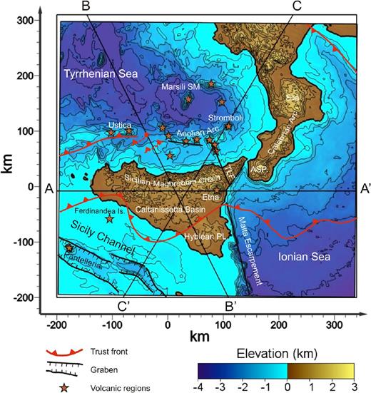
Topographic map of the study region reporting the main tectonic and geographic elements. The black lines (A–A′, B–B′ and C–C′) are the traces of the tomographic vertical sections shown in Fig. 12. TFL is the Tindari-Letojanni strike-slip system whereas ASP is the Aspromonte mountain.
The dominant element of the study area is the collisional complex of Sicily. It involves; (i) a SE vergent thrust belt, up to 15 km thick, consisting of a ‘European’ element (Peloritan Units), a ‘Tethyan’ element (Sicilide Units) and an ‘African’ element (Maghrebian Sicilian Units; Catalano & D'Argenio 1982; Roure et al.1990; Lentini et al.1994; Catalano et al.1996, 2000; Finetti 2005; Accaino et al.2007). These units are supposed to lie on an undeformed crystalline basement. They outcrop in the Sicily land and are submerged in the surrounding areas; (ii) A northwestern dipping foredeep, partially buried by the Gela thrust system and extending onto Malta platform (Ogniben 1969; Grasso 1997; Lickorish et al.1999); (iii) a foreland area outcropping in southeastern Sicily (Iblean Plateau) submerged by the Sicily Channel and Ionian Sea.
The Peloritan Units are part of the Peloritan–Calabrian Arc that connects the NW–SE trending Apennines with the E–W Maghrebide chain of Sicily (Fig. 1). The southeastern margin of Sicily is bounded by the Malta Escarpment and its system of normal faults (Bianca et al.1999; Giunta et al.2004; Adelfio et al.2006; Billi et al.2007). This latter represents the transition between the continental domain and the Ionian Sea (Casero & Roure 1994; Nicolich et al.2000) where various authors (Catalano et al.2000, and references therein) suggest the transition to ocean crust.
Sicily Channel Sea surrounds the southern Sicily coast. It is underlain by the Pelagian platform, which includes the outcropping Iblean Plateau, the submerged Malta and Pantelleria grabens and the Malta Plateau. Sicily Channel is marked by a tectonic stress different with respect to the rest of the study area. Many authors (Boccaletti et al.1984; Finetti & Del Ben 1986; Argnani et al.1989; Corti et al.2006) suggest that this area is a result of extensional-transtensive tectonics documented by a thinned continental crust and by the presence of the Malta and Pantelleria grabens, and marked by large magnetic and gravimetric anomalies (Della Vedova et al.1989).
To the north, Sicily is bordered by the Tyrrhenian Sea. Subduction of the Ionian slab and lied on a thinning of the Sicilian-Tyrrhenian continental lithosphere (just at north and west of the coastlines of the Sicily and Calabria, respectively) and on the formation of a backarc oceanic crust off the shore of the Aeolian archipelago (Kastens et al.1988; Argnani 2000; Chironi et al.2000; Sartori 2003). The subduction of the Ionian slab is evidenced by a narrow Wadati-Benioff zone, plunging from the Ionian Sea towards the southern Tyrrhenian basin below the Calabrian Arc (Caputo et al.1970, 1972; Malinverno & Ryan 1986; Anderson & Jackson 1987; Giardini & Velona 1991; Selvaggi & Chiarabba 1995; Cimini & Marchetti 2006; Calò et al.2012).
In the study area, several variations of the Moho depth are documented. The deepest estimation of Moho depth (37–38 km) are recognized beneath the thrust belts under Northern Sicily (Cassinis et al.1969; Colombi et al.1973). The Moho depth decreases towards the submerged areas. In the Southern Tyrrhenian, the Moho depth ranges from around 25 km close to the coastline to 8–10 km beneath the Marsili Basin, whereas in the Ionian Sea ranges from 20 to 16 km (Giese & Morelli 1975; Catalano et al.2000; Nicolich et al.2000).
There are various active volcanic regions in the Sicilian area, including, going from north to south: the Marsili Seamount, located in the Southern Tyrrhenian and representing a volcanic-arc edifice emplaced on an older, ‘relict’ backarc (Ventura et al.2013); the backarc Aeolian Archipelago related to the Ionian subduction (Peccerillo 1985; Ellam et al.1988); the Etna volcano located in the eastern part of Sicily and related to local mantle upwelling because of differential flexure of the same Ionian subduction (Doglioni et al.1999; Nicolich et al.2000); the Pantelleria island (Rotolo et al.2006; Civile et al.2008) and the Isola Ferdinandea (currently submerged) located in the Sicily channel and related to the extensional stress presented in the area (Caracausi et al.2005).
1.2 Seismicity
The study area is affected by crustal and deep seismicity, mostly localized in two main seismogenic volumes (Giunta et al.2004; Adelfio et al.2006; Billi et al.2007). The deep seismicity, marked by hypocentral depth between 40 and 500 km, is concentrated in the eastern sector of the southern Tyrrhenian. This seismic activity is related to the subduction of the Ionian slab beneath the Calabrian Arc (Chiarabba et al.2005 and references therein). The shallow seismicity (hypocentral depth less than 40 km) mainly occurs because of the brittle deformation both of the submerged and emerged part of the Maghrebian chain (Neri et al.1996; Giunta et al.2004; Sgroi et al.2012) and the volcanic activity associated with Mt. Etna, the Aeolian Islands. Another component of the whole shallow Sicilian seismicity consists of the earthquakes localized in the foreland area (i.e. Caltanissetta basin, Sicily channel and southeastern Sicily).
Seismicity of the Sicilian area can be further subdivided into minor subsets containing either strictly interdependent events (i.e. seismic clusters) or independent events (background seismicity). Seismic clusters are characterized by high spatial and temporal hypocentral density. A high-resolution analysis of some relevant clusters of this area (Giunta et al.2009; Giorgianni et al.2012) highlights the presence of several active faults marked by different extensions and focal mechanisms.
2 DATA SETS
In this work we used the P- and S-phase arrival times extracted from the ‘Bollettino Sismico’, edited by the INGV (Istituto Nazionale di Geofisica e Vulcanologia). Data refer to earthquakes recorded by the National Seismological Network from 1981 January to 2009 December. INGV operators manually review the picking of the main phases. The data set was updated with arrival times, not included in the INGV catalogues, picked out on waveforms recorded from some temporary arrays, installed in the Sicilian area during the major seismic crises (e.g. the sequences of Pollina in 1993 and Palermo in 2002).
We selected the events with epicentre in the area between 35° and 40°N of latitude and 11° and 17°E of longitude and hypocentral depth less than 100 km, recorded by at least 10 stations and located by the INGV with a RMS <0.5 s. For each event, the mean amount of P- and S-arrival times resulted of 16.3 and 6.9, respectively. Earthquakes in the southern Tyrrenian, Sicily, and Calabria regions were selected with an azimuthal gap less than 180 degrees. However in some boundary of the Sicily Channel and of the Ionian Sea the events with azimuthal gap less than 250° were also included to increase the data coverage.
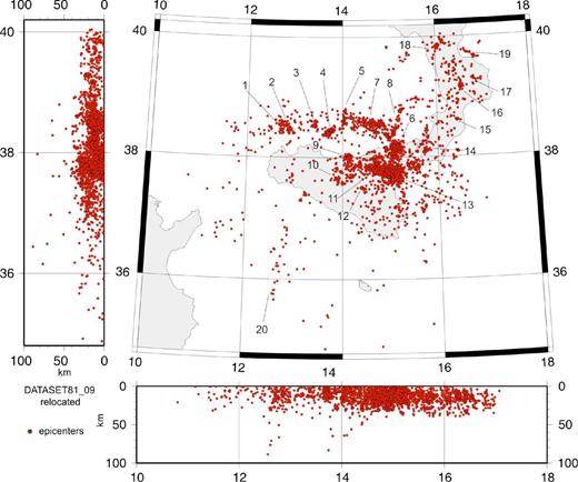
As the hypocentral locations reported by the INGV bulletin are determined using the same 1-D P- and S-velocity models for the whole Italian region (Chiarabba et al.2005), we relocated the selected earthquakes using the code HypoInverse2000 (Klein 2002) and two 1-D models (M1 and M2; Fig. 3) optimized for the study area (Capizzi et al. 2001; Giunta et al.2004).
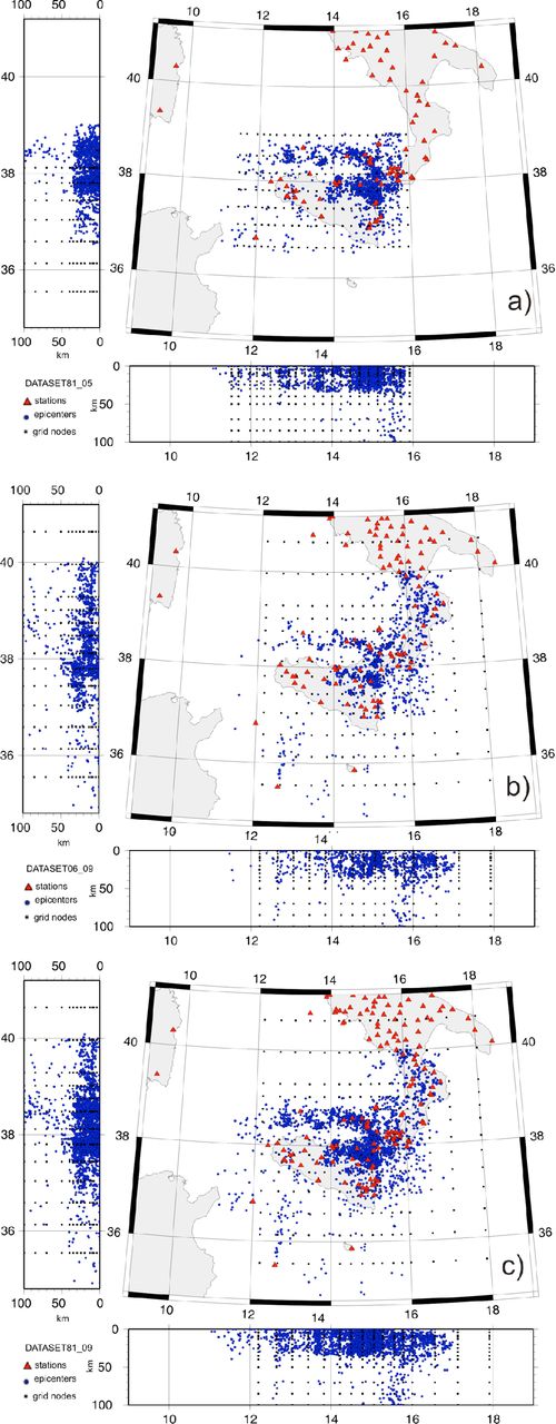
Projections of the hypocentres relative to the data sets 81_05 (a), 06_09 (b) and 81_09 (c) on a horizontal plane and on vertical planes oriented SN and WE. The black dots in the maps represent the nodes of the reference inversion grids and the red triangles the locations of seismic stations.
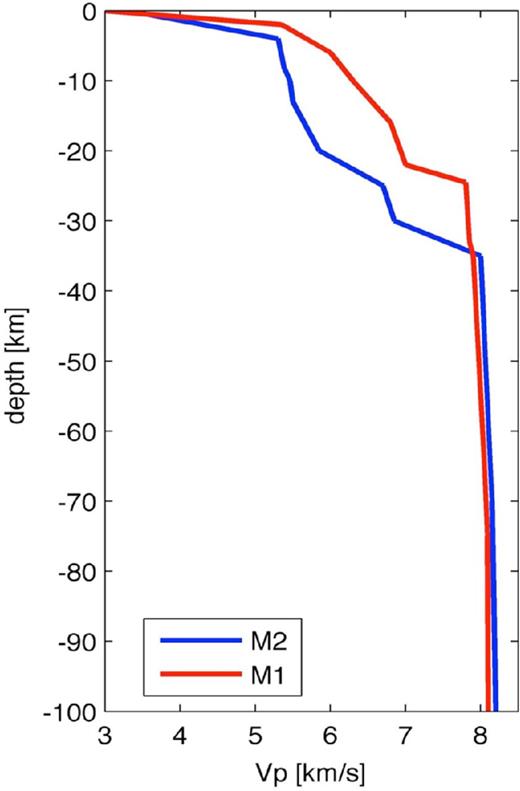
VP starting models M1 and M2 used in this work. For both models the initial Vs model is equal to VP/1.78.
The DD tomographic inversion code of Zhang & Thurber (2003) jointly inverts absolute and differential arrival times to determine seismic velocity distributions and hypocentral parameters. Differential arrival times can be calculated from both waveform cross-correlation techniques for similar waveforms and absolute arrival times catalogue (Waldhauser & Ellsworth 2000). In this work, all the differential arrival times are determined from the catalogue of absolute arrival times.
Selected data were used to build three sub-data sets to perform assessment tests and study the dependency of the final velocity models by the experimental information (see Sections 3 and 4). The first data set (81_05, Fig. 2; Table 1) contains 1954 earthquakes occurred in the period from January 1981 to December 2005 and consists of 31 270 P and 13 588 S absolute arrival times recorded by 192 seismic stations, supplemented by 73 022 P and 27 893 S differential times. The second data set (06_09; Fig. 2; Table 1) includes 1494 earthquakes occurred from January 2006 to December 2009 and contains 27 668 P and 11 183 S absolute arrival times recorded by 140 seismic stations. The differential times are 63 246 and 29 683 for the P- and S-waves, respectively. It is worth noting that the events related to the two data sets (81_05 and 06_09), cover areas with different extension and are relative to different time intervals. The investigating volume is approximately the same for both data sets although only one of them (06_09) has a more homogeneous event distribution. We performed some assessment tests with the two data sets that will be described in the Sections 4.2 and 4.3. Finally, we built the third data set (81_09; Fig. 2; Table 1), relative to 3445 earthquakes, by merging the two previous ones. Fig. 4 shows the projection of the source-station straight lines relative to the P phases of the data set 81_09 on a horizontal and N–S and W–E vertical planes.
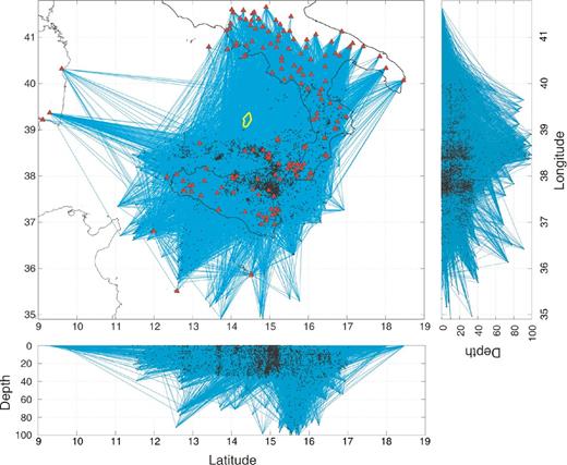
P-wave ray paths for the data set 81_09 traced for a homogeneous medium. In yellow is reported the position of the Marsili seamount.
Parameters of the three data sets used in this work (81–05, 06–09 and 81–09). For each data set is reported: the number of events (Events), the absolute (Abs) and differential (Diff) P and S times, the initial average root mean square (RMS) and final ones (WAMRMS), the initial and final standard deviations (std), the mean absolute horizontal and vertical (Δh and Δz) displacements of the hypocentres and their standard deviations (HWSTD).
| Data set | Events | Abs P | Abs S | Diff P | Diff S | Stations | Initial mean RMS (s) | Final | Δh (km) | Δz (km) |
|---|---|---|---|---|---|---|---|---|---|---|
| WAMRMS (s) | ||||||||||
| 81_05 | 1951 | 31 270 | 13 588 | 73 022 | 27 893 | 192 | 0.3 | 0.2 | 1.86 | 3.5 |
| (std 0.16) | (std 0.01) | (HWSTD 2.5) | (HWSTD 3.5) | |||||||
| 06_09 | 1494 | 27 668 | 11 183 | 63 246 | 29 687 | 140 | 0.24 | 0.1 | 1.47 | 3.34 |
| (std 0.1) | (std 0.04) | (HWSTD 1.94) | (HWSTD 3.35) | |||||||
| 81_09 | 3445 | 56 225 | 23 858 | 11 9866 | 49 261 | 189 | 0.28 | 0.09 | 1.44 | 3.1 |
| (std 0.14) | (std 0.04) | (HWSTD 0.11) | (HWSTD 3.04) |
3 CONSTRUCTION OF VP AND Vs MODELS
To obtain a 3-D seismic velocity model from local earthquake data inversion, a large set of parameters must be assigned a priori. These affect: (i) the parametrization of the initial velocity models, (ii) the algorithms for the ray paths and traveltime calculation, (iii) the rules for data selection, (iv) the relative weighting of different data when they are integrated in simultaneous inversions, (v) the strategy of the iterative inversion procedure, (vi) the damping of the inversion algorithm, etc. In the tomographic problem, even small variations of these parameters generate changes on the inversion results. Often, the perturbations thus produced on the models, although small in relative value, can be sufficient to lead to different geological interpretations.
In this work, for each data set, we first ran the tomoDD code (Zhang & Thurber 2003) to solve the VP and Vs structures and hypocentral locations. Then the post-processing WAM method (Calò 2009; Calò et al.2011) was applied to obtain more reliable final models.
3.1 Setup of the double-difference velocity models
At first we calculated models of VP and Vs using a reference set of input parameters for tomoDD code. This was empirically optimized for the study area by following the procedures suggested in literature. Afterwards we performed several inversions by varying the parameters of this set in compliance with the criteria described below and reported in Appendix A. For the three data sets the a priori optimal average node spacing of the inversion grid is about 35 km in the horizontal directions and 7 km in the vertical one (Fig. 2; Appendix A). The origin of the Cartesian coordinate system was centred at 14°E, 37.8°N and 0 km of depth. The iterative procedure for most of the tomographic inversions was setup assigning larger weights to the absolute data in the first cycles, to roughly determine the P- and S-waves velocities distributions and higher weights to the differential data in the last cycles, to improve the model resolution and the relative hypocentral locations inside and around the seismogenic volumes. Furthermore, we alternated joint inversions (VP, Vs and hypocentres) and only hypocentral location in most of the inversions. For all the iterations, initial velocity values at nodes characterized by derivative weight sum (DWS; Toomey & Foulger 1989) less than 10 were not included in the inversion. The DWS parameter is a measure of the amount of experimental information used to estimate the velocity at each node of the inversion grid. Damping values required for the damped least-square solution were established to maintain at each iteration, values of Condition Number (Paige & Saunders 1982) between 50 and 70.
For each data set we performed several inversions adopting different node-grids and weighting data schemes as reported in Appendix A. Furthermore, we performed some inversions by varying the initial velocity models (2–5 per cent of the reference models M1 and M2) and for the data set 81_09 we also calculated three inversions using a schematic 3-D initial model (M3, Appendix A). The M3 initial model was constructed assigning the velocity distribution M1 to the Tyrrhenian region (38.2°N–40°N, 11E–15.8E) and M2 to the remaining area. Among the whole set of inversions we selected 19, 20 and 15 models (we will refer to them as DD models) for the data sets 81_05, 06_09 and 81_09, respectively (Appendix A). All these models were selected to obtain a sampling of the space of the models as homogeneous as possible and in agreement with the experimental data.
3.2 WAM procedure
The 54 VP and Vs models selected among all the DD inversions (reported in Appendix A) were re-sampled in a common Cartesian grid (WAM grid; Calò 2009). The origin of the WAM grid has been located at 14°E, 37.8°N and 0 km depth. Its size is 540 × 510 × 100 km3 in X, Y and Z directions, respectively. Horizontal and vertical spacing are 3 and 2 km, respectively. Corresponding DWS values were also interpolated in the nodes of the same grid.
In the WAM method the final velocity distribution is a weighted average of velocity estimates assigned to each WAM node. The weight of each velocity value is a function of the corresponding DWS value. Zhang & Thurber (2007) showed that it is generally reasonable to use the ray-sampling density (DWS) to approximately describe the spatial distribution of the model resolution. In this work the WAM velocity distributions are based only on seismic velocities calculated on nodes with DWS > 100.
By means of the WAM technique, we constructed three VP and Vs WAMs, mod81_05, mod06_09 and mod81_09, for the corresponding data sets using 19, 20 and 15 DD models, respectively. Moreover, the WAM, mod81_05_09, was build using the 39 velocity distributions relative to the data sets 81_05 and 06_09. These models will be discussed in Section 4.2 to validate the effectiveness of the WAM method. Finally, we constructed the WAMs using the whole set of 54 DD velocity inversion results (mod54P and mod54S). To assess the inversion stability, the WAM method also allows associating a weighted standard deviation (WSTD) to each node of the WAM grid. Details on the WSTD distributions obtained in this work are reported in Appendix B. Finally, we have calculated the WAM hypocentres, using as weighting factor the final rms values of the events relative to each inversion.
4 ASSESSMENT TESTS
4.1 Checkerboard tests
We performed two synthetic tests using the 81_05 and 06_09 data sets. We calculated traveltimes in VP and Vs models that alternate high positive and negative anomalies with similar pattern to that of the checkerboard test of Zhao & Kanamori (1992). We added Gaussian distributed noise with a standard deviation of 0.1 and 0.2 s to the P and S traveltimes (Zeiler & Velasco 2009). Thus, the double-difference tomographic technique and the WAM post-processing were applied to recover the checkerboard velocity models.
For the first test, we used a model involving patches with regular horizontal size of 30 km and vertical size ranging between 2 and 10 km (Fig. 5) overlapping the model M1. The patches have, alternately, velocity values ±6 per cent with respect to the 1D model. This model was used to calculate the traveltimes corresponding to the data set 81_05. It is worth noting that this velocity distribution, with strong vertical gradients to depths of 15–35 km, was useful to assess the resolution in transition regions marked by high vertical velocity gradients as the Moho and Conrad discontinuity.
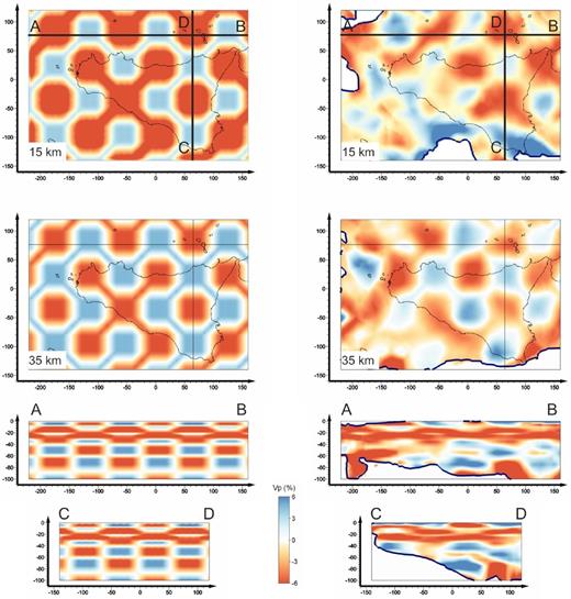
Synthetic test performed using the data set 81_05. Checkerboard model used to calculate the synthetic traveltimes (left side) and model recovered after the WAM procedure (right side). Only the parts of the model marked by DWS > 100 are shown. Horizontal sections are at 15 and 35 km of depth. Black lines (A–B, and C–D) in the horizontal maps are the traces of the vertical slices.
For the second test, we used a model with patches irregular both in horizontal and vertical dimensions overlapping the model M2 (Fig. 6). Size of checkerboard structures ranges from 20 to 50 km in the horizontal dimension and from 2 to 20 km in the vertical one. Anomalies of the patches are alternately ±5 per cent with respect to the 1-D velocity model. This model was used to calculate the traveltimes corresponding to the data set 06_09.

Synthetic test performed using the data set 06_09 Checkerboard model used to calculate the synthetic traveltimes (left side) and model recovered after the WAM procedure (right side). Only the parts of the model marked by DWS > 100 are shown. Horizontal sections are at 15 and 35 km of depth. Black lines (A–B and C–D) in the horizontal maps are the traces of the vertical slices.
Fig. 5 shows the P-wave velocity anomalies recovered by the WAM procedure applied to the synthetic data set 81_05. The horizontal slices at 15 and 35 km of depth show that the velocity anomalies are well recovered. Vertical sections show that the thin structures at depth of 15–35 km are also sufficiently reconstructed. Horizontal and vertical sections suggest that a good resolution down to a depth of 40 km is expected. Fig. 6 reports the results of the test performed using the data set 06_09. Also in this test the horizontal patches at depth of 15 and 35 km are sufficiently recovered in most of the investigating volume although a slight underestimation of the absolute velocity values is observed at shallow depths. Vertical sections show a satisfactory reconstruction of the patches down to 50 km. Both tests suggest that the selected data sets are adequate to reconstruct velocity structures with horizontal size of 20–50 km and 2–10 km of thickness at least down to depth of 40–50 km, when our procedure is used. In particular the test performed with the data set 81_05 showed that strong vertical velocity gradients, incorporated into the model to reproduce the major lithospheric discontinuities, are sufficiently imaged using only this data set. Checkerboard models reconstructed using synthetic traveltimes of the S-phases provided similar results.
Considering the results obtained with the two data sets (81_05 and 06_09), a synthetic test performed using the whole data set (81_09) will certainly provide a reconstruction of the velocity patterns equal or greater. For this reason, this test was considered unnecessary.
4.2 Comparison of the experimental velocity models
In this section, we compare the 54 DD velocity models (Appendix A) and four experimental WAMs (mod81_05, mod06_09, mod81_05_09 and mod81_09).
To quantify the overall dissimilarity between two models, we calculated the average of DPGlm(i) at the nodes marked by DWS > 100 in both models. First, we compared the DPG values of the 1431 pairs of models relative to the 54 DD inversions. The DPG mean value resulted 6.8 per cent and for some pairs the DPG exceeded 14 per cent. However, the largest velocity anomalies observed in the models, are significantly larger than the average DPG. This suggests that in any case they are reliably recovered. In Fig. 7 four examples of DD velocity models are reported: two calculated using the data set 81_05 (Figs 7a and b), and two calculated with the 06_09 one (Figs 7c and d). The DPG values of the two pairs of models obtained from the same data set are 6 and 4.7 per cent, for the data set 81_05 and 06_09, respectively, whereas those related to different data sets are 9.5 and 10.8 per cent. DPG values of pairs of models related to different data sets resulted, as expected, on average significantly higher than those related to models obtained with the same data set.
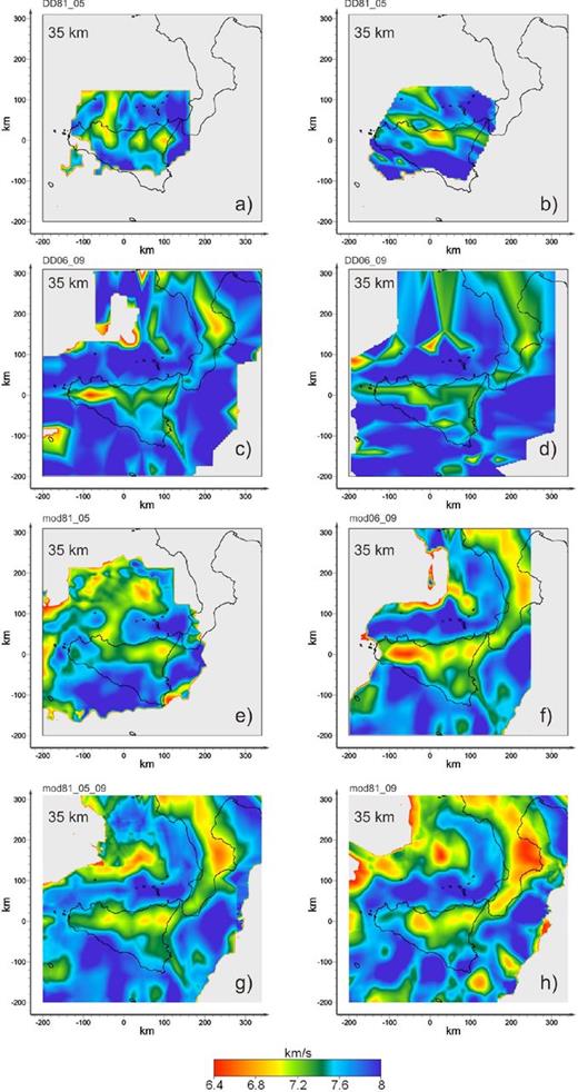
Horizontal sections at 35 km depth of representative DD models and intermediate WAMs. Only the parts of the models marked by DWS > 100 are shown; (a) DD VP model calculated using the data set 81_05 and reference inversion grid (N01 in Appendix A); (b) DD VP model obtained using a grid rotated of 60° counter-clockwise (N06 in Appendix A); (c) DD VP model calculated with the 06_09 data set and reference inversion grid (N26 in Appendix A); (d) DD VP model obtained using a grid rotated of 60° counter-clockwise (N23 in Appendix A); (e) Equivalent section of the WAM mod81_05; (f) Equivalent section of the WAM mod06_09; (g) Equivalent section of the WAM mod81_05_09 calculated using 39 standard DD models; (h) Equivalent section of the WAM mod81_09 calculated using 15 standard DD models.
This test shows that, although the size of the two data sets seems a priori large enough to solve this tomographic problem their stand-alone amount of information is not adequate for a reliable reconstruction of the velocity anomalies. In fact, even if the large-scale velocity anomalies result in rather similar trends, absolute velocity values and shape of the smaller structures are not sufficiently constrained for unambiguous characterization of the geological framework of the study area.
After processing the models with the WAM method, the DPG for the pair mod81_05-mod06_09 was 4.3 per cent with the largest values not exceeding 5 per cent in few border areas of the common region. Although the agreement between these two models is significantly greater than that of two generic DD inversions, the differences between the velocity distributions are still excessively large for an unambiguous definition of the geological structures of the area.
Figs 7(e) and (f) represent the horizontal VP section at depth of 35 km of mod81_05 and mod06_09. Despite some portions of the velocity distributions appear rather different, most of the anomalies located in the central part of the investigated volume have similar pattern. In our models, the central part of the models is always characterized by the highest values of DWS. Consequently, we imputed the main contribute of the discrepancy between the two models to the insufficiency of the value 100 as the minimum threshold of the DWS parameter. This statement will be taken into account in the test described in Section 4.3. Finally, we calculated the DPG between the WAMs mod81_05_09 and mod81_09. The mean value resulted less than 3 per cent and the highest one did not exceed 4 per cent. The horizontal slices of the two VP models at depth of 35 km are reported in Figs 7(g) and (h) and show that shape and absolute values of the velocity distributions are very similar. The strong similarity of these two models suggests that the problem related to the substantial lack of experimental information may be overcome through a gradual update of the model by applying the WAM method. Furthermore, this feature of the WAM procedure may represent also a way to overcome problems related to the computational burden of large sets of data in tomographic imaging. The same analysis was performed also for the Vs distributions providing analogous results.
Finally, as above mentioned, we constructed our final VP and Vs models unifying the results of the 54 single inversions and thus mod54P and mod54S represent the most complete WAMs that we have calculated. Fig. 8 reports a map imaging the number of the VP models used to calculate the velocity estimates at a depth of 5 and 35 km, respectively. The comparison of these maps with the VP ones (Figs 7 and 11) highlights the necessity to have at least 10 models sampling the same region to calculate WAM velocity values sufficiently reliable.
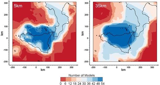
Horizontal sections at 5 and 35 km depth showing the number of DD models used to calculate the P-wave seismic velocities with the WAM method.
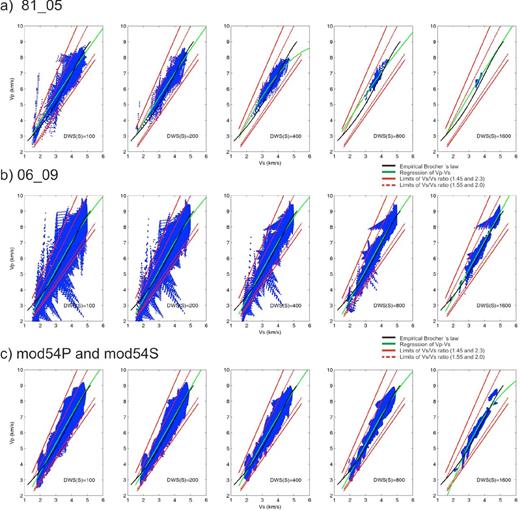
Plot of VP against Vs values for different DWSS thresholds for: (a) DD model obtained after the inversion of the data set 81_05, (b) 06_09 DD model and (c) for the final WAMs (mod54P and mod54S). The DD models were re-sampled in the WAM grid to be consistent with the amount of values reported in figures.
Horizontal and vertical projections of the relocated hypocentres and averaged with the WAM method. The numbers identify the seismic clusters discussed in the text.
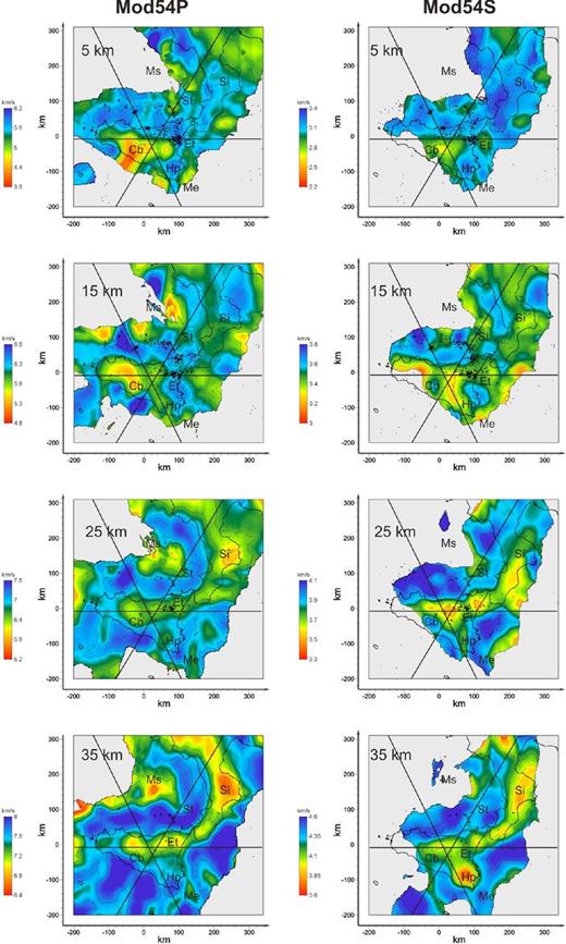
Horizontal sections of mod54P (left) and mod54S (right) at 5, 15, 25 and 35 km of depth. Only the part of the models with DWS > 200 are displayed. Black dots represent the relocated earthquakes projected onto the horizontal slices within ±5 km. Contour lines of the seismic velocities are of 0.5 km s−1 and 0.25 km s−1 with respect to the mean value of the corresponding VP and Vs sections, respectively. Legend: Cb, Caltanissetta basin; Ms, Marsili Seamount; St, Stromboli; Si, Sila; Et, Etna; Hp, Hyblean Plateu; Ma, Malta escarpment.
4.3 VP–Vs correlation
Relationships between VP, Vs and density of the rock, provide the basic relationships for the joint interpretation of different types of seismic and, eventually, Bouguer anomaly data. These relationships were proposed and progressively improved by several laboratory measurements (Birch 1966; Carmichael 1989; Henkel et al.1990; Christensen & Mooney 1995; Brocher 2005). We performed a correlation analysis between the VP and Vs distributions referred to models obtained with the same data set and input parameters set, to verify their correlation degree and the consistency with the empirical laws proposed by Brocher (2005).
Zhang & Thurber (2007) showed that the parameter DWS is related to the local resolution of the inversion and thus it could be used to delimit the well-resolved areas. However, the choice of a threshold to define the volumes within which the tomographic estimates are enough reliable is not straightforward, being dependent on the complexity of the studied geological system.
Figs 9(a) and (b) show the diagrams of VP–Vs dispersion relative to two single DD inversions of the data sets 81_05 and 06_09, respectively. These distributions are representative of the inversions carried out with the two data sets. For both sets of inversions we calculated the VP–Vs distributions using DWS thresholds for Vs estimates (DWSS) corresponding to the values of 100, 200, 400, 800 and 1600. We considered the parameter DWSS because in our work it is always lower than DWSP (DWS for VP estimates). In the same plots, the curves of the empirical Brocher's relationship (Brocher 2005, black line) and of the VP–Vs best fit calculated in a least-square sense (green lines) are reported. The straight lines VP = (1.47)* Vs and VP = (2.3)*Vs, plotted in red, are reported as limits for a realistic empirical correlation law because they refer, respectively, to the values 0.1 and 0.38 of the Poisson's ratio and these can be considered reasonably extremes for the lithospheric rocks (Christensen & Mooney 1995; Christensen 1996 and references therein). Figs 9(a) and (b) show that DWSS greater than 100 enclose volumes marked by estimates of VP and Vs highly dispersed around the regression curves. This dispersion is much larger than that one expected from measurements on rock samples. Therefore it can be mainly attributed to an insufficient experimental constraint in the resolution of the inverse problem. It is worth noting that the regression curve is not significantly different from the Brocher's empirical relation. This suggests that the errors affecting the velocity values are randomly distributed and with mean close to zero. Furthermore, the trend does not change significantly for higher DWSS thresholds, although the dispersion of the estimates around the regression curves is greatly reduced.
The test suggests a DWSS threshold of 200 for the inversions performed with the data set 81_05, whereas only velocities calculated with DWSS greater than 800 are satisfactory for the inversions with the data set 06_09. Hence, a conservative value of the DWSS threshold (e.g. greater than 500) should ensure a reduction of the velocity spreading and consequently a decreasing of the mismatching between the empirical law and experimental VP–Vs distribution. This will result useful for the interpretation of the absolute seismic velocities but not indispensable on the recognition of important geological structures at regional scale because of the strong reduction of investigated volume.
The empirical Brocher's law (2005) is the result of thousands of observations of VP and Vs compiled for a wide variety of lithospheric rock samples. The data for each law calculated with our velocity values show coherent deviations from the global regression law. Furthermore, this analysis allows us to observe a slight deviation of the regression curve from the Brocher's law. This deviation is negligible compared to the dispersion of the points of the diagrams for most of the DWSS threshold used and it increases only for correlation analyses carried out with values of DWSS > 1600. It is worth to mention that the study area involves many different geological contexts (e.g. the Etna, Aeolian regions, Caltanissetta basin, etc.) for which different VP–Vs correlations are expected. This could help in the interpretation of the velocity models in terms of lithology, petrology and mineral physics and provide useful constraints for the joint inversion of different type data. In Fig. 9, the lines referred to values of VP/Vs = 1.55 and VP/Vs = 2.0 are also reported (dashed red lines). These boundaries enclose values that are commonly considered as ‘typical’ for crustal materials and allows one to evaluate the amount of VP/Vs values that result always physically acceptable but ‘atypical’ in the study region.
Fig. 9(c) reports the VP–Vs distributions of the WAMs mod54P and mod54S. These models have been calculated with the WAM method and using a threshold of DWS = 100 for all the inversions. The velocity values with DWS > 100 have been corrected by the weighting system and the VP–Vs distribution resulted much less scattered and well enclosed between the two limits (red lines). Moreover, the fitting between regression trend and Brocher's law is higher.
However, the spread of the VP–Vs distribution compared to the Brocher's curve suggests the necessity to correct the velocity models. Corrections of velocities could be performed integrating seismic and gravimetric data to better constrain the lithospheric structures. Panepinto et al. (2009) proposed an iterative procedure that correct the velocity estimates and minimizes the norm of discrepancies between Bouguer anomalies and gravity effect of the density. This procedure was successfully applied to a subset of velocity models and needs to be generalized for the whole study area.
In Section 6, the main features of mod54P and mod54S in the volumes marked by DWS > 200 are described. We selected this threshold because it represents a good trade-off between the size of the investigating volume and the reliability of the velocity anomalies.
5 RELOCATED HYPOCENTRES
The WAM hypocentral parameters of the whole set of earthquakes were determined using a similar weighting procedure used to obtain the velocity models. In this procedure the weights are function of the rms value. A mean rms (WAMRMS) and a weighted standard deviation (HWSTD) of the hypocentral coordinates and origin time were also assigned by the WAM procedure to each WAM hypocentre (Table 1). The weights adopted for the computation of the HWSTD are the same used to determine the WAM hypocentres. The HWSTD parameter is expression of the estimates variability on the 54 inversions that we selected to sample the space of the models. The average WAMRMS of the whole data set is 0.09s, resulting in a reduction of the 68 per cent with respect to the initial mean RMS obtained after the relocation of the events with the models M1 and M2 (Table1). The average shift of the hypocentres resulted of 0.06 km towards East, 0.1 km towards South and 0.18 km deeper. The horizontal and vertical mean HWSTD resulted of 0.11 km and 3.04 km, respectively, whereas the mean modulus of the horizontal and vertical displacements resulted of 1.44 km and 3.1 km, respectively. The low values of HWSTD highlight that the 54 inversions have produced hypocentre position very similar; this suggests that the double-difference method is highly stable for calculating hypocentral parameters. The fact that the average modules of the horizontal and vertical displacements are significantly greater than the HWSTD suggests the presence of significant effects of the velocity lateral variations on the hypocentral location. These largely disappear to the scale of the whole study area as reported by the average displacements in S–N, W–E and vertical directions. To assess the effectiveness of the WAM hypocentral location, we relocated few events (because of computational issues) confined in a subarea in the mod54P and mod54S obtaining hypocentres almost coincident with those determined using the WAM post-processing. In fact the average modulus of the horizontal component of the displacement vectors between the WAM hypocentres and those relocated by the final WAM models resulted 0.08 km whereas the mean absolute value of the vertical components resulted 0.7 km.
In Fig. 10, the WAM relocated seismicity is reported. Subduction-related events (depth >40 km beneath the calabrian region) are not reported to more clearly illustrate the crustal-related ones. The global view of the relocated seismicity remained unchanged with respect to the initial locations. Nevertheless, the seismic clusters (enumerated in Fig. 10) appear much more concentrated allowing one to more easily recognize of the main direction of the seismogenic volumes.
The main patterns of the S–W Tyrrhenian seismicity are in agreement with the considerations proposed by Giunta et al. (2009). The nearly straight shape of many of the hypocentral distributions confirms that high-angle dipping seismogenic volumes are largely predominant in this area (clusters 1–5; Fig. 10). The longest axes are mainly oriented NE–SW and NS, respectively. In the eastern Tyrrhenian and NE Sicily the seismicity associated with the Tindari-Letojanni strike slip system (cluster 6, Fig. 10; TLF, Fig. 1) and Aeolian Arc depicts well-defined pattern compatible with the stress regime of the region (clusters 7–8). In Sicily several seismic clusters are well documented and mainly related to the tectonics of the Maghrebian chain and to the Etna's volcanic activity (clusters 9–13). In the Calabrian Arc most of the seismicity seems to be arranged in small and spread clusters (clusters 14–18). However, some important structures are also well visible in the Ionian Sea, bordering the coastline (cluster 19). Interesting is also the seismicity pattern depicted in Sicily channel. Though few events are available for this region; a long structure (100–150 km) striking approximately N–S seems to control the seismicity of this region (cluster 20).
Vertical projections show the presence of two clusters reaching a depth of 80 km. The first one is associated with the Sicily channel fault system whereas the second one is related to the 2002 Palermo aftershock sequence, which occurred in southern Tyrrhenian after a Mw = 5.9 earthquake. Even considering the uncertainty associated with the hypocentre positions, these structures should be considered as lithospheric faults that play a crucial role on the geodynamics of the region.
In conclusion, the possibility to provide a detailed description of the WAM relocated seismicity at regional scale is ascribed to three main factors: (i) the use of the double-difference method that emphasizes the clustering and its identification; (ii) the WAM post-processing that allows estimating the variability of the hypocentral parameters giving a tool for evaluating the stability of the patterns imaged by the seismicity; (iii) relocating events using 3-D models, by mean of the WAM, improves the general seismicity pattern with reasonable computational burdens.
6 THREE-DIMENSIONAL P- AND S-WAVE VELOCITY MODELS AND VP/Vs
Four horizontal slices (Fig. 11) and three vertical sections (A–A′, B–B′, C–C′; Figs 12a and b) representative of the studied area have been selected to display the main features of the VP, Vs and VP/Vs models. Only the well-resolved parts of the model (DWS > 200) are shown. For the VP/Vs model (Fig. 13) are displayed only the parts in which DWSS is greater than 200. We discuss the seismic velocity anomalies placed in parts of the models in which the parameter WSTD is less than 0.2 km s−1 (see Appendix B).
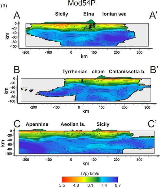
(a) Vertical sections of the VP model. The traces of the sections are shown in Fig. 1. Contours lines are at 4.5, 5, 5.5, 6, 6.5, 7, 7.7, 8 km s−1. Seismic hypocentres located less than 10 km from each section are projected. (b) Vertical sections of the Vs model. The traces of the sections are shown in Fig. 1. Contours lines are between 2.75 and 4.75 km s−1, spaced of 0.25 km s−1. Seismic hypocentres located less than 10 km from each section are projected.
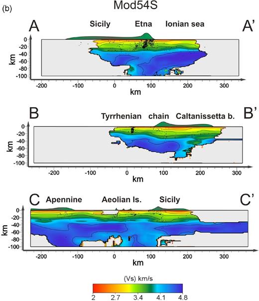
(Continued.)
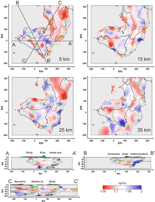
Horizontal and vertical sections of the VP/Vs model. Only the part of the model with DWSS > 200 is displayed, whereas in green the contour line DWSS = 400 is also reported. The model contours lines are at VP/Vs equal to 1.68, 1.78 and 1.88.
6.1 VP and Vs horizontal sections
In this section we discuss the main structures of the VP, Vs distributions on the horizontal planes at depth of 5, 15, 25 and 35 km (Fig. 11). Relocated earthquakes are projected onto the horizontal slices within ±5 km. Contour lines of the seismic velocities are of 0.5 km s−1 and 0.25 km s−1 with respect the mean value for the VP and Vs sections, respectively.
At depth of 5 km, both VP and Vs models show a large low velocity area (4.2 < VP < 4.7 km s−1, 2.3 < Vs < 2.8 km s−1) beneath the Fossa di Caltanissetta area (central Sicily) and Aeolian archipelago (5 < VP < 5.2 km s−1, 2.8 < Vs < 3 km s−1). High VP and Vs structures (5.5 < VP < 5.7 km s−1, 3.1 < Vs < 3.3 km s−1) are observed beneath the Hyblean Plateau. Positive anomalies of VP (5.5 < VP < 5.7 km s−1) are also observed NW of Sicily, whereas high Vs (3.25 < Vs < 3.5 km s−1) are along the NW Calabrian coastline.
At 15 km of depth, the low VP and Vs anomalies beneath the Caltanissetta basin are no longer evident. Low VP values are mostly confined in the western sector (5.2 < VP < 5.7 km s−1) whereas the Vs model exhibits low values in most of Sicily and Calabria (3.2 < Vs < 3.4 km s−1). High VP and Vs (6.2 < VP < 6.7 km s−1, 3.5 < Vs < 3.7 km s−1) characterize the southern Tyrrhenian Sea with the exception of the eastern part of the Aeolian archipelago (namely beneath Stromboli and Panarea). At this depth only the VP model is resolved in a part of the Sicily channel showing a high VP patch (6.2 < VP < 6.7 km s−1) close to the southern Sicilian coastline.
The slices at depth of 25 km clearly show low VP and Vs (6.5 < VP < 6.8 km s−1, 3.8 < Vs < 4.1 km s−1) distributions located beneath the Calabria and northern Sicily. These bodies match the position of the Apennine–Maghrebian chain. Values of VP equal to 7.1 km s−1 (Vs = 4.3 km s−1) characterize the southern Tyrrhenian region with a maximum of 7.6 km s−1 (Vs = 4.4 km s−1) in the western sector. A large low VP area, (6 < VP < 6.6 km s−1) is placed at the north of the Aeolian Arc. Weak VP velocity values (6.4 < VP < 6.6 km s−1) are also observed in the Sicily channel elongated in the N–S direction, at NE of the Pantelleria Island. In the Vs model, low seismic velocities (3.6 < Vs < 3.8 km s−1) characterize the region beneath the Hyblean Plateau.
At depth of 35 km the low velocity anomaly (7.0 < VP < 7.4 km s−1, 3.5 < Vs < 3.8 km s−1), corresponding to the Apennine–Maghrebian chain, is still visible. At this depth, low seismic velocities are also located beneath Stromboli and Panarea (VP ≈ 7.5 km s−1) with minimum values below the Marsili seamount (6.5 < VP < 7 km s−1), and in Calabria beneath the Sila area. Sicily channel is marked by P-wave velocity values greater than 8.0 km s−1 with a low VP body (VP = 7.3 km s−1) located at SE of the Hyblean Plateau. Finally, Vs model shows low values vertically elongated crossing the Hyblean Plateau (3.6 < Vs < 3.7 km s−1).
6.2 VP and Vs vertical sections
The velocity distributions of three vertical sections of mod54P and mod54S are shown in Figs 12(a) and (b). The traces relative to these sections are also reported in the Fig. 1. In the VP sections contours lines are at 4.5, 5, 5.5, 6, 6.5, 7, 7.7, 8 km s−1. The contours lines of Vs are between 2.75 and 4.75 km s−1, spaced of 0.25 km s−1. Seismic hypocentres located less than 10 km from each section are projected.
Profile AA′ shows a well-defined pattern in the depth range 20–40 km. Mantle velocity values (7.5 < VP < 8 km s−1; 3.75 < Vs < 4.00 km s−1) are present at depth of 20–25 km in the eastern and western part of the section, whereas the same values are reached at about 35 km beneath central Sicily. In the western side of the section, upwelling of the high velocities roughly corresponds to the Ionian coastline. The same section shows strong lateral heterogeneity also at depths corresponding to the upper and medium crust. In particular, the easternmost part of the section displays a shallow body with low VP (5.0 < VP < 5.5 km s−1) broadens from the coastline for 70–80 km towards W and down to 10–20 km. A high velocity anomaly (5.0 < VP < 5.5 km s−1; 2.75 < Vs < 3.00 km s−1) is evident beneath the Etna volcano at 15–20 km of depth followed by deeper low velocity zone at 25–30 km. Deep and shallow structures exhibited in mod54S (Fig. 8b) have similar patterns despite the features are much more smoothed.
Sections BB′ of the VP and Vs display lateral variations of the seismic velocities of the Sicily-Tyrrhenian domains. Typical mantle values (7.5 < VP < 8 km s−1; 3.75 < Vs < 4.0 km s−1) are present at about 15 km of depth beneath the southern Tyrrhenian Sea whereas the same velocities lie at 35–40 km beneath northern Sicily. It is worth noting that the strongest horizontal gradient characterizing the region is also marked by the clustered seismicity located in the southern Tyrrhenian Sea (i.e. the Palermo seismic sequence of 2002). The low velocity anomaly (4.5 < VP < 6.0 km s−1; 2.4 < Vs < 3.00 km s−1) located beneath the Caltanissetta basin is visible down to 5–8 km.
Section CC′ reports the seismic features of the study area, from the southern Apennine to the Sicily southern offshore. It is interesting to see how the 7.7 km s−1VP values (4.2 km s−1 of the Vs ones) range from 30–35 km beneath the Calabrian and Sicilian chains to 20–25 by the Tyrrhenian Sea. Lower velocities are imaged beneath the Aeolian archipelago especially beneath the Stromboli volcano. Low velocities bodies are always present beneath the Caltanissetta basin at shallow depths. VP section also displays an upwelling of the high velocities structures (VP = 7.7 km s−1) to 18–20 km in the Sicily channel.
6.3 VP/Vs model
In this section, we present the VP/Vs model (Fig. 13). As largely discussed in Section 4.2 the spread of VP–Vs distribution, compared to the Brocher's curve, suggests the necessity to correct the velocity models with the integration of other geophysical data, thus we will argue only on the most relevant trend observed.
At shallow depth (5–15 km) the most important feature is the difference between the easternmost sector (Calabria and eastern Tyrrhenian) with respect to the westernmost one (Sicily and western Tyrrhenian) of the study area. In the easternmost sector, low values of the VP/Vs model (1.6 < VP/Vs < 1.7) are predominant, whereas the westernmost one is marked by high values beneath Etna (VP/Vs > 1.88) and lower values (VP/Vs < 1.7) in the region between the volcano and the Caltanissetta Basin. At 15 km of depth, the Caltanissetta basin is characterized by low VP/Vs values according to the results of Sgroi et al. (2012) based on the study of the local seismicity. At greater depth (25–35 km) low VP/Vs are mostly concentrated in the Calabrian Apennine (especially beneath the Sila region), Ionian Sea and northern Sicily, whereas high values are predominant in southern Tyrrhenian and beneath the Hyblean Plateau.
In the vertical section A–A′, high VP/Vs values beneath Etna volcano at shallow depth (down to 10–15 km) are visible. An inversion of the trend occurs at depths of 30–40 km. In section B–B′, high VP/Vs values are reported beneath the Caltanissetta basin and southern Tyrrhenian down to 20–25 km of depth, and low VP/Vs are noted beneath the Sicilian-Maghrebian chain. Finally, in section C–C′ a large area with high VP/Vs in proximity of Aeolian archipelago ranges between 20 and 40 km of depth whereas low VP/Vs values are observed beneath the Apennine at the same depth range.
7 COMPARISON WITH PREVIOUS STUDIES
Several seismic velocity models have been presented to study the lithospheric structure of the southern Tyrrhenian and Sicilian area. Tomographies at larger scale (Di Stefano et al.1999, 2009; Scafidi et al.2009) imaged the whole Italian region. In such models the main patterns noted in the Sicily region can be resumed in three main observations: (i) low P-velocity anomalies in the Central-Western part of the Sicily region down to 8 km of depth; (ii) low VP beneath the Apennine chain at grater depths (20–30 km) and; (iii) strong VP horizontal gradients between Southern Tyrrhenian and Northern Sicily domains at depth between 8 and 20 km. These large-scale velocity patterns are also noted in the mod54P and further comparisons will result difficult because of the different scale of investigation of the above-mentioned models. Seismic velocity models at regional scale (Barberi et al.2004; Chiarabba et al.2008; Orecchio et al.2011) and some studies based on integrated interpretation of WARR seismic data and Bouguer anomalies (Caielli et al.2003; Chironi et al. 2000; Del Ben et al.2005) revealed the same geometries already presented by the large-scale models and improved with some more detail. Regional scale models also show the Tyrrhenian crust thinning from the Sicilian-Calabrian coastline towards offshore. Such models were obtained applying different tomographic inversion techniques. Di Stefano et al. (1999) applied the inversion tomographic code of Zhao et al. (1994), Di Stefano et al. (2009) a version modified by Di Stefano & Chiarabba (2002) whereas other authors used different versions of the Simulps code (Evans & Achauer 1993; Thurber 1993) or similar algorithms (Thurber 1993; Eberhart-Phillips & Reyners 1997). In most of the cases only absolute arrival times of the P phases to determine the velocity models and hypocentre locations were used. The horizontal resolution of these regional models was estimated of 30–40 km in the horizontal dimensions and of 8–15 km in depth. In this work, we used the tomoDD code supplemented by the WAM post-processing method. Our method allowed us to raise the resolution, the investigated volume, and the reliability of the final velocity models (Calò et al.2009, 2011, 2012). Horizontal resolution is here estimated to be between 15 and 30 km in the Tyrrhenian Sea and Sicilian areas and between 30 and 50 km in the Sicily channel, whereas the vertical one is between 2 and 10 km. Mod54P and mod54S show the main velocity structure already imaged by the previous regional models. However, in mod54P the shallow low VP anomaly is better shaped and easier distinguishable against the neighbour structures, the transition between Sicily/Calabria and the Tyrrhenian is well marked and shows a curved shape along the coastline. The higher definition is also suggested by the first imaging of tectonic lineaments, known on the surface such as Tindari-Letojanni and the limit between the Aspromonte and the Sila mountains. Finally, the new structures (e.g. the features observed beneath the Etna, Sicily Channel, southern Tyrrhenian,. etc.), described in the previous section, not identified until now in regional scale tomographies because of the lack of resolution, denote the improvement of the seismic velocity models presented in this work. The high resolution of the velocity models presented here is also confirmed by the comparison with the local tomographies performed in restricted regions of the study area. Our velocity models are consistent with the results obtained by Scarfì et al. (2007) for the Hyblean region using double-difference tomographic method and an autoadaptive mesh grid. Laigle et al. (2000), Aloisi et al. (2002), and Patané et al. (2006) investigated the volume beneath the Mount Etna using the Simulps code (Evans & Achauer 1993; Thurber 1993). All these models showed the presence of a high VP body in the easternmost part of the volcano down to a depth of 15–20 km. Analogous patterns are also observed in mod54P (Fig. 12a). Furthermore some deeper structures beneath the Etna volcano are well imaged and they were not displayed by the local scale tomography.
We thus conclude that the double-difference tomography together with the use of the post-processing WAM method allows obtaining more detailed and reliable velocity models than the previous studies. Moreover, mod54P and mod54S resulted able to recover all the velocity structures observed in the previous models, from large to small scale, by adding new insights for the study of Sicily and surrounding areas.
8 DISCUSSION AND CONCLUSIONS
We selected 3445 events recorded during 28 yr by the INGV network to calculate P- and S-waves velocity models in the Tyrrhenian-Calabrian-Sicilian region. The final velocity distributions (mod54P and mod54S) were obtained averaging the results of 54 tomographic inversions with the WAM technique. The models were previously calculated using the double-difference tomography method and three data sets. A series of assessment tests allowed assessing the reliability of the seismic velocity structures observed.
The intermediate WAM models (mod81_05, mod09_09, mod81_05_09 and mod81_09) allowed us to observe the convergence of the velocity distributions towards a well-defined seismic velocity pattern, as showed in Fig. 5, that is compatible with the whole experimental information. Slices relative to some DD models display several velocity structures that are also imaged in the intermediate models mod81_05 and mod06_09, but these are much better resulted in mod81_09 and mod81_05_09 in terms of shapes and velocity values. Koulakov et al. (2009) suggested that the effect of the noise distribution in the data on the tomographic result can be estimated by comparing tomographic results based on independent data subsets. In their case, the two subsets were built with a random selection of the errors contained in the whole data set selecting events with odd and even numbers in the earthquake list. This kind of test could be performed using performed both experimental and synthetic traveltimes. However, this approach does not take into account possible errors coming from data with different azimuthal coverage and different sampling of the structure. In our work we selected two databases and both resulted able to calculate seismic velocity models enough reliable for seismic structure reconstruction. However we also show that both models can be different in some parts, even in regions apparently sufficiently resolved by the data. This problem seems to be well managed by the WAM procedure that strongly reduces the noise effects, as smearing and artefacts, and strengthening the features presented in most of single DD models. A similar approach (tomoDD plus WAM) was already successfully applied to different data sets in various geodynamic scenarios and at different scales (Calò et al.2009, 2011, 2012; Calò & Dorbath 2013; Hofstetter et al.2012). The high reliability and resolution of our final models can be ascribed to three main reasons: (i) the selection criteria ensured a high quality of the data used. (ii) The double-difference algorithm allowed increasing the resolution of the models near the earthquake hypocentres (Zhang & Thurber 2003). This leads to a general enhancement of the whole model because of the illumination of the structures by the longer ray paths. (iii) The presence of artefacts was strongly reduced by the use of the WAM method. This post-processing provides models less dependent by the input parameters required for the tomographic inversions. The weighted staking of the models result in smoothing of the random components of the seismic velocities related to the artefacts. This also increases the coherent trend constrained by the experimental data.
The VP–Vs correlation analysis we performed has shown a manner to optimize the choice of the DWS threshold. This analysis also provides an interpretative technique, which avoids the choice of high DWS thresholds that result in a strong reduction of the investigation volume. Moreover, it gives a potential procedure that allows one to use to build VP/Vs model from VP and Vs models independently calculated. Accurate VP/Vs variations can be determined directly from the VP and Vs models if they have essentially identical quality. In cases where quantity and/or quality of the S wave arrival times are lower than P wave data, Vs model will not be resolved as well as VP, making the interpretation of VP/Vs distribution difficult (Eberhart-Phillips 1990). On the other hand, VP/Vs models can be determined by the inversion of S–P time differences (Walck 1988; Thurber 1993). This is possible by assuming that the ray paths of P- and S-waves are identical. However this last approach implies two potential problems: (i) In the case of complex 3-D structure, some P- and S-ray paths may differ significantly and thus the results may be biased; (ii) the Vs structure cannot be inferred reliably from VP and VP/Vs values (Wagner et al.2005). Thus the VP–Vs analysis performed here could offer a guideline for selecting reliable part of the VP/Vs model directly calculated by the VP and Vs distributions.
The velocity models obtained in this study give a detailed view of the lithospheric structures in a part of the southern Italy. The Moho discontinuity is well imaged in the whole area allowing the description in detail of the oceanic-continental transition in the southern Tyrrhenian Sea and partially in the Ionian Sea (the capability to reproduce strong vertical gradient was assessed throughout synthetic tests).
Large low velocity anomalies mark the regions of the Marsili seamount and the western part of the Aeolian archipelago. Calò et al. (2009, 2012) have already showed this pattern by applying the WAM procedure to shallow and deep events related to the subduction of the Ionian lithosphere. However, Calò et al. (2012) focusing on the study of the deep structures, showed the shallower ones (20–40 km) with a minor resolution. Here, the higher resolution of these features provides new insights on the size of the main seismic anomalies in southern Tyrrhenian at shallower depth (less than 40 km). Nevertheless, in both models this pattern can be easily associated to the huge volcanic activity affecting the eastern Tyrrhenian sector. D'Alessandro et al. (2009), using signals collected by an ocean Bottom Seismometer installed at the top of the volcano, reported the presence of an intense microseismicity around the station suggesting a huge hydrothermal and volcanic activity in the area.
The basement of the Maghrebian chain, notable down to a depth of 35–40 km, shows continuity with the Apennine chain in the E–W direction at least beneath the Palermo region. Depth estimation of the Moho discontinuity is in agreement with the results of Sgroi et al. (2012). According to the results of Accaino et al. (2011) and of Dezes & Ziegler (2002), the Sicilian crust deepens at a low-angle northward, from 20–28 km beneath Sicily channel to 35–40 km beneath the Sicilian-Maghrebian mountains domain (Figs 7 and 8; profile B and C). A different velocity pattern is observed for the first time between eastern and western part of the Sicilian-Maghrebian chain in the first 20–25 km of depth (Fig. 8a; section A–A′).
Low VP, Vs and VP/Vs characterize the Caltanissetta region suggesting that it does not represent a simple monocline fore-arc basin but rather a huge concave region subjected to tectonic compression. Hyblean Plateau, being a monocline dipping towards N–W, supports this tectonic scenario and justifies the presence of deep low Vs and high VP/Vs because of the local distension occurred before the bending of the African-Sicilian lithosphere beneath the Marghrebian chain.
An interesting aspect is the pattern observed in section A–A′ beneath Etna volcano. The high VP velocity anomaly (5.0 < VP < 5.5 km s−1; 2.75 < Vs < 3.00 km s−1) and high VP/Vs down to 15–20 km of depth was already imaged by several authors and interpreted as the expression of the upwelling of deep mantle material (Laigle et al.2000; Aloisi et al.2002; Patané et al. 2006). In our models, similar P-wave seismic velocities are observed down to 25–35 km suggesting that the root of this upwelling could start at greater depth where the crust-mantle transition is expected. At this depth the lower values of VP/Vs should be because of the fact that the higher pressures do not allow melting of the upwelling mantle. These observations are compatible with the geodynamic context of this part of Sicily and support the theory of existence of a local distension zone facilitating a preferential magma ascent feeding the volcanic activity.
Mod45P displays Sicily channel as mostly characterized by high seismic velocities at depths greater than 30 km (VP > 8 km s−1). Although in this region the lower resolution of the seismic velocity model does not allow observing the smaller features (the resolution in this part of the model is estimated of 40–50 km), some low VP bodies are imaged at crustal depths (15–25 km) between Pantelleria and the Sicily coastline, in the region involved in some volcanic activity almost two centuries ago (i.e. the Ferdinandea volcanic island eruption).
In conclusion, the seismic data analysis performed in this study allowed us to build highly resolved and reliable seismic VP and Vs velocity models of the Tyrrhenian-Sicilian region. We showed an assessment procedure to evaluate the reliability of the features observed in the seismic velocity models. Both VP and Vs distributions allowed identifying the Moho depth as well as many crustal structures related to the complex geodynamic pattern of the region.
Hence, these models contribute to providing a more complete picture of the southern Italy lithosphere and represent a basic knowledge useful for further investigations.
During this work L. Parisi was supported by the Erasmus Placement (European Parliament n. 1720/2006/CE) and ‘Perfezionamento All'Estero’ grants funded by the Università degli Studi di Palermo. We are grateful to the INGV crew who manage the seismic network and data. In particular we thank Franco Mele for his support to satisfy our specific request. Some figures were generated using the generic mapping tools (GMT, Wessel & Smith 1995). Finally, we very sincerely thank Andrea Morelli and the two anonymous reviewers who helped improve the quality of the manuscript.
REFERENCES
APPENDIX A
Mean values of the parameters used to calculate 54 DD inversions selected for the construction of the final WAMs (mod54P and mod54S). Each line contains an identification number (ID), the data set used (Data set), the initial velocity model (Mod), the maximum, mean, and minimum node spacing of the inversion grid in the horizontal and vertical directions (Spacing H-V), the clockwise rotation angle with respect to the North direction (ROT), and the weights of the absolute (Abs) and differential (Diff) data adopted for each loop of iterations. The weighting scheme of the data also reports the number of the loops that varied between 3 and 8. In each loop, the number of iterations varied between 1 and 4. For each velocity model, the number of iterations ranges between 7 and 11. The weighting scheme is the same both for the P- and S-traveltime data sets.
| ID | Data set | Mod | Spacing H-V (km) | ROT (°) | Abs weights | Diff weights | ||
|---|---|---|---|---|---|---|---|---|
| Min | Mean | Max | ||||||
| N01 | 81_05 | M1 | 15–2 | 31.4–6.6 | 50–10 | 0 | 1–0.1–1.5–0.1–10–1 | 1–1–1–0.1–1–1 |
| N02 | 81_05 | M1 | 15–2 | 31.4–6.6 | 50–10 | 30 | 1–0.1–1.5–0.1–10–1 | 1–1–1–0.1–1–1 |
| N03 | 81_05 | M1 | 15–2 | 31.4–6.6 | 50–10 | 60 | 1–0.1–1.5–0.1–10–1 | 1–1–1–0.1–1–1 |
| N04 | 81_05 | M1 | 15–2 | 31.4–6.6 | 50–10 | 90 | 1–0.1–1.5–0.1–10–1 | 1–1–1–0.1–1–1 |
| N05 | 81_05 | M1 | 15–2 | 31.4–6.6 | 50–10 | −30 | 1–0.1–1.5–0.1–10–1 | 1–1–1–0.1–1–1 |
| N06 | 81_05 | M1 | 15–2 | 31.4–6.6 | 50–10 | −60 | 1–0.1–1.5–0.1–10–1 | 1–1–1–0.1–1–1 |
| N07 | 81_05 | M2 | 20–2 | 34.4–7.4 | 50–20 | 0 | 1–10–1 | 10–10–1 |
| N08 | 81_05 | M1 | 15–2 | 30.9–6.5 | 50–20 | 0 | 1–0.1–1.5–0.1–10–1 | 1–1–1–0.1–1–1 |
| N09 | 81_05 | M1 | 5–2 | 29–6 | 40–10 | 0 | 1–0.1–1.5–0.1–10–1 | 1–1–1–0.1–1–1 |
| N10 | 81_05 | M1 | 30–2 | 30–6 | 30–10 | −30 | 1–0.1–1.5–0.1–10–1 | 1–1–1–0.1–1–1 |
| N11 | 81_05 | M1 | 30–2 | 30–6 | 30–10 | −50 | 1–0.1–1.5–0.1–10–1 | 1–1–1–0.1–1–1 |
| N12 | 81_05 | M1 | 20–2 | 34.4–6 | 50–10 | 0 | 1–10–1 | 10–10–1 |
| N13 | 81_05 | M1 | 30–2 | 30–6 | 30–10 | −70 | 1–0.1–1.5–0.1–10–1 | 1–1–1–0.1–1–1 |
| N14 | 81_05 | M1 | 30–2 | 30–6 | 30–10 | 0 | 1–0.1–1.5–0.1–10–1 | 1–1–1–0.1–1–1 |
| N15 | 81_05 | M1 | 30–2 | 30–6 | 30–10 | 0 | 1–0.1–1.5–0.1–10–1 | 1–1–1–0.1–1–1 |
| N16 | 81_05 | M1 | 30–2 | 30–6 | 30–10 | 30 | 1–0.1–1.5–0.1–10–1 | 1–1–1–0.1–1–1 |
| N17 | 81_05 | M1 | 30–2 | 30–6 | 30–10 | 50 | 1–0.1–1.5–0.1–10–1 | 1–1–1–0.1–1–1 |
| N18 | 81_05 | M1 | 30–2 | 30–6 | 30–10 | 70 | 1–0.1–1.5–0.1–10–1 | 1–1–1–0.1–1–1 |
| N19 | 81_05 | M1 | 30–2 | 30–6 | 30–10 | 90 | 1–0.1–1.5–0.1–10–1 | 1–1–1–0.1–1–1 |
| N20 | 06_09 | M2 | 20–2 | 35.1–7.4 | 50–20 | −15 | 1–1–1–1–10 | 0.1–0.1–1–1–10 |
| N21 | 06_09 | M2 | 20–2 | 35.1–7.4 | 50–20 | −30 | 1–1–1–1–10 | 0.1–0.1–1–1–10 |
| N22 | 06_09 | M2 | 20–2 | 35.1–7.4 | 50–20 | −45 | 1–1–1–1–10 | 0.1–0.1–1–1–10 |
| N23 | 06_09 | M2 | 20–2 | 35.1–7.4 | 50–20 | −60 | 1–1–1–1–10 | 0.1–0.1–1–1–10 |
| N24 | 06_09 | M2 | 20–2 | 35.1–7.4 | 50–20 | −90 | 1–1–1–1–10 | 0.1–0.1–1–1–10 |
| N25 | 06_09 | M1 | 20–2 | 34.4–6 | 50–10 | 0 | 1–10–1 | 10–10–1 |
| N26 | 06_09 | M2 | 20–2 | 35.1–7.4 | 50–20 | 0 | 1–1–1–1–10 | 0.1–0.1–1–1–10 |
| N27 | 06_09 | M2 | 20–2 | 35.1–7.4 | 50–20 | 0 | 1–1–1–1–10 | 0.1–0.1–1–1–10 |
| N28 | 06_09 | M2 | 20–2 | 35.1–7.4 | 50–20 | 30 | 1–1–1–1–10 | 0.1–0.1–1–1–10 |
| N29 | 06_09 | M2 | 20–2 | 35.1–7.4 | 50–20 | 90 | 1–1–1–1–10 | 0.1–0.1–1–1–10 |
| N30 | 06_09 | M2 | 20–2 | 35.1–7.4 | 50–20 | 15 | 1–1–1–1–10 | 0.1–0.1–1–1–10 |
| N31 | 06_09 | M2 | 20–2 | 35–7.5 | 50–15 | 0 | 1–1–1–1–10 | 0.1–0.1–1–1–10 |
| N32 | 06_09 | M2 | 20–2 | 35–7.3 | 50–17 | 0 | 1–1–1–1–10 | 0.1–0.1–1–1–10 |
| N33 | 06_09 | M2 | 20–2 | 35.1–7.4 | 50–20 | 0 | 5–8–2–5–10 | 0.5–0.8–2–5–10 |
| N34 | 06_09 | M2 | 20–2 | 35.1–7.4 | 50–20 | 0 | 10–1–1–1–1 | 1–1–1–1–1 |
| N35 | 06_09 | M2 | 20–2 | 35.1–7.4 | 50–20 | 0 | 10–10–1–1–1 | 1–1–1–1–1 |
| N36 | 06_09 | M2 | 15–2 | 31.6–7.4 | 50–20 | 0 | 1–1–1–1–10 | 0.1–0.1–1–1–10 |
| N37 | 06_09 | M2 | 15–2 | 31.6–7.4 | 50–20 | 0 | 10–10–5–8–10 | 1–1–5–8–10 |
| N38 | 06_09 | M2 | 20–2 | 35.1–7.4 | 50–20 | 0 | 1–1–1–1–1–1–10–10 | 10–10–1–1–1–1–1–1 |
| N39 | 06_09 | M2 | 20–2 | 34.4–7.4 | 50–20 | 0 | 1–10–1 | 10–10–1 |
| N40 | 81_09 | M3 | 18–4 | 34.7–7.4 | 55–20 | 30 | 0.1–1–8–1 | 10–10–8–1 |
| N41 | 81_09 | M3 | 18–4 | 34.7–7.4 | 55–20 | 30 | 0.1–1–8–1 | 10–10–8–1 |
| N42 | 81_09 | M3 | 18–2 | 34.7–7.4 | 55–20 | 0 | 0.1–1–8–1 | 10–10–8–1 |
| N43 | 81_09 | M2 | 20–4 | 34.6–6.4 | 45–15 | 0 | 0.1–1–10–1 | 10–10–10–1 |
| N44 | 81_09 | M2 | 20–4 | 34–7.4 | 50–27 | 0 | 0.1–1–10–1 | 10–10–10–1 |
| N45 | 81_09 | M2 | 15–2 | 36–7.4 | 70–20 | 0 | 0.1–1–8–1 | 10–10–8–1 |
| N46 | 81_09 | M2 | 20–2 | 24.2–8 | 50–20 | 30 | 0.1–1–10–1 | 10–10–10–1 |
| N47 | 81_09 | M2 | 10–4 | 34.1–6.2 | 50–12 | 0 | 0.1–1–10–1 | 10–10–10–1 |
| N48 | 81_09 | M2 | 15–2 | 34.4–6.8 | 70–20 | 70 | 0.1–1–10–1 | 10–10–10–1 |
| N49 | 81_09 | M2 | 10–4 | 34.1–6.2 | 50–12 | 20 | 0.1–1–10–1 | 10–10–10–1 |
| N50 | 81_09 | M2 | 10–4 | 34.1–6.2 | 50–12 | −20 | 0.1–1–10–1 | 10–10–10–1 |
| N51 | 81_09 | M2 | 20–2 | 24.2–8 | 50–20 | 0 | 0.1–1–10–1 | 10–10–10–1 |
| N52 | 81_09 | M2 | 20–2 | 24.2–8 | 50–20 | −45 | 1–0.1–1–10–1 | 1–10–10–10–1 |
| N53 | 81_09 | M2 | 15–2 | 34.4–6.8 | 70–20 | 50 | 0.1–1–10–1 | 10–10–10–1 |
| N54 | 81_09 | M2 | 15–2 | 34.4–6.8 | 70–20 | −70 | 0.1–1–10–1 | 10–10–10–1 |
APPENDIX B
Horizontal and vertical sections of the VP and Vs WSTD are reported in Figs B1 and B2, respectively. The WSTD are determined using the 54 velocity models selected to build the final WAMs (mod54P and mod54S), and calculated giving to each estimate the same weight assigned to the corresponding velocity value.
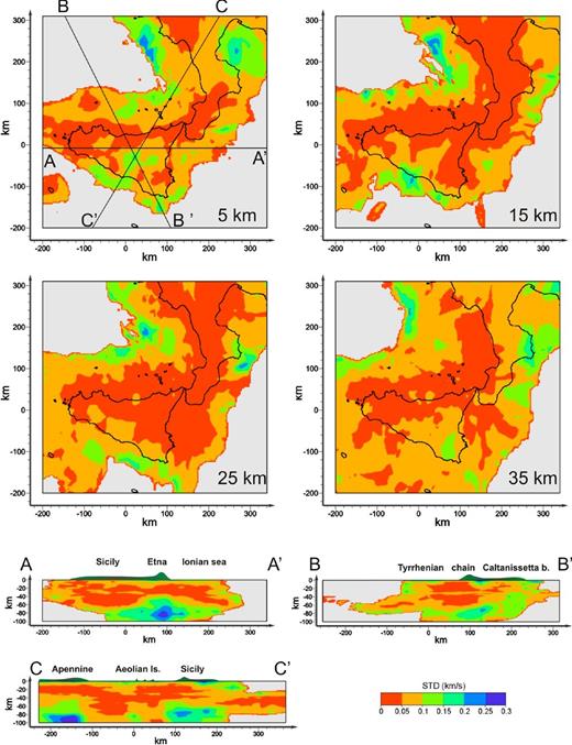
Horizontal and vertical sections showing the WAM standard deviation for the mod54P (standard deviation of the 54 VP velocity models).
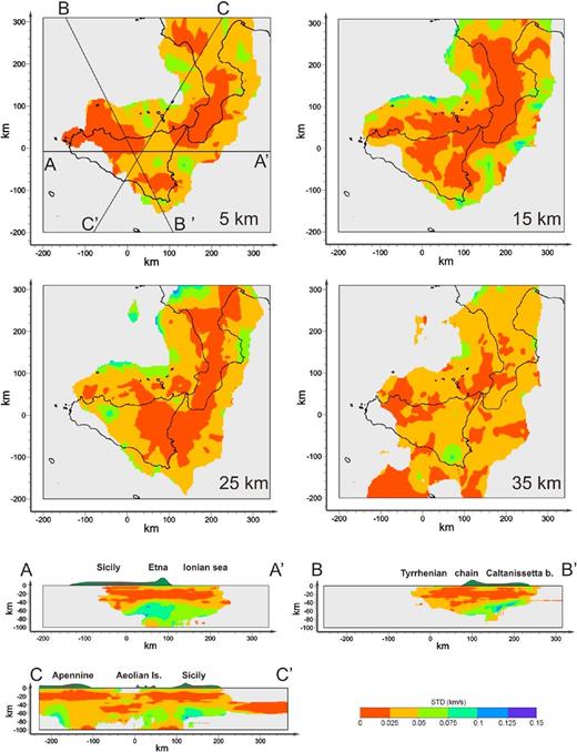
Horizontal and vertical sections showing the WAM standard deviation for the mod54S (standard deviation of the 54 Vs velocity models).
The WSTD provides a distribution of the fraction of the total uncertainty produced by the arbitrariness of the input parameters in models obtained with a single inversion. Assessment tests have shown that the WSTD decreases as the WAM order (number of single inversion considered) increases (Calò 2009). Therefore, portions of the model marked by a large value of WSTD are consequence of a strong dependence of the models on the input parameters, suggesting a poor constraining of the experimental data. This fact highlights a lower reliability of those parts of the velocity model. Some synthetic tests (Calò 2009), have shown that the WSTD is well correlated with some restoration indexes, supporting the idea that it can be used as reliability estimator. For example, in section C–C′ a high spatial coherence between a maximum of the WSTD and a low VP anomaly is observed beneath Sicily at a depth of 80 km. Seismic sources in this region are shallower than the position of the VP anomaly and only the longest and deepest ray paths sample this region. Hence, in this case we cannot exclude that the velocity anomaly is biased by the inversion procedure and though it is consistent with some of the data used, probably it is distorted by smearing effects.
However, the WSTD values of the mod54P and mod54S are smaller than 0.15 km s−1 for most of the investigated volume and the absence of strong spatial correlation between the highest WSTD and velocity anomalies ensures a high reliability of most of the anomalies, even considering a confidence interval of width 2σ (∼95 per cent confidence level).
