


Abstract
We present a 1-D velocity model of the Earth's crust in Campania–Lucania region obtained by solving the coupled hypocentre–velocity inverse problem for 1312 local earthquakes recorded at a dense regional network. The model is constructed using the VELEST program, which calculates 1-D ‘minimum’ velocity model from body wave traveltimes, together with station corrections, which account for deviations from the simple 1-D structure.
The spatial distribution of station corrections correlates with the P-wave velocity variations of a preliminary 3-D crustal velocity model that has been obtained from the tomographic inversion of the same data set of P traveltimes. We found that station corrections reflect not only inhomogeneous near-surface structures, but also larger-scale geological features associated to the transition between carbonate platform outcrops at Southwest and Miocene sedimentary basins at Northeast.
We observe a significant trade-off between epicentral locations and station corrections, related to the existence of a thick low-velocity layer to the NE. This effect is taken into account and minimized by re-computing station corrections, fixing the position of a subset of well-determined hypocentres, located in the 3-D tomographic model.
1 INTRODUCTION
The analysis of regional seismicity to identify and geometrically characterize active fault structures and estimate the present tectonic regime requires an accurate determination of the spatial distribution of the earthquakes. The quality of absolute event locations is controlled by several factors, including network geometry, number of available phases, arrival-time reading accuracy and information about the crustal structure (Pavlis 1986; Gomberg et al.1990).
The knowledge of a realistic velocity structure is necessary to prevent artefacts in the location of hypocentres: inappropriate choice of the velocity model can lead to significant distortions and bias in the hypocentre positions, even when using double-difference methods (Michelini & Lomax 2004).
Parametrizing the Earth crust structure as a layered medium is generally appropriate, since the elastic proprieties of the Earth mainly change with depth due to sedimentation, compaction and thermal processes. The importance of finding a reliable, 1-D reference velocity model has been emphasized in many works (e.g. Crosson 1976; Thurber 1983; Kissling et al.1995). 1-D velocity models are routinely used in seismic network operations and in seismological studies to estimate earthquake location, focal mechanisms and other seismic source parameters. Layered velocity models are also required by several methods for the calculation of synthetic Green's function, like the widely used discrete wavenumber approach (Bouchon 2003). Finally, 3-D tomographic models are often obtained as perturbations of a 1-D reference model. Tomographic results and resolution estimates strongly depend on the choice of the initial model: inadequate reference models may in fact severely distort the tomographic images or introduce artefacts that lead to misinterpretations of the results (Kissling et al.1995).
In regions with strong lateral variations and irregular topographic surface, significant errors or systematic shifts in earthquake locations can be introduced by the use of simplified 1-D velocity parametrization. In some cases, the complexity of geological structures can be only represented by 3-D velocity models. In many cases, however, one can (partially) account for the velocity lateral variations by including station and/or source terms in the location procedure (Douglas 1967; Pujol 1988; Shearer 1997) or path-dependent calibrations (Zhan et al.2011).
In this paper we determine a 1-D velocity model for earthquake location for the Campania–Lucania region (Southern Italy), a complex area with geological and geophysical evidence of significant lateral variations of the elastic properties of the medium, associated with the Apenninic fold and thrust-belt geological formation.
The Campania–Lucania region is one of the most active seismic zones of the Apenninic chain: large destructive earthquakes occurred both in historical and recent times (Fig. 1a). The most recent major event (Irpinia earthquake, Ms 6.9) occurred on 1980 November 23 and was characterized by a complex normal fault mechanism (e.g. Westaway & Jackson 1987; Bernard & Zollo 1989; Pantosti & Valensise 1990; Amato & Selvaggi 1993). Since then, a normal faulting mechanism earthquake (ML = 4.9) occurred within the epicentral area of the 1980 earthquake on 1996 April 3 (Cocco et al.1999). Two moderate magnitude seismic sequences occurred in 1990 and 1991 (ML = 5.2 and ML = 4.7 for the two main shocks) in the Potenza region, located about 40 km SE of the 1980 Irpinia aftershock area. These sequences were characterized by dextral strike-slip faulting mechanisms with E–W orientation (Ekstrom 1994; Di Luccio et al.2005; Boncio et al.2007).

At present the area is characterized by several seismic swarms (Stabile et al.2012) and significant low-magnitude (ML < 3.5) background seismicity that delineates both NW–SE–striking structures along the Apenninic chain (Irpinia fault system) and a nearby approximately E-W oriented, strike-slip fault, transversely cutting the chain (De Matteis et al.2012).
Many 1-D velocity models available in the literature have been used for the study region at different spatial scales: for the analysis of the 1997–2002 Italian Seismic Catalogue (Chiarabba et al.2005); for the study of the recent seismicity of the Lucania Apennines and Bradano foredeep (Maggi et al.2009); for the characterization of the aftershocks of the 1980 Irpinia earthquake (Bernard & Zollo 1989; Amato & Selvaggi 1993; De Matteis et al.2010). These velocity models have significant differences in P-wave velocity values, and in number and depth of interfaces. This is likely due to the different tools and data used in each study, as well as to the true complexity of the propagation medium.
Starting from 2005, with the deployment of the dense, wide-dynamic range, Irpinia Seismic Network (ISNet; Weber et al.2007), the capability of detecting and accurately locating small magnitude events (ML <3.5) in the Campania–Lucania region has greatly increased. Automatic detection, complemented by manual revision and integration of the event catalogue, has provided a new, large data set of high-quality phase readings that we used for determining a new reference 1-D model of the region.
In this work we present this new model, and we illustrate the approach used to determine a robust and reliable 1-D reference structure for the area that takes into account for the actual complexity of the propagation medium through well-defined traveltime station corrections. The data set consists of 1312 events occurred in the period 2005 August–2011 April and recorded at 42 seismic stations. The 1-D velocity model and the associated station corrections have been constructed through a three-step procedure:
A P-wave ‘Minimum 1-D velocity model’ is calculated following the approach of Kissling et al. (1995), by joint inversion of layered velocity model, station corrections and hypocentre locations.
Starting from the 1-D model, a preliminary 3-D crustal velocity model is computed, using a linearized and iterative tomographic algorithm (Latorre et al.2004; Vanorio et al.2005). This model is used to study the relation between station corrections and lateral velocity variations and to identify a well-constrained event to use for refined station correction calculation in step (3).
Refined 1-D station corrections are calculated by fixing the location of well-constrained events, obtained in step (2).
2 GEOLOGICAL AND GEOPHYSICAL SETTING OF THE INVESTIGATED AREA
The Campania–Lucania region is located in the axial portion of the Southern Appennines an Adriatic-verging fold and thrust belt, orogenically transported over the flexured southwestern margin of the Apulian foreland, in subduction towards the SW, which developed since the late Cretaceous till the Quaternary (Patacca & Scandone 1989). The belt is associated with the Tyrrhenian backarc basin to the West and with the Bradano foredeep to the East (Fig. 1a). During the middle Miocene-upper Pliocene, several compressional tectonic phases, associated with the collision between the African and European margin, determined thrusting and piling of different units towards stable domains of the Apulo-Adriatic foreland (Apulian Carbonate Platform, ACP). From late Tortonian to Quaternary, the whole system rapidly migrated to the East as a consequence of the ‘eastward’ retreat of the sinking foreland lithosphere (Malinverno & Ryan 1986; Patacca & Scandone 1989; Patacca et al.1990).
The present-day structural complexity of the chain is due to the different palaeogeographic domains involved in the Southern Appenine thrust belt building (the carbonate platforms underwent brittle deformation whereas the basinal domains underwent a ductile deformation) but also to several deformational episodes that led to the formation of the chain. Since the lower-middle Pleistocene, the axial zone of the chain is in an extensional NE–SW regime. This regime is still active, as shown by the analysis of surface geological indicators, breakout and seismic data (Pantosti & Valensise 1990; Frepoli & Amato 2000; Montone et al.2004; Pasquale et al.2009; DISS Working Group 2010; De Matteis et al.2012), and it is responsible for the present-day seismicity in Southern Apennines.
The structural setting of the Campania–Lucania region has been defined by several geological and geophysical studies, including: tomographic images (Amato & Selvaggi 1993; Chiarabba & Amato 1994; De Matteis et al.2010), analysis and joint interpretation of gravity data, seismic reflection lines and subsurface information from many deep wells (Improta et al.2003), seismic reflection analysis and investigations for hydrocarbon exploration (Mostardini & Merlini 1986; Patacca & Scandone 1989, 2001; Casero et al.1991; Roure et al.1991; Menardi & Rea 2000; Scrocca et al.2005—Fig. 1b).
The inferred models show important lateral variations of the properties of the medium mainly along a direction perpendicular to Apenninic belt in the upper crust. This is consistent with the presence of a Platform domain to the SW and with the basinal deposits to the NE. In addition, important lithological variations are evident along the chain, the most relevant being an abrupt deepening of the ACP in the southeastern part of the investigated region (Improta et al.2003). The velocity structure in the upper crust is strongly influenced by the geometry of the ACP, whose structural lows and highs give rise to pronounced low- and high-velocity anomalies.
The results of sonic logs, wide-angle refraction data interpretation and velocity analysis performed on seismic reflection data (from Improta et al.2003) allowed for the studied area to associate a P-wave velocity value range to each tectono-stratigraphic unit.
The ACP consists of a 7- to 8-km-thick Meso–Cenozoic carbonate sequence, which overlies Permotriassic clastic deposits (Verrucano Fm., Roure et al.1991), with P-wave rock velocities ranging between 6.0 and 6.5 km s−1. Plio–Pleistocene terrigenous deposits stratigraphically cover the flexed ACP in the eastern margin of the Bradano Trough (Casnadei 1988). Towards the west, the external zone of the belt, the ACP progressively dips below the rootless nappes and it is in turn involved in the folds and thrusts of the thrust belt (Fig. 1b).
The thrust sheet stacks overlying the ACP are derived from the deformation of the following main palaeogeographic domains (Fig. 1a; Patacca et al.1992):
Successions with shallow-water, basinal and shelf-margin facies, ranging in age from middle Triassic to Miocene (‘Lagonegro Basin units’, LB), located between the ACP and the Western Carbonate Platforms (WCPs). LB units can be differentiated in two complementary lithostratigraphic sequences: (i) a Triassic–Lower Cretaceous sequence (with P-wave velocity ranging from 4.4 to 6.2 km s−1); (ii) Upper Cretaceous–Lower Miocene plastic succession (with P-wave velocity ranging from 3.5 to 4.4 km s−1).
The WCP successions (with P-wave velocity ranging from 5.3 to 6.0 km s−1), overthrust on the Lagonegro units. They consist of Mesozoic and Palaeogene carbonate sequences followed by Upper Miocene siliciclastic flysch deposits, the latter accumulated above the WCP during its foredeep phase.
Jurassic–Cretaceous to Miocene deep-water successions (ophiolite or ‘internal’ units and associated siliciclastic wedges), outcropping on the Tyrrhenian belt and the Calabria–Lucania boundary, overthrust on the Apenninic platform units (Sannio and Sicilide Complexes). They consist of variegated clays, arenaceous turbidites and carbonate sediments that appear often as chaotic tectonic mélanges (with P-wave velocity ranging from 2.8 to 5.2 km s−1). They have been incorporated in the thrust belt before the opening of the Tyrrhenian Basin and correspond to the geometrically highest structural units in the Southern Apennines.
Syntectonic terrigenous sequences (with P-wave velocity ranging from 2.0 to 2.4 km s−1) unconformably cover the thrust sheet stacks and represent the infill of satellite basins of Late Tortonian to Early Pleistocene age (Patacca & Scandone 2001).
3 SEISMIC NETWORKS AND DATA COLLECTION
Since 2005, the seismic activity in the Campania–Lucania region is monitored by ISNet (Irpinia Seismic Network), a permanent seismic network operated by the research consortium AMRA (Analysis and Monitoring of Environmental Risk), consisting of 26 stations covering an area of 100 km × 70 km, with average interstation distance from 10 to 30 km. ISNet is equipped with collocated tri-axial strong-motion accelerometers and three-components short-period or broad-band seismometers, allowing for high dynamic range (Weber et al.2007). The data set collected by ISNet is extended and integrated by the inclusion of the closest stations of the Italian Seismic Network, managed by INGV (Istituto Nazionale di Geofisica e Vulcanologia), allowing for better quality in the determination of the hypocentral parameters.
The data set used in this study consists of 17 202 traces recorded by 42 ISNet and INGV stations from 1312 small-magnitude earthquakes, with local magnitude ranging between 0.1 and 3.2 (Fig. 2b), occurred from 2005 August to 2011 April. To obtain a high-quality data set, we manually picked the first P- and S-wave arrival times of earthquakes recorded by at least four stations. A weighting factor was assigned to the readings of the first P- and S-wave arrival times according to the estimated uncertainties (decreasing weighting factors were associated to uncertainties <0.05 s, 0.05–0.10 s, 0.10–0.20 s, 0.20–0.50 s and >0.50 s).
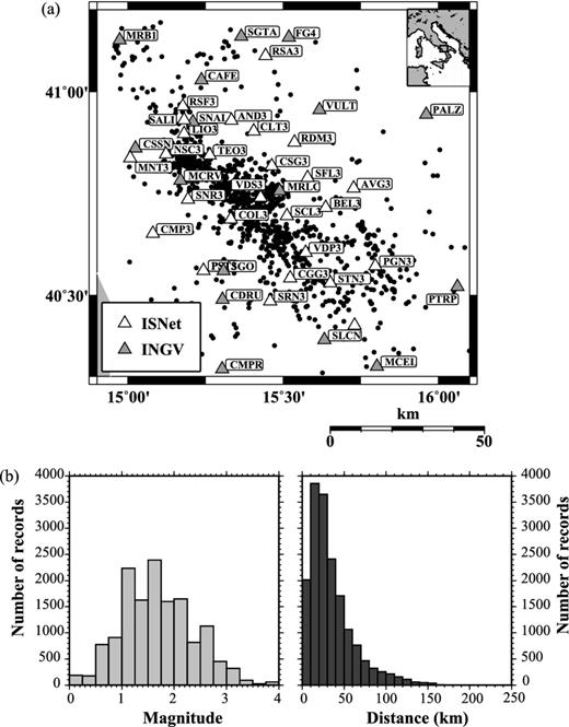
(a) Epicentral map showing routine locations of the studied earthquakes. Triangles are INGV (in grey) and ISNet (white) stations. (b) Histograms of number of records as function of local magnitude and epicentral distance.
A first evaluation of picking consistency has been performed by analysing the ‘modified Wadati diagram’ (Chatelain 1978), which also provides an estimate of the average Vp/Vs ratio. In this diagram, we considered for each event, and for each pair of station (i, j), the difference between P-phase (TPi − TPj, x-axis) and S-phase (TSi − TSj, y-axis) arrival times; this representation does not depend on the earthquake origin time. The data are well distributed around a linear trend and the least-square best-fit line provides a slope, equal to the Vp/Vs ratio, of 1.885 with an rms of 0.003, and linear correlation coefficient (R2) of 0.98 (Fig. 3). Arrival times that departed significantly from this trend were considered as outliers and therefore identified and removed from the data set.
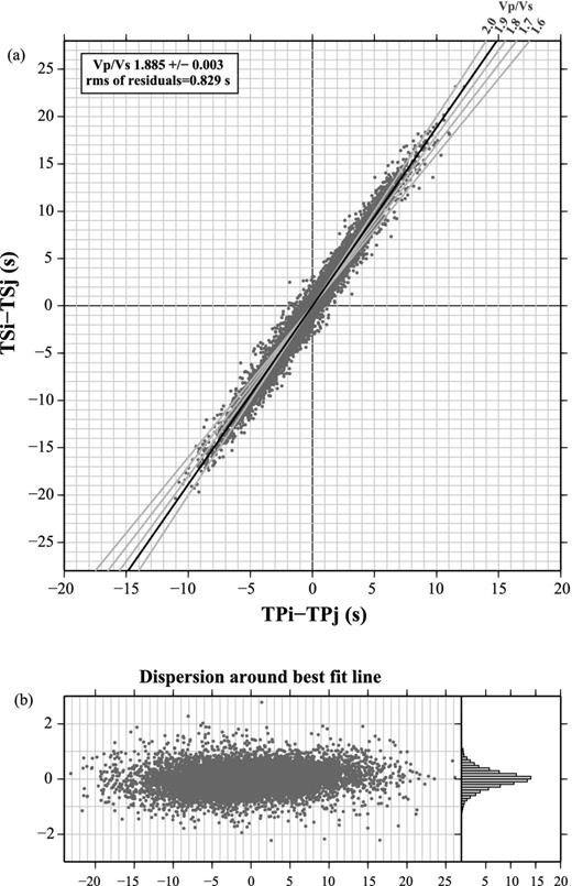
(a) ‘Modified Wadati diagram’ showing for each event, and for each pair of station (i, j), the difference between P-phase (TPi − TPj, x-axis) and S-phase (TSi − TSj, y-axis) arrival times. In black is the best-fit line (which provides an estimate of an average Vp/Vs ratio of 1.885 ± 0.003), in grey are the theoretical lines for several values of Vp/Vs ratio. (b) Dispersion of the points around the best-fit line.
The picking quality has been further assessed by performing a preliminary location in a homogeneous medium (Vp = 5.5 km s−1; Vp/Vs = 1.88) using the NonLinLoc code (Lomax et al.2000) and looking, for each station, for outliers on the histogram of residuals (difference between the observed and the calculated traveltime). We performed a selection removing picks significantly outside the distribution of residuals (>1 s), and the final data set consists of 11 612 P- and 6718 S-arrival time readings.
4 1-D P-WAVE VELOCITY MODEL
Seismic wave traveltime is a non-linear function of the hypocentral parameters and of the seismic velocities sampled along the ray path between the hypocentre and the station. The bias between the hypocentral parameters and seismic velocity is known as the ‘coupled hypocentre–velocity model problem’ (Crosson 1976; Kissling 1988; Thurber 1992). In a standard location procedure, the velocity parameters are maintained fixed to a priori values and the observed traveltime residuals are minimized by perturbing the four hypocentral parameters (origin time, epicentre coordinates and depth). Precise hypocentre locations demand the simultaneous solution of both velocity and hypocentral parameters.
In order to determine the best P-wave 1-D velocity model of the study area we used the VELEST code developed by Kissling et al. (1995). The non-linear problem is linearized and the solution is obtained iteratively, each iteration consisting in solving both the complete forward problem and the complete inverse problem at once. The inverse problem is solved by inversion of the damped least-square matrix of traveltime partial derivatives. To account for velocity lateral heterogeneities in the subsurface, station corrections are included in the ‘minimum 1-D velocity model’ inversion. For a more detailed description of VELEST methodology the reader is referred to Kissling (1995).
VELEST solves for the S- and the P-wave velocity model independently or jointly. It is suitable for cases in which the ratio Np/Ns (Np and Ns being the number of P and S time readings, respectively) is high and the uncertainties on the S-wave readings are comparable with P uncertainties. We restricted this study to the Vp model determination since the amount and the quality of S-wave arrival times were not sufficiently high to obtain a reliable and accurate Vs model, and we chose to find the best average Vp/Vs ratio considering the P-wave velocity models as the reference models.
In the inversion process we considered only the events with the following features: at least five P-arrival time readings, azimuthal gap smaller than 200°, a maximum location error (both horizontal and vertical) of 10 km, and maximum rms of 0.5 s. This refined data set is composed of 4620 first P arrival time readings, corresponding to 390 localized events.
A critical factor for the linearized inverse problem, already stressed by several authors (Kissling 1988; Thurber 1992; Kissling et al.1995), is the importance of the initial velocity model that affects the whole process of inversion. Here we tackle this problem by exploring 11 different 1-D initial Vp models, five of which are taken from literature and the remaining six being simple homogeneous or gradient models.
Several authors produced 1-D velocity models for the Irpinia region from either local-scale or large-scale studies of the seismicity. In particular (Fig. 4a), the model of Chiarabba et al. (2005) is used for earthquake location of the Italian seismicity catalogue from 1997 to 2002; the model by Maggi et al. (2009) is derived from an analysis of the recent instrumental seismicity of the Lucanian Apennines and Bradano foredeep; the models from Amato & Selvaggi (1993), De Matteis et al. (2010) and Bernard & Zollo (1989) are computed considering the aftershocks of the 1980 Irpinia earthquake. These models, displayed in Fig. 4(a), show a very broad range of P-wave velocities in the top few first kilometres that decrease with depth reflecting the sharp lateral variation of velocity in the upper first 15 km of the crust. Also, the number of interfaces and their depth are very different from one model to another: this probably reflects the actual complexity of the area as well as the different assumptions, tools and data used in each study.
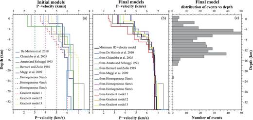
(a) The 11 1-D P-wave velocity structures used as initial models for the VELEST inversion procedure. Five of them (solid lines) are from literature; the remaining six are simple homogeneous or gradient models. (b) Final velocity models obtained from the VELEST inversion procedure starting from each of the different initial models shown in panel (a). The ‘minimum’ 1-D P-wave velocity model, obtained by a last inversion step, starting from an average of the 11 final models, is represented with a black thick line. (c) Histogram of the distribution of events in depth, as located by VELEST.
In addition to literature-available models, to explore a wider region of the model parameters space, we considered three homogeneous and three constant gradient velocity models (Fig. 4a). Some additional layers every 1 km were introduced for each considered model, since VELEST does not invert for changes in layer thickness.
Damping factors for the hypocentral parameters, station delays and velocity parameters were selected optimizing the data misfit reduction and the parameters resolution. We chose to avoid low-velocity layers so as to not introduce instabilities in the inversion process. For each initial velocity model, the convergence to a stable solution is obtained after 15–20 iterations and the final models (Fig. 4b) are characterized by rms values ranging between 0.12 and 0.13 s.
An F-test confirms, at the 95 per cent significance level, the equivalence between the final velocity models in terms of rms. The final velocity models show very broad range of P-wave velocities in the first kilometres, whose variability decreases with depth (Fig. 4b). We interpret this variability as the degree of uncertainty on velocity and depth of the interfaces, due to the resolution of our inversions. The common features between the models are: a low P-wave velocity shallow layer (1–3 km depth) with values ranging from 2.5 to 4.5 km s−1; a middle layer with thickness of 4–5 km and velocity between 5 and 6 km s−1; a smooth increase of velocity with depth, for larger depths.
An average of the 11 final models is used as starting model for a further inversion, whose solution represents the best ‘minimum 1-D velocity model’ (thick black line in Fig. 4b). This final model satisfies the following requirements: (1) earthquake locations, station delays and velocity values do not vary significantly in subsequent iterations; (2) the total rms value of all events is significantly reduced with respect to the first routine earthquake locations. We obtained an rms of phase residuals reduction of about 61 per cent with a final value of 0.12 s.
We tested the location stability, using VELEST, by shifting the initial hypocentre locations randomly in space before the inversion process. This provides a way to check the bias in the hypocentral locations and the solution stability of the coupled problem. If the retrieved ‘Minimum 1-D velocity model’ is a robust minimum in the solutions space, there should be no significant changes in the final hypocentral locations. We generated several data sets adding to the initial hypocentre coordinates random noise (±5 km in both vertical and horizontal directions), according to the average error on earthquake location, and we repeated the inversion procedure. The final locations, obtained starting the inversion process with perturbed earthquakes location, are compared with those obtained starting with the unperturbed locations. In Fig. 5 grey circles represent the difference between coordinates of the perturbed and the original non-perturbed locations; the black circles are the differences between the final locations. This test revealed fairly stable hypocentre determinations for most of the events: the difference between the results obtained with non-perturbed starting locations and randomly perturbed ones is less than 1 km for 95 per cent of the events.
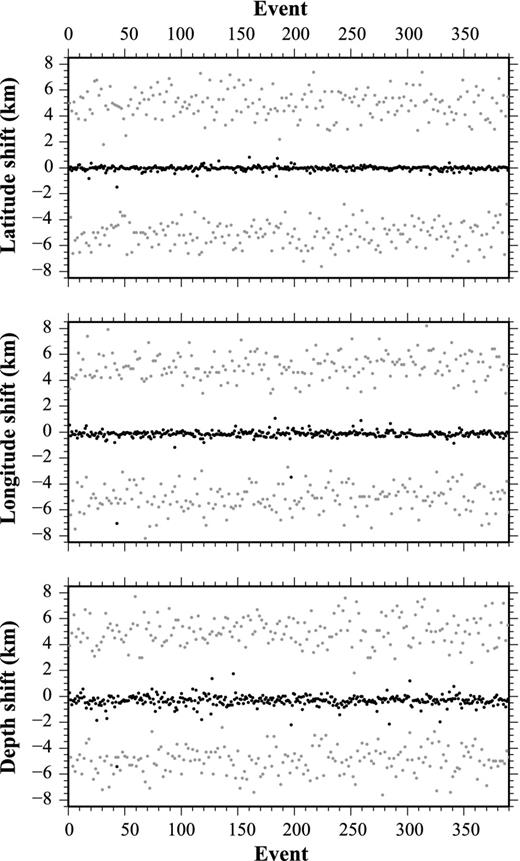
Test of VELEST location stability. Initial hypocentre locations, used as reference, are randomly perturbed with a shift of ±5 km. Grey dots represent the amount of shift (along latitude, longitude and depth) with respect to the reference locations. The inversion is then repeated, and the retrieved locations shifts are shown as black dots.
The retrieved ‘minimum 1-D velocity model’ presents a P-wave velocity, shallow layer (down to 2 km depth) of 3.2 km s−1 (Fig. 4b black line). This is consistent with the average P-wave velocity value due to different lithologies present in this depth range, varying from Carbonate Platform rocks (P-wave velocity of 5.3–6.0 km s−1) to thrust sheet-top clastic sequence (P-wave velocity of 2.0–2.4 km s−1; Improta et al.2003). The second 4-km-thick layer (from 2 to 6 km in depth) is characterized by a velocity of 4.7 km s−1 compatible with the seismic velocity of the Lagonegro Basin units (Improta et al.2003). The transition to the domains of Apulian Platform occurs gradually, passing through a 2-km-thick layer with a velocity of 5.5 km s−1. The retrieved velocity value of 6.2 km s−1 at 8 km and 6.5 km s−1 at 12 km of depth are compatible with previous studies (Improta et al.2003; Boncio et al.2007). Then the velocity smoothly increases with depth, up to a value of about 7 km s−1 at 14 km of depth. The lack of events for depth larger than 15 km (Fig. 4c) indicates that the velocity model is not resolved for depths below this value.
To account for local deviations from the 1-D velocity model, station corrections are computed during the inversion procedure. Positive and negative values of station correction—with respect to a reference station—correspond to local low- and high-velocity anomalies, respectively, in the vicinity of the recording station. VELEST allows for the use of station elevations during inversion, and rays are traced to the true station position. This is an important constraint since in the study area, the elevation of the recording sites ranges from 0.450 to 1.350 km a.s.l.
Station corrections are computed with respect to a reference station, CSG3, whose delay is close to zero (Fig. 6a). We chose this station because it lies towards the middle of the network, has a large number of readings with a small error on the observation and is located in an area where the surface geology is known. The spatial distribution of station corrections shows a significant lateral variation in the direction orthogonal to the Apenninic chain (Fig. 6a): stations located in the southwestern part of the region show early P-wave arrivals (negative station delays), while stations located in the northeastern part of the area show delayed P arrivals (positive delays). This large-scale pattern suggests that station corrections may be related not just to the shallow structures beneath each station, but also to strong lateral velocity variations in the deeper part of the crust. This is consistent with the known transition between the carbonate platform outcrops at Southwest and the Miocene sedimentary basins at Northeast.
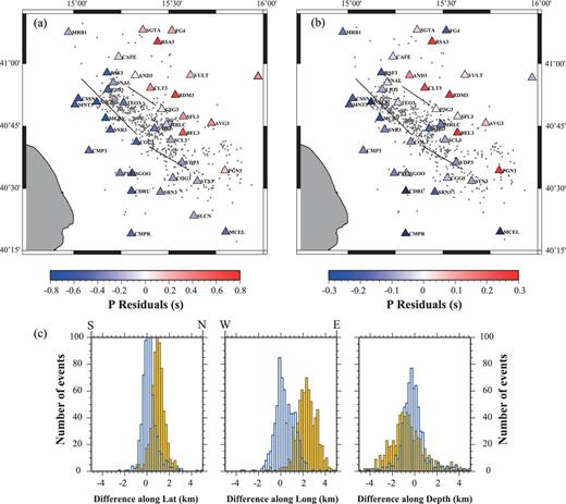
(a) Station corrections (colour-coded triangles) obtained from the VELEST inversion, along with the retrieved epicentral locations. (b) Improved station corrections, obtained by fixing the location of well-constrained reference hypocentres. Epicentral locations with this new set of station corrections are shifted back towards SE. (c) Histograms of the differences along latitude, longitude and depth between 1-D and 3-D hypocentral locations. 1-D locations are obtained either with station corrections shown in (a) yellow histogram, or with the improved station corrections shown in (b) blue histogram. 3-D locations are obtained in the model shown in Fig. 7.
This observation motivated us to use a preliminary 3-D P-wave tomographic velocity model—which is currently under validation—in order to: (1) clarify the relationship between station corrections and crustal velocity heterogeneities; (2) improve the quality of station corrections by using well-constrained reference events, relocated in the 3-D model. In the following section we will briefly discuss how the tomographic P-wave velocity model has been determined. More details (and further validation of the model) will be provided in an upcoming manuscript, which is currently in preparation.
5 3-D P-WAVE VELOCITY MODEL
A 3-D crustal velocity model is obtained from the tomographic inversion of the same data set of first P-wave arrival times. The inversion is performed using an improved method based on the accurate finite-difference traveltime computation and a simultaneous inversion of both velocity models and earthquake locations (Latorre et al.2004; Vanorio et al.2005; Battaglia et al.2008). We follow an iterative scheme by which a linearized delay-time inversion is performed. First arrival traveltimes of wave fronts are computed through a finite-difference solution of the eikonal equation (Podvin & Lecomte 1991) in a fine grid of 0.5 × 0.5 × 0.5 km3. The latter consists of constant slowness cells computed by tri-linear interpolation from the inversion grid. For each event–receiver pair, traveltimes are recalculated by numerical integration of the slowness on the inversion grid field along the rays traced in the finite-difference traveltime field (Latorre et al.2004). Simultaneously, for each node of the inversion grid, traveltime partial derivatives are computed for the P slowness field, hypocentre location and origin time. The parameters are inverted using the least squares root (LSQR) method of Paige & Sanders (1982); the number of inversion steps is set to a maximum of 20. Model roughness is controlled by the requirement that the Laplacian of the slowness field must vanish during the inversion procedure (Menke 1989; Benz et al.1996). The misfit function, defined as the sum of the squared time delay, is a posteriori analysed and the convergence is usually reached after 10 to 15 iterations.
The velocity model is parametrized by a nodal representation, described by a tridimensional grid. Different grid spacing has been tested, and in particular we performed several inversions progressively decreasing the distance of each node corresponding to increasing the number of parameters. We chose the optimal parametrization according to the minimum of the Akaike Information Criterion (Akaike 1974). The minimum is obtained for the model with 6 × 6 × 2 km3 grid spacing. Phase residuals reduction is about 68 per cent with a final rms value of 0.1 s.
The tomographic image clearly indicates the presence of a strong velocity variation in the upper 8–10 km depth of the crust, along the direction orthogonal to the Apenninic chain, so defining two domains characterized by relatively low (3.5–4.8 km s−1) and high (5.2–6.5 km s−1) P velocities, respectively (Fig. 7a).
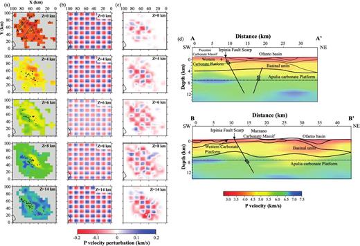
Preliminary 3-D tomographic model from the inversion of the data set analysed in this study. (a) Plan-view map at different depths of the velocity model, as absolute velocity values. The regions that are not covered by ray paths have been masked in grey. Triangles are station locations; black dots are hypocentral locations of the analysed events, AA′ and BB′ are the traces of the sections shown in (d). (b) Synthetic pattern for different depths added to the 3-D final tomographic model for the checkerboard test. (c) Map view at different depths for the checkerboard test results. (d) P-wave tomographic cross-sections with superimposed schematic geological section, proposed by Improta et al. (2003). See panel (a) for the trace of the sections. Black lines represent the fault segments of the 1980 Ms 6.9 Irpinia earthquake, as proposed by Pantosti & Valensise (1990). The colour-bar is referred to the panels (a) and (d).
To verify the spatial resolution of the inferred 3-D final velocity model, standard checkerboard tests were performed. The checkerboard model consists of an alternating pattern of positive and negative anomalies superimposed to the final model, in order to keep the same ray coverage (Fig. 7b). The anomalies are well resolved down to about 15 km of depth, and especially in the central part of the investigated area (Fig. 7c). However, lateral smearing is observed where ray distribution is not dense enough to reconstruct small features.
In Fig. 7(d), two vertical cross-sections of the P-wave velocity model are superimposed to a schematic geological section proposed by Improta et al. (2003). The picture shows that the inferred velocity model well reproduces the main geological features. Specifically, the top of the ACP between 6 and 7 km of depth is well identified by the high-velocity anomaly, whose values range from 6.0 to 6.8 km s−1. The sedimentary basinal units to the NE are well correlated with the shallow low-velocity anomaly (3.5–4.5 km s−1). The retrieved values are in agreement with those obtained by Improta et al. (2003).
6 STATION CORRECTIONS AND EARTHQUAKE RELOCATION
A qualitative comparison between the retrieved 3-D Vp anomalies (Fig. 7) and the spatial distribution of station corrections obtained so far (Fig. 6a ) confirms that the latter reflect large-scale geological changes. In fact, the spatial pattern of station corrections is coherent with the strong lateral P-wave velocity variation, in the direction orthogonal to the Apenninic chain, between 2 and 4 km (transition between the WCP and the Basinal Units) and between 4 and 8 km (topography of the Apulia Carbonate Platform).
To check the quality of station corrections, we compare the location of 670 earthquakes (with at least five P-wave and two S-wave arrival readings, and gap <200º) obtained in the 1-D model, using station corrections, with that obtained in the 3-D model. For both models, earthquake location is performed using a probabilistic, non-linear, global-search earthquake location method (NonLinLoc—Lomax et al.2009). This code follows the probabilistic formulation of the inverse problem of Tarantola & Valette (1982) and Tarantola (1987). The location code allows for the use of 3-D velocity models and produces accurate uncertainty and resolution estimates. The spatial probability density function obtained by the grid search algorithm represents the complete probabilistic solution of the earthquake location problem, including the information on uncertainty and resolution. Traveltimes between each station and the nodes of a 0.5 × 0.5 × 0.5 km3 grid are computed using a 3-D version of the eikonal finite differences scheme of Podvin & Lecomte (1991).
In order to use S-wave arrivals for location, a Vp/Vs ratio of 1.85 has been chosen as the value that minimizes the location rms. This value is in agreement with those obtained by other studies in the same region (Vp/Vs = 1.83 ± 0.40 in Maggi et al.2009; Vp/Vs = 1.8 ± 0.1 in Bernard & Zollo 1989; Amato & Selvaggi 1993; Bisio et al.2004; De Matteis et al.2010), and it is not far from the value obtained by our preliminary ‘modified Wadati diagram’ analysis (1.885).
Looking at the difference between observed and computed traveltimes as a function of the epicentral distance (Figs 8c and d), one can see that earthquake locations in the 3-D model better explain the observed P and S arrival times, over the whole range of distances. Following Shearer (1997) we compute, for the two location results, the parameters Wp and Ws, defined as the difference between the 75th and 25th percentiles in the histogram of P and S residuals, respectively. The largest value of Wp and Ws are found for the 1-D velocity model (Wp = 0.19 s, Ws = 0.42 s) corresponding to the greatest scatter in the residuals. This scatter is reduced in the 3-D model (Wp = 0.17 s, Ws = 0.40 s). We take, therefore, the 3-D hypocentral locations (shown in Figs 8a and b) as reference, and, based on those, we assess the quality of 1-D locations and station corrections. The yellow histograms in Fig. 6(c) show the differences (in latitude, longitude and depth) between 1-D and 3-D locations. One can see that 1-D epicentral locations are systematically shifted towards NE, with respect to 3-D locations, and therefore closer on average to the NE stations. This has the effect of reducing the theoretical traveltime to those stations and increasing the value of station correction (which is tobs − ttheo). Similarly, the SW stations are farther, on average, from the epicentres, which increases the theoretical traveltime and further reduces the station correction value for these stations. It seems, therefore, that a trade-off exists between a systematic epicentral shift towards NE and the relatively high values of station corrections (between −0.7 and 0.7 s) that we retrieve.
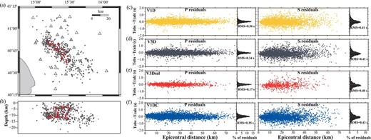
(a) Epicentral map of the selected earthquakes located in the 3-D tomographic model. (b) E–W vertical section of the 3-D–located hypocentres. Red dots in (a) and (b) are a subset of well-constrained hypocentres, used as reference events for improved station corrections computation. (c) Traveltime location residuals (difference between observed and computed traveltimes) for different velocity models, represented as a function of the hypocentral distance and as histogram, for P-wave (left-hand side) and for S-wave (right-hand side) arrivals. (c) V1D: location residuals for the retrieved 1-D model with the original station corrections. (d) V3D: location residuals for the 3-D tomographic model. (e) V3Dsel: location residuals for the selected earthquakes (in red in panel a and b) in the 3-D model. (f) V1DC: location residuals for the retrieved 1-D model with improved station corrections.
To check this hypothesis, we recomputed station corrections by fixing the position of well-constrained hypocentres, obtained from the 3-D location. We chose, as reference, 84 events (Figs 8a and b in red) having gap smaller than 70°, location error smaller than 5 km and at least eight P-wave and five S-wave readings. These events are clearly characterized by smaller residual dispersion (Fig. 8e) with respect to the whole data set (Fig. 8d).
Station corrections are recomputed using VELEST and fixing the velocity model and the hypocentral locations. New station corrections, and corresponding epicentral locations, are shown in Fig. 6(b). The difference between the new 1-D locations and the 3-D locations is shown by the blue histograms in Fig. 6(c). The new 1-D locations do not show systematic shifts anymore and, as consequence, station corrections are lower in amplitude, while retaining the same large-scale pattern. The distribution of traveltime residuals as a function of the epicentral distance for the 1-D location with improved station corrections is shown in Fig. 8(f).
In Fig. 9(a) we compare the spatial distribution of station corrections with the geological features of the area: negative values of station corrections are observed in correspondence of the carbonate platform outcrops at Southwest, while positive values correspond to the sedimentary basins at Northeast. Fig. 9(b) shows that station corrections are also correlated with the topography of the top of the ACP [determined by Improta et al. (2003) through a joint interpretation of gravity data, seismic reflection lines and deep wells information]. The doming of this tectono-stratigrafic unit in the Frigento area (NW of the studied region), with a minimum depth of 1 km, is associated to the large negative station correction at RSF3. The deepening of the ACP in the Ofanto Synform area, where thrust sheet-top syntectonic clastic sequences prevail at the surface, is compatible with the presence of positive values of station corrections at CLT3, RDM3 and BEL3. The largest positive value of station corrections in this area is reached in correspondence to the maximum depth of the ACP top (around 6 km).
7 DISCUSSION AND CONCLUSIONS
Earthquakes often occur in regions of complex geology, making it difficult to determine their locations due to uncertainty in path effects. Usually a 3-D velocity model can account for most of the traveltime anomalies that are not included in a 1-D model. However, 1-D models are sometimes a necessary—if not preferred—choice, for routine earthquake location, double-difference relocation, source parameter computation, Green's function calculation and as a starting point for 3-D tomographic analyses.
In this work we retrieved a robust and reliable 1-D reference P-wave velocity model—together with well-defined traveltime station corrections—for a structurally complex area (Campania–Lucania region), from the analysis of background regional seismicity (M < 3.5). The procedure consisted in: (1) determining a P-wave ‘Minimum 1-D velocity model’ with station corrections, using VELEST (Kissling et al.1995); (2) retrieving a preliminary 3-D crustal velocity model, using an iterative linearized scheme (Latorre et al.2004; Vanorio et al.2005); (3) using improved 3-D earthquake locations to redefine 1-D station corrections, thus resolving the trade-off between earthquake locations and station corrections introduced in step (1).
The final 1-D model, with station corrections is presented in Tables 1 and 2. The model is characterized by a Vp = 3.2 km s−1 shallow layer (down to 2 km of depth), whose velocity is consistent with the average P-wave velocity value related to the different surface lithologies in the area, which vary from Carbonate Platform domain at SW to thrust sheet-top clastic sequence at NE. The second layer, 4 km thick, with Vp = 4.7 km s−1, is compatible with the depth range and the seismic velocity of the Lagonegro Basin units. A transition to the domains of ACP that occurs gradually passing across a layer of 2 km (Vp = 5.5 km s−1), is observed. The retrieved velocity value of 6.2 km s−1 at 8 km and 6.5 km s−1 at 12 km of depth are compatible with previous studies (Improta et al.2003; Boncio et al.2007). Then the velocity smoothly increases with depth, up to a value of about 7 km s−1 at 14 km of depth.
‘Minimum’ 1-D velocity model. In the first column are indicated the depth of the top (km) for each layer. In the second column the P-wave velocity value (km s−1).
| Top of layer (km) | Vp (km s−1) |
|---|---|
| −1.5 | 3.25 |
| 2.0 | 4.72 |
| 6.0 | 5.51 |
| 8.0 | 6.20 |
| 12.0 | 6.55 |
| 14.0 | 6.70 |
| 22.0 | 6.80 |
| 30.0 | 6.85 |
| 35.0 | 7.03 |
| Top of layer (km) | Vp (km s−1) |
|---|---|
| −1.5 | 3.25 |
| 2.0 | 4.72 |
| 6.0 | 5.51 |
| 8.0 | 6.20 |
| 12.0 | 6.55 |
| 14.0 | 6.70 |
| 22.0 | 6.80 |
| 30.0 | 6.85 |
| 35.0 | 7.03 |
Station corrections. In the first and third columns are indicated the name of stations. In the second and fourth columns are indicated the P-residual values (s).
| Stations | P-residuals (s) | Stations | P-residuals (s) |
|---|---|---|---|
| AND3 | 0.1243 | TEO3 | −0.0401 |
| AVG3 | 0.0751 | VDP3 | −0.1103 |
| BEL3 | 0.5081 | VDS3 | −0.1866 |
| CGG3 | −0.0657 | CAFE | −0.0371 |
| CLT3 | 0.2397 | CDRU | −0.3986 |
| CMP3 | −0.1282 | CMPR | −0.4505 |
| COL3 | −0.1086 | CSSN | −0.1878 |
| CSG3 | 0.0000 | FG4 | −0.2091 |
| LIO3 | −0.0832 | MCEL | −0.3845 |
| MNT3 | −0.2156 | MCRV | −0.2601 |
| NSC3 | −0.4334 | MRB1 | −0.1544 |
| PGN3 | 0.3707 | MRLC | −0.1467 |
| PST3 | −0.1374 | PALZ | −0.0754 |
| RDM3 | 0.4992 | PTRP | 0.2407 |
| RSA3 | 0.2781 | SGO | −0.0682 |
| RSF3 | −0.2223 | SGTA | 0.0585 |
| SCL3 | −0.0932 | SNAL | 0.0028 |
| SFL3 | −0.0294 | VULT | 0.0346 |
| SNR3 | −0.1334 | MRN3 | −0.3454 |
| SRN3 | −0.2098 | SALI | −0.0529 |
| STN3 | −0.1018 |
Station corrections (Table 2) are integral part of our 1-D velocity model. Their large-scale spatial pattern shows strong lateral variation in the direction orthogonal to the Apenninic chain, which is consistent with the transition between the carbonate platform outcrops at Southwest and the Miocene sedimentary basins at Northeast. Moreover, a comparison of station corrections values with the top of the ACP shows a correspondence between the highest and lower values and the regions where the top of the platform is deepened and rises, respectively. These observations are strengthened by a 3-D tomographic image that further confirms the presence of a strong velocity variation along the direction orthogonal to theApenninic chain. It should be emphasized that the deep NE, rather deep, sedimentary basins are clearly visible in the tomographic image.
From the relocation of the events in the new model, we were able to retrieve an optimal Vp/Vs ratio, as the value that minimizes the location rms. We interpret the high Vp/Vs value of 1.85 as due to the presence of a fractured rock volume, partially water-saturated.
As a final step, to better interpret the distribution of seismicity in the area, we further relocated our data set using the double-difference technique (HypoDD—Waldhauser & Ellsworth 2000; Waldhauser 2001). Relative locations from double-difference further minimize errors related to un-modelled velocity structures, under the assumption that ray paths from the events to a common station are similar. This assumption is verified, in our case, since hypocentral separation is small compared to the event–station distance and to the length scale of the velocity heterogeneities.
911 earthquakes (from the initial data set consisting of 1312 events) could be successfully relocated. The epicentral distribution of the relocated seismicity is shown in Fig. 10(a). The present low-magnitude seismicity along the Apennine chain is not associated to single structures but rather to a volume comprised between the main faults activated during the 1980 M 6.9 earthquake (Fig. 10b). The principal stress direction, computed from focal mechanisms (De Matteis et al.2012), is nonetheless compatible with anti-Apenninic extensional regional stress field. This cloudy distribution of background seismicity is likely related to stress perturbation and volumetric damaging associated to the reloading process of main faults. Occasional repeated earthquakes and swarm-like microearthquake sequences have been observed within the region (Stabile et al.2012), pointing at specific zones of high stress concentration that correspond to mechanical asperities and/or to faster loading/unloading processes. The background seismicity in the Potenza area delineates an E–W-striking dextral strike-slip structure that cuts off the NW–SE–striking normal faults along the Apennine chain. This evidence is consistent with results obtained by Ekstrom (1994) and Di Luccio et al. (2005), who previously analysed the 1990 and 1991 earthquake sequences. The bimodal trend of depth distribution of seismicity (Fig. 10c) has been explained by Boncio et al. (2007) in terms of crustal rheology, which consists of a strong brittle layer at mid-crustal depths, sandwiched between two plastic horizons.
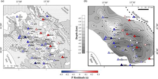
Comparison of improved station corrections with (a) a schematic geological map of Campania–Lucania region, and (b) the topography of the top of the Apulian Carbonate Platform (from Improta et al.2003).
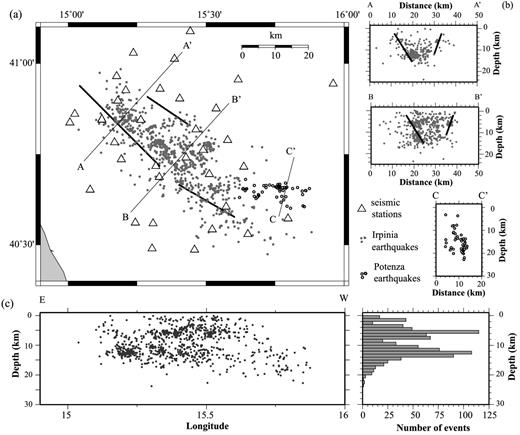
(a) Map view of the seismicity from 2005 August to 2011 April relocated through double-difference method, using the 1-D velocity model obtained in this study. Events along the Apenninic chain are represented with light grey circles, while the events in the Potenza region are represented with open circles. Black lines are the surface projection of the three fault segments that ruptured during the 1980 Irpinia earthquake (Pantosti & Valensise 1990). (b) Cross-sections of the seismicity along the profiles reported in the map. Black lines represent the projection of the fault segments of the Irpinia earthquake. (c) E–W vertical section of the seismicity and histogram of the events as function of depth.
To conclude, a reference 1-D velocity model for the Campania–Lucania region was a necessary requirement for current routine operations at the ISNet network and for future refined seismological studies. We introduced a robust and reliable model obtained by careful selection and repicking of 1312 small-magnitude earthquakes. The a posteriori validation, through the comparison with a preliminary 3-D tomographic model, shows that significant bias can exist between earthquake locations and station corrections, leading to systematic shifts in hypocentral positions. An independent strategy to check location quality seems therefore to be a required step when deriving ‘minimum 1-D models’.
8 DATA AND RESOURCES
Data can be obtained from the ISNet Bulletin at http://seismnet.na.infn.it (Elia et al.2009; last accessed November 2011) and from the INGV data management centre http://iside.rm.ingv.it/iside/standard/index.jsp (last accessed December 2011).
Most of the figures were made using Generic Mapping Tools software (Wessel & Smith 1998; http://gmt.soest.hawaii.edu/ last accessed March 2013).
The research has been partially funded by REAKT [European Community's Seventh Framework Programme (FP7-ENV-2011) under grant agreement n. 282862] and GEISER [European Community's Seventh Framework Programme (FP7-ENERGY-2009-1) under grant agreement n. 241321] projects.
We thank the editor, Prof. Xiaofei Chen, and two anonymous reviewers for their constructive considerations. Moreover, we acknowledge Dr. Mauro Caccavale (KNMI), Dr. Tony Alfredo Stabile (IMAA-CNR) and all the members of the seismological laboratory of the Department of Physics (University of Naples Federico II) for useful discussions and comments.
Now at: Laboratoire de Géologie, École Normale Supérieure, CNRS, Paris, France.
Now at: Istituto Nazionale di Geofisica e Vulcanologia, Osservatorio Vesuviano, Napoli, Italy.
