


Abstract
How do body-wave traveltimes constrain the Earth's radial (1-D) seismic structure? Existing 1-D seismological models underpin 3-D seismic tomography and earthquake location algorithms. It is therefore crucial to assess the quality of such 1-D models, yet quantifying uncertainties in seismological models is challenging and thus often ignored. Ideally, quality assessment should be an integral part of the inverse method. Our aim in this study is twofold: (i) we show how to solve a general Bayesian non-linear inverse problem and quantify model uncertainties, and (ii) we investigate the constraint on spherically symmetric P-wave velocity (VP) structure provided by body-wave traveltimes from the EHB bulletin (phases Pn, P, PP and PKP). Our approach is based on artificial neural networks, which are very common in pattern recognition problems and can be used to approximate an arbitrary function. We use a Mixture Density Network to obtain 1-D marginal posterior probability density functions (pdfs), which provide a quantitative description of our knowledge on the individual Earth parameters. No linearization or model damping is required, which allows us to infer a model which is constrained purely by the data.
We present 1-D marginal posterior pdfs for the 22 VP parameters and seven discontinuity depths in our model. P-wave velocities in the inner core, outer core and lower mantle are resolved well, with standard deviations of ∼0.2 to 1 per cent with respect to the mean of the posterior pdfs. The maximum likelihoods of VP are in general similar to the corresponding ak135 values, which lie within one or two standard deviations from the posterior means, thus providing an independent validation of ak135 in this part of the radial model. Conversely, the data contain little or no information on P-wave velocity in the D′′ layer, the upper mantle and the homogeneous crustal layers. Further, the data do not constrain the depth of the discontinuities in our model. Using additional phases available in the ISC bulletin, such as PcP, PKKP and the converted phases SP and ScP, may enhance the resolvability of these parameters. Finally, we show how the method can be extended to obtain a posterior pdf for a multidimensional model space. This enables us to investigate correlations between model parameters.
1 INTRODUCTION
Since the start of the 20th century, the illumination of the Earth's interior by seismic waves has enabled seismologists to infer its seismic velocity and density structure. Current 3-D tomographic models show structural variations in great detail (see e.g. Nolet 2008; Rawlinson et al.2010, for an overview). Such tomographic inversions are often built upon radial (1-D) earth models. The quality of a 3-D tomographic model is thus intrinsically linked to the robustness of a 1-D model; therefore, it is crucial to assess the quality of the latter. Further, seismological models are frequently used to determine earthquake locations. The spherically symmetric ak135 model (Kennett et al.1995), for instance, is used in the location algorithm of the International Seismological Centre (ISC). However, any imperfections in the earth model will map into the source location estimate (e.g. Valentine & Trampert 2012b). Clearly, an accurate estimation of seismic source parameters requires a precise knowledge of the underlying earth model and its uncertainties. However, determining the quality of earth models is non-trivial.
In many geophysical inverse problems, a single ‘optimal’ solution is obtained via a linearized approach (e.g. Parker 1994; Tarantola 2005). In reality, the dependence of the data on the model often is non-linear. Further, not all model parameters are equally resolved by the data, and seismological inversions usually suffer from a strong model non-uniqueness (e.g. de Wit et al.2012). Therefore, it is important to understand the uncertainties and resolution associated with the one ‘optimal’ model. Neglecting these is likely to lead to flaws in any interpretation of the final model. Various approaches are available to assess model quality. For instance, Kennett et al. (1995) used a non-linear search procedure to assess the robustness of the spherically symmetric ak135 model in the lower mantle and core, but the velocity bounds for the search procedure itself were based on the final model and relatively narrow, that is, within 0.5 per cent from ak135. de Wit et al. (2012) showed how to explore the model null-space to investigate the non-uniqueness of a 3-D tomographic model. Alternatively, a resolution analysis is often employed to investigate the robustness of the inferred Earth structure, using for instance the linear framework provided by Backus & Gilbert (1968, 1970). For example, the resolution of 1-D density structure, as determined from normal mode data, was investigated using both linear (Masters & Gubbins 2003) and non-linear techniques (Kennett 1998). However, it would be better to take the non-linearity and model non-uniqueness into account in our inversion framework, rather than treating them ex post facto.
A more general approach, which allows us to solve a non-linear inverse problem and to quantify uncertainties, involves the description of our knowledge about earth parameters by probability distributions (e.g. Tarantola & Valette 1982; Tarantola 2005). Following Bayes’ theorem (Bayes 1763), our posterior knowledge of the model is our prior knowledge updated by the observed data, using a physical theory that relates the model to the data. The aim of Bayesian inference is to obtain the posterior probability distribution σ(m|d) of the model m, conditioned on the observed data d. A common approach is to directly sample the posterior model probability density using Monte Carlo techniques (e.g. Mosegaard & Tarantola 1995; Sambridge 1999a,b; Resovsky & Trampert 2003; Käufl et al.2013). Beghein et al. (2006) constructed probability density functions (pdfs) to assess whether radial anisotropy in existing 1-D mantle models is robust. While such sampling methods are powerful for solving non-linear inverse problems, they quickly deteriorate as the dimension of the model space increases, a phenomenon which Bellman (1961) termed the curse of dimensionality. In practice, this currently limits the use of sampling methods to inverse problems which involve at most a few tens of model parameters.
As an alternative to Monte Carlo techniques, we use artificial neural networks to solve the Bayesian inverse problem. Neural networks can be viewed as non-linear filters and are very common in pattern recognition problems. They can approximate an arbitrary non-linear relation between two parameter spaces, inferring the mapping from a set of training data. As such, neural networks can be very useful in situations where the forward relation is known, but the inverse mapping is unknown or difficult to establish by more conventional analytical or numerical methods. This situation applies to many geophysical inverse problems. In addition, neural networks can interpolate between available model samples, as opposed to conventional Monte Carlo methods, which only sample the model space discretely. This helps to address the dimensionality issue mentioned above. Common references on artificial neural networks include Bishop (1995) and MacKay (2003).
Neural networks are widely applied in many different research areas, such as finance, medicine and engineering. Applications include bankruptcy risk predictions (e.g. Odom & Sharda 2002), breast cancer detection (e.g. Baker et al.1995), face recognition (e.g. Rowley 1998), landslide susceptibility estimation (e.g. Lee et al.1998) and traffic flow forecasting (e.g. Jiang & Adeli 2005). Extensive reviews of geophysical applications of neural networks are given by van der Baan & Jutten (2000) and Poulton (2002). Recent examples include Devilee et al. (1999) and Meier et al. (2007a, 2009), who invert surface wave phase velocities for (local) Earth structure, and Shahraeeni & Curtis (2011) and Shahraeeni et al. (2012), who infer petrophysical parameters from seismic velocity data on the reservoir scale. Valentine & Woodhouse (2010) use neural networks for the quality assessment of seismic waveforms, while Valentine & Trampert (2012a) investigate neural network-based dimensionality reduction of seismograms and its potential applications.
Here we perform a Bayesian inversion of P-wave traveltime curves for the Earth's spherically symmetric P-wave velocity (VP) structure. We use traveltimes from the EHB bulletin (Engdahl et al.1998) for the Pn, P, PP and PKP phases. The inverse problem is non-linear, as the ray paths of the seismic phases depend on the underlying velocity structure of the Earth. Our focus is twofold. First, we demonstrate how to solve a Bayesian non-linear inverse problem and assess model uncertainties using neural networks. Second, we quantify the constraint on radial VP structure which is provided by the traveltime data for these major seismic phases. To solve our non-linear inverse problem, we use a particular class of neural networks, known as a Mixture Density Network (MDN, Bishop 1995). An MDN outputs a parametric distribution, which approximates the continuous posterior model probability density. This distribution reflects our updated state of knowledge on the earth model parameters.
First, we briefly outline the Bayesian inversion framework, followed by an introduction to artificial neural networks. Second, we describe the model parametrization and the traveltime data used for this study. Last, we invert the traveltime data using neural networks and show the 1-D marginal pdfs for P-wave velocity parameters and discontinuity depths. We emphasize that our focus lies on the constraints on individual model parameters; we do not present a new 1-D earth model.
2 METHODOLOGY
2.1 The inverse problem
2.2 Neural networks
An artificial neural network is essentially a mathematical model of an arbitrary mapping between two parameter spaces. By changing the free parameters of the mathematical model, during a so-called training process, the mapping can be modified to represent the desired relation. Network training is driven by presenting the network with examples of corresponding input–output pairs. The fundamental idea is to represent the potentially complicated mapping as a combination of many simpler univariate activation functions. Common choices for the activation functions are the logistic and hyperbolic tangent functions. We use the latter in this work, because symmetric sigmoids, such as the hyperbolic tangent, often display better convergence properties during network training (e.g. LeCun et al.1998). It is the non-linear nature of such functions that helps neural networks to approximate non-linear relations.
2.2.1 The Multilayer Perceptron (MLP)
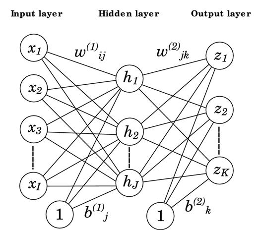
A two-layer feed-forward Multilayer Perceptron (MLP). The lines represent the two layers of free parameters in the network, represented by the weights |$w_{ij}^{(1)}$| and |$w_{jk}^{(2)}$| and biases |$b_{j}^{(1)}$| and |$b_{k}^{(2)}$|. The I input neurons xi feed into the J hidden neurons hj, which form the input to the K output units zk. An additional input of value 1 feeds into the hidden and output layer, which is associated with the biases. Information flows only from the input to the output neurons (feed-forward).
Learning corresponds to the minimization of a cost function with respect to the network weights. The cost function measures the difference between the network output and the desired output, the target vector. The necessary derivatives are given by the backpropagation algorithm, as introduced by Werbos (1974) and Rumelhart et al. (1986). The network is trained on a synthetic data set D = {xn, tn}, where n = 1, …, N labels the statistically independent patterns in the data set. Every pattern consists of a pair of input and target vectors x and t, respectively. Once successfully trained, the network can be applied to unseen input to produce an estimate of the unknown output.
2.2.2 The Mixture Density Network
Bishop (1995) shows that an MLP, as shown in Fig. 1, outputs the mean of the conditional probability distribution p(t|x) of the target t, conditioned on the input x. This will give meaningless results if the underlying function, which relates input and target, is multivalued; therefore, it is desirable to obtain the full conditional distribution of the target (e.g. Bishop 1995; Meier et al.2007a). We thus employ an MDN, which can model an arbitrary probability distribution, in the same fashion that an MLP can approximate an arbitrary function (McLachlan & Basford 1988).
Fig. 2 illustrates an MDN, as introduced by Bishop (1995). The parameters describing the mixture model form the output z(d; w) of a conventional MLP, as shown in Fig. 1. For M spherical Gaussian kernels, the MLP will have (c + 2) · M output parameters. Alternatively, more complex Gaussian kernels, such as Gaussians with full covariance matrices (Williams 1996), could be used. This is computationally more demanding, however, and we find that spherical kernels are flexible enough to model the probability densities of interest here. See Bishop (1995) for a detailed description of the MDN.
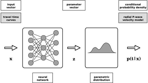
A Mixture Density Network (MDN), as introduced by Bishop (1995). The output of an MDN approximates a parametric distribution p(t|x) for the target t, conditioned on the input x. The parameters describing this distribution are given by the output z of a neural network, such as the MLP shown in Fig. 1. In this study, the input consists of traveltime data d, while the target represents the parameters of interest m′, which form a subspace of the l-dimensional radial P-wave velocity earth model m (eqs 1 and 2).
2.2.3 Network training
MDN training corresponds to the minimization of the cost function in (eq. 7). Commonly, gradient-based optimization algorithms are used for this task. We use the Scaled Conjugate Gradient (SCG) algorithm (Møller 1993), which avoids the expensive line-search procedure of the conjugate gradient algorithm. Conjugate gradient methods acquire second order information about the error surface and are therefore more efficient than simpler gradient descent methods.
Gradient-based optimization methods typically operate iteratively and thus require a user-defined starting point for the network weights. The starting point is crucial to ensure that the network training converges to an appropriate solution. For the hyperbolic tangent function, the summed input should be of order unity. If not, the activation functions become saturated, that is, their first derivative tends to zero. Consequently, the error surface will become almost flat, so that training ceases to be useful. To aid the initialization of the training process, it is common practice to pre-process the input and target vectors (Appendix A).
The initial network weights are drawn from a Gaussian distribution of zero mean. The variance of this distribution is inversely proportional to the number of input units I for the first layer weights |$w_{ij}^{(1)}$| and the number of hidden units J for the second layer weights |$w_{jk}^{(2)}$| (Bishop 1995). Further, the network parameters are initialized such that σ(m′|d, w) ≈ ρ(m′), that is, the initial posterior pdf resembles the prior pdf. This requires setting some initial values for the biases of the output layer in the MLP (|$b_{k}^{(2)}$| in Fig. 1). Following (Bishop 1995; Nabney 2002), such an initialization leads to faster convergence and reduces the risk of the optimization method getting stuck in a poor local minimum.
Regardless of the initialization, every network run will be sensitive to the specific initial network parameters. It is therefore common practice to train multiple networks with different random weight initializations, all other settings being equal. The optimal weight vector w*, which minimizes the cost function (eq. 7), is used to estimate the marginal posterior pdf σ(m′|d, w*) through eq. (5).
2.2.4 Generalization and regularization
The goal of network training is to approximate the relationship between two parameter spaces. Such a mapping is in general believed to be found when the optimal network produces accurate results for previously unseen data, that is, data that was not used for network training. In that case, the network is said to display a good generalization behaviour. This can be verified by using a data set that is independent of the training data.
To simulate the presence of measurement uncertainties in the real data, noise is added to the synthetic data. This discourages the network from fitting the details of the training data set, referred to as overfitting. Instead, it enhances the generalization behaviour by encouraging the network to map the underlying relation between input and output. Bishop (1995) shows that such noise addition is similar to using a regularization constraint (such as simple weight decay), thereby forcing the network to find a smooth mapping, that is, a mapping that is insensitive to variations in the data on the order of the noise level. Meier et al. (2007a) demonstrate this concept in the context of a Bayesian inversion of surface wave data.
In addition, we employ early stopping, which is a common procedure to improve generalization. The network is trained using the conventional training set, but training is halted when the error (eq. 7) for an independent validation set starts to increase. Since the validation set is used to determine the optimal set of network weights, a third (test) set is used to verify the accuracy of the network on unseen data.
3 MODEL PARAMETRIZATION
We adopt a piecewise continuous representation for the P-wave velocity model, as was used for the prem (Dziewonski & Anderson 1981) and iasp91 (Kennett & Engdahl 1991) models. The piecewise continuous functions can be used to evaluate the model at any depth exactly. We parametrize the depths of seven discontinuities in the VP profile: the inner core boundary (ICB) and core–mantle boundary (CMB), the top of the D′′ layer, the discontinuities around 660, 410 and 210 km depth and the Moho. We define the lower mantle (LM) as the region between the top of the D′′ layer and the 660 km discontinuity, while the transition zone (TZ) spans the region between the 660 and 410 km discontinuities.
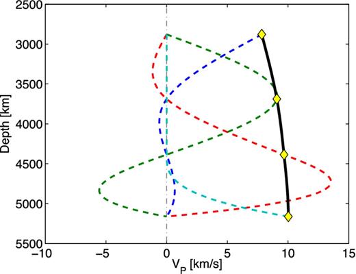
An example of the natural cubic splines used to construct the 1-D earth models, following eq. (8). The coefficients ai represent VP values in the outer core (yellow diamonds), drawn from the prior model distribution ρ(m). The black line shows the resulting VP profile f (z) in the outer core, which is constructed by summing the products aiψi(z) for the four splines (dashed).
The transition zone and the region between the 410 and 210 km discontinuities are parametrized using eq. (8) with L = 2. This results in linear velocity gradients with depth in these layers. We separate the region between the Moho and 210 km discontinuity in two linear (L = 2) segments, that is, 210–120 km and 120–Moho km, as the linear velocity gradient in these two segments differs significantly in existing 1-D models such as ak135. Thus, the velocity profile is continuous at 120 km depth, but its first derivative is not. The depth of the transition at 120 km is not varied. The lower mantle and outer core are parametrized by 4 knots, and the inner core by 3, which results in non-linear gradients with depth (Fig. 3). The crust is parametrized by two homogeneous layers. No sediment or water layers are present. We thus have 29 parameters in our model m: 22 VP parameters (the coefficients ai in eq. 8) and 7 discontinuity depths.
Tables 1 and 2 define the prior model distribution ρ(m) (eq. 1). Discontinuity depths are independently drawn from uniform priors, as are the VP values directly below the discontinuities (Table 1). The prior distributions are centred on the corresponding values of the ak135 model. We choose conservative priors by allowing for a large variation in the independent model parameters, that is, ±3 per cent with respect to ak135 for VP in the core and lower mantle and ±5 per cent in the upper mantle. We emphasize that by choosing such broad prior distributions, we ensure that the results of our probabilistic inversion are not driven by the actual values in the ak135 model.
Prior information on independent model parameters. Prior distributions are uniform over the specified ranges. The ranges for the P-wave velocity parameters are given as percentile perturbations from ak135 (Kennett et al.1995), except for VP in the two crustal layers. VP parameters are indicated by |$m^{1}_{d}$| and represent the knots located directly below a discontinuity d. Note that the tops of the transition zone (TZ) and the lower mantle (LM) are formed by the 410 and 660 km discontinuities, d410 and d660, respectively. The interpolation style for the VP profile in every region, following eq. (8), is given in the last column.
| Discontinuity | Parameter | Range (km) | |
|---|---|---|---|
| Inner–outer core (ICB) | dICB | 5133.5–5173.5 | |
| Core–mantle (CMB) | dCMB | 2871.5–2911.5 | |
| D′′ layer (top) | |$d_{D^{\prime \prime }}$| | 2720–2760 | |
| 660 discontinuity | d660 | 630–690 | |
| 410 discontinuity | d410 | 380–440 | |
| 210 discontinuity | d210 | 190–230 | |
| Moho | dMoho | 25–75 | |
| Region | Parameter | Range (± per cent) | Interpolation style |
| Inner core (IC) | |$m^{1}_{{\rm IC}}$| | 3 | 3 cubic splines |
| Outer core (OC) | |$m^{1}_{{\rm OC}}$| | 3 | 4 cubic splines |
| D′′ layer | |$m^{1}_{D^{\prime \prime }}$| | 3 | Linear |
| Lower mantle (LM) | |$m^{1}_{{\rm LM}}$| | 3 | 4 cubic splines |
| Transition zone (TZ) | |$m^{1}_{{\rm TZ}}$| | 5 | Linear |
| 410–210 | |$m^{1}_{210}$| | 5 | Linear |
| 210–Moho | |$m^{1}_{{\rm Moho}}$| | 5 | |
| 210–120 | Linear | ||
| 120–Moho | Linear | ||
| Region | Parameter | Range (km s−1) | |
| Lower crust (LC) | mLC | 6.4–7.4 | |
| Upper crust (UC) | mUC | 5.6–6.3 |
Prior information on dependent model parameters. Prior distributions are uniform over the specified ranges, which are given as percentile perturbations from the updated model value (see text). The indices |$m^{i}_{d}$| represent the correlated model parameters in every region d, with higher indices i corresponding to deeper VP knots in the parametrization. The corresponding independent parameters |$m^{1}_{d}$| are listed in Table 1.
| Region | Parameter | Range (± per cent) |
|---|---|---|
| Inner core (IC) | |$m^{2,3}_{{\rm IC}}$| | 1 |
| Outer core (OC) | |$m^{2,3,4}_{{\rm OC}}$| | 1 |
| D′′ | |$m^{2}_{D^{\prime \prime }}$| | 1 |
| Lower mantle (LM) | |$m^{2,3,4}_{{\rm LM}}$| | 1 |
| Transition zone (TZ) | |$m^{2}_{{\rm TZ}}$| | 2 |
| 410–210 | |$m^{2}_{210}$| | 2 |
| 210–Moho | |$m^{2,3}_{{\rm Moho}}$| | 2 |
The VP values at the other L − 1 knots in each region are calculated using the new value at the first knot (|$m_{d}^{1}$| in Table 1) and the gradient of the ak135 model. Subsequently, these values are perturbed, with the amount of perturbation drawn from a uniform prior (Table 2). This introduces a correlation between the VP parameters in each region. In general, radial P-wave velocity increases with depth, that is, the velocity gradient is mostly positive. By using the gradient in ak135, we aim to exclude physically implausible models and restrict the size of our model space.
We generate 99 862 synthetic models, which are drawn from the prior model distribution ρ(m). Ten synthetic models in the training set are shown in Fig. 4, along with the ak135 model. Note that locally negative velocity gradients can still exist in the models.
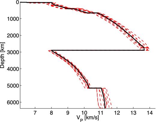
Ten model realizations (red), drawn from the prior distribution ρ(m) and ak135 (black) for VP.
4 TRAVELTIME DATA
4.1 EHB data
The EHB bulletin (Engdahl et al.1998) contains millions of routinely determined traveltime measurements, which have been corrected for source mislocation. We select traveltime data for the Pn, P, PP, PKPab, PKPbc and PKPdf phases for the years 2001–2008 (Fig. 5). For simplicity, we exclude PnPn, the upgoing phases pP, pwP and sP and the crustal phases Pb and Pg.
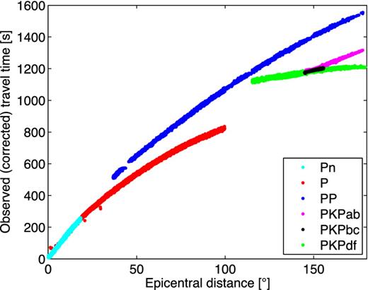
Travel time measurements in the EHB bulletin for 2001–2008. Event depths are restricted to lie between 14 and 16 km.
Several corrections are provided with the EHB bulletin. We correct the raw EHB data for the Earth's ellipticity and station elevation. We do not apply the regionally smoothed station corrections, which perform regional averaging (5 × 5° patches) to smooth out effects of lateral heterogeneities in the upper mantle. In our setup, the imprint of 3-D structure on the traveltime measurements is treated as noise; therefore, such a correction is unnecessary here.
We select the traveltimes for which the EHB estimated source depth lies between 14 and 16 km. Note that this range of depths is chosen to approximate a fixed source around 15 km depth and not to represent the uncertainty in EHB source depth estimates; we will discuss our data noise model below in Section 4.3. Each event in the EHB bulletin is given a three-letter label that characterizes the quality of hypocentral determination. We exclude the EHB measurements for which the source depth is fixed to a standard depth by Engdahl, denoted by FEQ in the EHB data, and solutions for which the uncertainty in source depth is expected to be >15 km (LEQ, XEQ). The remaining data correspond to 1100 events that were registered at 5268 different stations (Fig. 6). Both sources and receivers are globally distributed, that is, within the typical limitations of seismological data coverage.

Locations of 1100 sources (red asterisks) and 5268 stations (green dots) in the EHB data for 2001–2008. Event depths are restricted to lie between 14 and 16 km.
4.2 Synthetic data
Neural network training and validation requires a data set containing many examples of input–output pairs. For this purpose, we calculate synthetic first-arrival traveltime curves for 99 862 synthetic models using the TauP package (Crotwell et al.1999). The synthetic models are parametrized as described in the previous section. All 29 model parameters are allowed to vary in each model realization. The source depth is fixed to 15 km for all synthetic data. Thus, source depth is a fixed parameter in our setup and any uncertainties in EHB depth estimates are regarded as a source of data noise, as will be discussed below in Section 4.3. The three PKP branches are calculated separately. Travel times are computed for a phase-specific range of epicentral distances at one degree intervals (Table 3). For these phases, the distance ranges are comparable to those used by Kennett et al. (1995), who used traveltime data collected by the ISC. We include Pn, which refracts along the Moho, to provide a better constraint on the structure of the uppermost mantle.
Epicentral distance range for the seismic phases. The ranges used by Kennett et al. (1995) are added as a reference.
| Distance range (°) | Pn | P | PP | PKPab | PKPbc | PKPdf |
| This study | 3:18 | 25:88 | 50:173 | 145:174 | 145:155 | 122:179 |
| Kennett et al. (1995) | – | 25:99 | 53:180 | 156:178 | 151:153 | 118:180 |
| Distance range (°) | Pn | P | PP | PKPab | PKPbc | PKPdf |
| This study | 3:18 | 25:88 | 50:173 | 145:174 | 145:155 | 122:179 |
| Kennett et al. (1995) | – | 25:99 | 53:180 | 156:178 | 151:153 | 118:180 |
If for a given distance no arrival is computed by TauP, the traveltime is set to zero. By doing so, the number of elements in every traveltime branch is constant. This is a requirement of the network architecture, which only permits input vectors of constant dimension. The zeros represent gaps in the traveltime curves, which commonly result from low-velocity zones, and associated negative gradients, in the earth model. This information is therefore available to the neural network. Note that for the epicentral distance ranges used (Table 3), no gaps occur in the globally distributed EHB data (Fig. 5). This could indicate that there are no global low-velocity zones in the parts of the Earth sampled by the data, or that some of the EHB traveltimes do not represent a direct geometric arrival (or a combination of both).
4.3 Data uncertainties
Uncertainties exist in both the epicentral distance, through the source location estimate, and the traveltime measurements. We add noise to the synthetic data to simulate these two types of uncertainty.
For every synthetic traveltime measurement, we draw a perturbation to the epicentral distance from a uniform distribution |$\mathcal {U}(-\epsilon _{{\rm dist}},+\epsilon _{{\rm dist}})$| with ϵdist = 0.1°( ∼ 10 km). The value of ϵdist is similar to the average test-event mislocation reported by Engdahl et al. (1998). The corresponding traveltime is updated by applying the local gradient in the traveltime curve to this perturbation.
Second, the synthetic data have to be corrupted to reflect noise in the traveltime data. The scatter in the observed traveltime data (Fig. 5) originates from lateral heterogeneities in the Earth, measurement errors, phase misidentifications and uncertainties in the estimated source depth. For a given phase p and epicentral distance i, we estimate the noise as the spread in the EHB traveltimes. The half-width of this spread ϵip (Fig. 7) is used to define a Gaussian noise distribution |$\mathcal {N}(0,\epsilon _{ip}^{2})$|, that is, with zero mean and standard deviation ϵip. A random sample from this noise distribution is added to every synthetic datum. The scatter in the data may be small if few data are available, which would result in an unrealistically low noise estimate. Therefore, we impose a minimum phase-specific noise level (Table 4), which is based on measurement error estimates documented in a recent ISC report (ISC 2008).
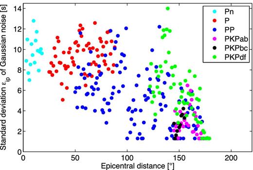
The half-width of the spread in the observed traveltimes ϵip is used as the standard deviation of the Gaussian noise model, which differs for every phase p and epicentral distance i. Different colours denote different phases.
4.4 Data processing
The input d to the neural network is a concatenation of the traveltime curves for the different phases. Since the curves are rather smooth, a large (linear) correlation exists between the traveltime at different epicentral distances. Therefore, we sample the traveltime curves at intervals of 2°. This reduces the size of the input vector and thus the number of network parameters, thereby making network training faster. In light of the strong correlations, we assume that this downsampling does not result in a significant loss of information on our earth model. The resulting input vector consists of 152 traveltimes, which is a concatenation of the data for the Pn (8 traveltime measurements), P (32), PP (62), PKPab (15), PKPbc (6) and PKPdf (29) phases.
For every synthetic model, the input pattern is constructed by sampling the synthetic data at 2° intervals and subsequently adding a random noise sample (Fig. 8). The input vectors for the observed data are constructed in a slightly different fashion. For each distance sample dip, with phase p and epicentral distance i, we extract all observations from the EHB data for which the epicentral distance lies within the range dip ± ϵdist, where ϵdist = 0.1° as before. Consequently, multiple EHB observations are available at each distance point. We draw one random sample from these multiple possibilities. This yields the EHB traveltime curves that serve as input to the trained networks (Fig. 9). The differences between these curves are regarded as noise (see Section 4.3). The variations in the real data vectors are significantly smaller than the variations in synthetic training patterns (cf. Fig. 8). Both observed and synthetic data contain noise, but the variations in the synthetic data are larger due to the differences in the underlying synthetic earth models.
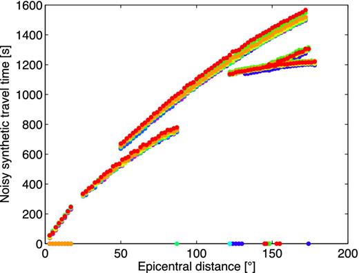
Examples of noisy synthetic traveltime data that form the input to the network. The synthetic data are sampled at distance intervals of 2° for the epicentral distance ranges specified in Table 3. Note the zeros in the traveltime curves, which indicate that TauP did not compute an arrival at the corresponding distance.

Note that upon applying a trained network to one input pattern for the EHB data, only 152 measurements are ‘inverted’. For a given distance and phase, however, all available observations should contain the same information on the radial earth model, given the measurement noise defined above. When repeated with a different EHB input pattern, constructed as described here, the inversion should yield similar results.
5 RESULTS
We present inversion results for all 22 P-wave velocity and seven discontinuity depth parameters. For each model parameter mi, we investigate the constraint that is provided by the traveltime data and quantify the associated uncertainty. We therefore train MDNs on 1-D target vectors m′ = mi (eq. 2). Since all model parameters are allowed to vary in the synthetic models, the output of each MDN forms a 1-D marginal posterior pdf σ(mi|d). This is equivalent to marginalizing the full joint posterior pdf σ(m|d) over all model parameters other than mi via the integration in eq. (2). σ(mi|d) reflects our knowledge of mi given the variations in the other 28 model parameters.
5.1 Network configuration
For all results presented in this study, we train MDNs with 40 hidden units and a Gaussian mixture consisting of 15 Gaussian kernels (M = 15). We verified that the precise number of hidden units is not of paramount importance to final network performance. The same applies to the number of Gaussian kernels. During training, the mixing coefficient αj can be set close to zero for redundant kernels, or kernels can be combined by having a similar mean and variance (Bishop 1995).
For a 1-D target (c = 1), the MDN has (c + 2) · M = 45 output parameters: the means μj, the variances |$\sigma _{j}^{2}$| and the mixing coefficients αj (eqs 5 and 6). In combination with the 152-D input pattern (Figs 8 and 9), the corresponding MLP has 7725 free parameters (the weights |$w_{ij}^{(1)}$| and |$w_{jk}^{(2)}$| and biases |$b_{j}^{(1)}$| and |$b_{k}^{(2)}$| in Fig. 1). We use 80 per cent of the 99 862 patterns in the synthetic data set for training, 15 per cent for the validation set, which is used to evaluate the early stopping criterion, and the remaining 5 per cent for the test set.
Theoretically, there is no limit to the size of a neural network. However, a larger network consists of more free parameters and thus takes longer to train. More importantly, more network parameters require a larger training set to succesfully train the network. Therefore, computational facilities restrict the network size. In general, the number of free parameters should not exceed the number of training patterns (e.g. Bishop 1995; Duda et al.2001). In this study, we ensure that the training set is approximately a factor of 10 larger than the number of network parameters. The main computational requirement thus lies in the generation of synthetic training patterns, that is, repetitively solving the forward problem. For the ∼100 000 patterns, this took ∼100 hr on a standard desktop computer. Once the training set is available, network training is relatively fast: the training time for a single network is on the order of tens of minutes in this study.
Due to the random initialization of the network weights, the optimization algorithm can become stuck in local minima of the error surface. To verify that network training converges properly, we train 30 independent networks. For each of these networks, training commences at a different point in weight space due to the random initialization. To reduce the chance of overfitting, all synthetic patterns are divided randomly over the training, validation and test sets before the training of each independent network commences. We find that results for the 30 independent networks are similar and choose the network that produces the lowest pattern-averaged error for the test set.
5.2 Network evaluation
For each VP parameter, we apply the optimal MDN to the ∼5000 patterns in the synthetic test set, which are not used for network training. Network performance can be evaluated by comparing the resulting ∼5000 1-D marginal pdfs with the true synthetic model value. As an example, we show 1-D marginal posterior pdfs for one test pattern for three model parameters: VP directly above the ICB, directly above the 210 km discontinuity and in the lower crust (Fig. 10). For the P-wave velocity near the ICB (left-hand frame) and 210 km discontinuity (middle frame), most probability mass in the posterior distribution lies close to the target value (black line). We conclude that network performance is accurate for this particular input pattern. It is clear from the marginal pdf of VP in the lower crust (right-hand frame) that the traveltime data do not constrain this part of the model. Consequently, the MDN output represents the uniform prior distribution for this parameter. The difference between the MDN output and the true uniform prior pdf is due to the fixed shape of the finite number of Gaussian kernels.
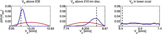
1-D marginal posterior pdf (blue line), prior pdf (red) and true model value (black, dashed) for one pattern in the test data set for VP (left-hand frame) directly above the ICB, (middle frame) directly above the 210 km discontinuity and (right-hand frame) in the lower crust.
It is difficult to quantitatively evaluate network performance from such marginal distributions, however. A more pragmatic validation method is to analyse the correlation between the target value and the mean of the dominant Gaussian kernel in the MDN output (Bishop 1995). We take the kernel associated with the largest mixing coefficient αj (eq. 5) to be dominant. Although this simple measure ignores the information provided in the full posterior pdf, such an analysis provides a practical way of evaluating the trained networks.
For all 22 VP parameters, Fig. 11 shows the mean μj of the dominant Gaussian kernel versus the true target value for all patterns in the test data set. Every row in the figure represents a region between two discontinuities, with the depth of the VP parameter (knot) decreasing from left to right. The corresponding correlation coefficient R is given above every frame (R = 0 indicates no correlation, whereas R = 1 represents a perfect correlation). Network performance on these unseen input patterns is good (R ≥ 0.87) for the P-wave velocity in the inner and outer core and lower mantle (first, second and fourth row, respectively). For VP in the D′′ layer (third row), the upper mantle (fifth and sixth row) and crust (bottom row), correlations are in general low or absent (R ≈ 0).
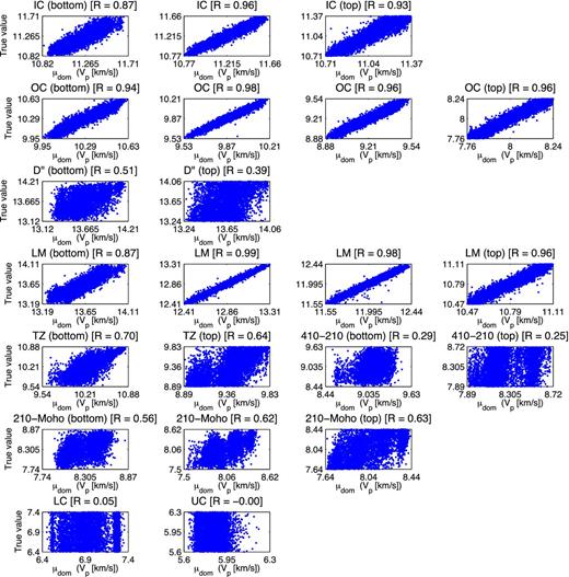
Mean μj (eq. 6) of the dominant Gaussian kernel (maximum αj in eq. 5), labelled μdom in the figure, versus the true synthetic value for all patterns in the test data set for the 22 VP parameters (Tables 1 and 2). The regions between discontinuities are displayed on different rows. For every region, depth decreases from left to right in the figure. The corresponding correlation coefficient R is given above each frame.
Besides network evaluation, the performance on synthetic input is a good indicator of the constraint that the data provide on the model. For the P-wave velocity directly above the ICB, for instance, the 1-D marginal posterior pdf is unimodal and narrow relative to the width of the prior pdf (left-hand frame, Fig. 10). This parameter is constrained well by the data, as indicated by R = 0.94 in Fig. 11 (second row, first column). Conversely, for VP in the lower crust the mean of the ‘dominant’ kernel does not relate to the true value (R = 0.05, Fig. 11, seventh row, first column). The traveltime data do not constrain this part of the model, as is apparent from the corresponding marginal pdf in Fig. 10 (right).
One can expect similar results, for both resolved and unresolved model parameters, when applying the trained networks to the observed traveltime data. As the data provide very little or no constraint on the seven discontinuity depth parameters, we do not show the corresponding performance on the test set here and restrict ourselves to the application to the EHB data for these parameters.
5.3 Application to EHB data
Fig. 12 shows 1-D marginal pdfs for P-wave velocities for the ten EHB input patterns in Fig. 9. Recall that these ten input patterns are random realizations from the available EHB data set, as described in Section 4.4. The differences between these input patterns are regarded as noise. The network should be insensitive to such variations, since we have used a similar noise level during network training. Consequently, network output should be approximately the same for these different input vectors.
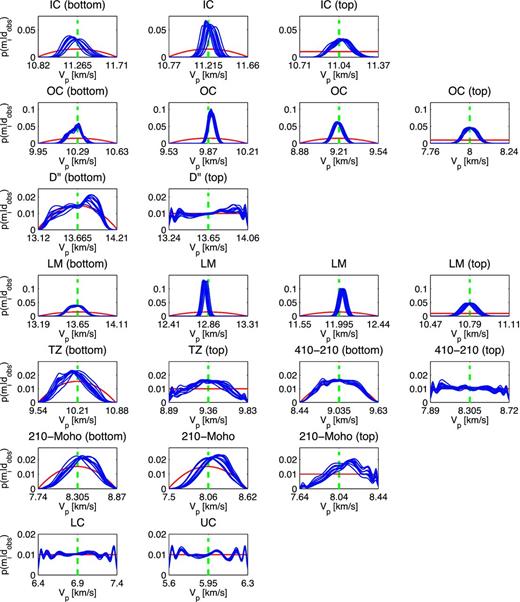
1-D marginal posterior pdf (blue line), prior pdf (red) for the 22 VP parameters (Tables 1 and 2). The same trained networks as used for Fig. 10 are applied to ten different EHB input patterns (Fig. 9). The regions between discontinuities are displayed on different rows. For every region, depth decreases from left to right in the figure. Note that the range of the vertical axis, that is, normalized probability, differs between rows.
The data constrain VP in the outer core (OC) and lower mantle (LM) best (second and fourth row, respectively). PKPdf, the only seismic phase in our data set that is sensitive to the inner core (IC), constrains VP in this region (first row). The most notable feature is the proximity of the posterior maxima to the ak135 values, which are indicated by the green dashed lines. However, in addition to a most likely model value, we obtain uncertainties in the P-wave velocity estimate. Recall that our posterior pdfs are based on our conservative prior pdfs and are therefore taken to be independent of the actual values in the ak135 model.
For each VP parameter in the inner core, outer core and lower mantle, we extract statistics from the ten posterior distributions in Fig. 12. Since the ten distributions are similar for these parameters, we calculate the mathematical expectation 〈VP〉 and standard deviation |$\sigma _{V_{P}}$| of the 10 pdfs combined (Table 5). When expressed as a percentage of the mean 〈VP〉, the standard deviation of the posterior pdfs |$\sigma _{V_{P}}$| is smaller than 1 per cent for every model parameter. The corresponding ak135 values are given as a reference and lie within one standard deviation from 〈VP〉 for the parameters in Table 5, except for |$m_{{\rm LM}}^{2,3}$| in the lower mantle, for which ak135 lies within two standard deviations. It is difficult to compare the uncertainties found here, represented by the standard deviations |$\sigma _{V_{P}}$|, as uncertainty estimates are scarce in the literature. Kennett et al. (1995) used a non-linear search procedure to evaluate a range of models around ak135 for various data misfit measures. They used velocity bounds of ±0.02 km s−1 for the lower mantle and ±0.04 km s−1 for the lowermost mantle and core. The |$\sigma _{V_{P}}$| values we find here are on the order of these velocity bounds or a factor of 2–3 larger (Table 5). We emphasize that our uncertainty estimates are not representative of the uncertainties in ak135, given the differences in the data selection and the model parametrization. However, the constraint on individual model parameters, as investigated here, may be indicative of the uncertainties in ak135 and similar models.
Mean 〈VP〉 and standard deviation |$\sigma _{V_{P}}$| of the ten 1-D marginal posterior pdfs for the P-wave velocity parameters (Fig. 12) in the inner core (IC), outer core (OC) and lower mantle (LM). All values are in (km s−1), except for the fourth column, which shows the standard deviation |$\sigma _{V_{P}}$| as a percentage of the mean 〈VP〉. The corresponding value in ak135 is given for comparison (|$V_{P}^{ak135}$|). Recall that the depth of the knots mi decreases with decreasing index number i (see Tables 1 and 2).
| Parameter | 〈VP〉 | |$\sigma _{V_{P}}$| | |$\sigma _{V_{P}}$| (per cent) | |$V_{P}^{ak135}$| |
|---|---|---|---|---|
| |$m^{3}_{{\rm IC}}$| | 11.248 | 0.107 | 0.952 | 11.265 |
| |$m^{2}_{{\rm IC}}$| | 11.229 | 0.066 | 0.589 | 11.215 |
| |$m^{1}_{{\rm IC}}$| | 11.063 | 0.081 | 0.736 | 11.040 |
| |$m^{4}_{{\rm OC}}$| | 10.266 | 0.056 | 0.545 | 10.290 |
| |$m^{3}_{{\rm OC}}$| | 9.899 | 0.030 | 0.304 | 9.870 |
| |$m^{2}_{{\rm OC}}$| | 9.201 | 0.043 | 0.466 | 9.210 |
| |$m^{1}_{{\rm OC}}$| | 8.004 | 0.041 | 0.506 | 8.000 |
| |$m^{4}_{{\rm LM}}$| | 13.638 | 0.086 | 0.629 | 13.650 |
| |$m^{3}_{{\rm LM}}$| | 12.819 | 0.031 | 0.239 | 12.860 |
| |$m^{2}_{{\rm LM}}$| | 12.034 | 0.039 | 0.320 | 11.995 |
| |$m^{1}_{{\rm LM}}$| | 10.793 | 0.057 | 0.528 | 10.790 |
The 1-D marginals for VP between the Moho and the 210 km discontinuity (Fig. 12, sixth row) indicate that the traveltime data contain some information on this region. We find that this is mainly due to the addition of the Pn phase, which refracts along the Moho. The data indicate a (very) weak preference for velocities slightly higher than in ak135. We should point out, however, that the posterior distributions include all but the very low P-wave velocities. Thus, for these model parameters the data cannot falsify any of the assumptions on VP contained in our model prior.
The data contain no or at most a very limited signal on the parameters of the D′′ layer (third row, Fig. 12), the transition zone (TZ, fifth row), the region between the 410 and 210 km discontinuities (410–210, fifth row) and the two homogeneous crustal layers (seventh row). The poor constraint on upper mantle structure is not surprising, given the teleseismic epicentral distances for which P (above 25°) and PP (above 50°) traveltimes are used (Table 3).
The traveltime data we invert here contain practically no information on the depth of the discontinuities (Fig. 13). For the upper mantle, this may be explained by the near-vertical incidence under which the teleseismic rays travel through the discontinuities in this region. The inclusion of phases that reflect of discontinuities, for example, PcP, which reflects of the CMB, could improve the constraint on discontinuity depths.

6 DISCUSSION
We trained neural networks to invert P-wave traveltime data for the radial P-wave velocity structure of the Earth. We obtained a continuous probabilistic description of the individual model parameters from the conjunction of our prior knowledge with the information contained in the data. The 1-D marginal posterior pdfs enable us to assess the uncertainty in the model parameters, which reflects the non-uniqueness of the non-linear inverse problem.
A visual comparison of the prior and posterior pdfs enables us to assess how well a model parameter is resolved by the data. Alternatively, one can quantify the constraint on a model parameter by comparing the information content of the prior and posterior pdfs (Tarantola & Valette 1982), as was done by for instance Meier et al. (2007b). Quantifying the information content, or gain, is useful when quantitatively comparing the resolving power of various data types or when it is not possible to show the posterior pdfs for all model parameters. We do not include such a measure in this study, as we explicitly show the prior and posterior distributions for all 29 model parameters (Figs 12 and 13).
We use neural networks as an alternative to Monte Carlo methods. A succesful comparison of the two types of technique was presented by for instance Meier et al. (2007a); Shahraeeni & Curtis (2011). The ∼100 000 samples in our data set can be used to sample the posterior pdf with the straightforward Independent Metropolis–Hastings algorithm. However, we find that the data set is insufficient to produce robust results. To obtain the posterior pdf, we would need many more samples or a more sophisticated approach, such as the Neighbourhood Algorithm (Sambridge 1999a). This illustrates the efficiency of the neural network to interpolate between the limited number of available samples
In general, the deeper parts of the model (inner and outer core, lower mantle) are constrained well by the data and the corresponding posterior pdfs contain VP values similar to those in ak135 (Kennett et al.1995). By contrast, the same data provide little information on the upper mantle VP structure and the depth of discontinuities in the radial VP profile. Kennett et al. (1995) derived the ak135 model from the traveltime data provided by the ISC. They used the same phases as we use here, except for Pn, and in addition used PcP, PKKP, P′P′ (PKPPKP) and the converted phases ScP and SP. The inclusion of such complimentary phases could have enhanced our knowledge on parts of the VP model. These phases, however, are not included in the EHB bulletin for 2001–2008 and we decided to restrict our inversion to the phases listed in Table 3.
Ideally, the output for all ten input patterns in Figs 12 and 13 is similar (see Section 4.4). This is the case for the well-resolved parameters in the outer core and lower mantle. Differences between the posterior pdfs are larger for the inner core parameters, as they are for the P-wave velocity in the uppermost mantle (210–Moho). The trained networks are thus not completely insensitive to random variations in the input on the order of the noise level. In our view, however, these differences are minor and we argue that similar inferences would be drawn from the ten 1-D marginal posterior pdfs for these parameters.
For all parameters, the networks have been trained on the same type of traveltime data as input. Obviously, any information redundancy between the individual units in the input pattern is inefficient from the perspective of network training. This is the case for the inner core parameters, for which we know only PKPdf carries information. It would thus be most efficient if the networks trained for the inner core parameters would only take PKPdf as input. We verified that prediction accuracy is similar, regardless of whether the networks are trained on the full input pattern or only on PKPdf traveltimes. Thus, network training is able to focus on the systematic relation between the PKPdf data and the inner core P-wave velocities.
Our final results comprise the 1-D marginal posterior pdfs σ(mi|d) of the model parameters mi. These represent all available knowledge on the individual model parameters, given the traveltime data, associated measurement errors, our choices regarding the model parametrization and the variations in the other model parameters. Such 1-D distributions do not contain information on any correlations between model parameters. Further, we emphasize that the maximum likelihood values of the individual model parameters, when taken together, do not necessarily represent the maximum likelihood model. Therefore, it is often desirable to analyse the joint posterior pdf, that is, the posterior probability distribution of the full model σ(m|d) (eq. 1). This distribution could be obtained by training a network on the complete 29-D model m. Such a network, however, would contain a lot of free parameters and thus require a large training set. Further, network training may converge slowly or not at all for such a high-dimensional target space.
As a simple example, we construct 2-D marginal posterior pdfs using eq. (9), that is, for a 2-D m′ (eq. 2), for one of the patterns in the test set. Fig. 14 shows the three distributions in eq. (9) for two different combinations of parameters: VP at the top of the inner core (|$m_{{\rm IC}}^{1}$|) and the ICB depth dICB (first row) and VP in the lower mantle (|$m_{{\rm LM}}^{1}$| and |$m_{{\rm LM}}^{2}$|, second row). The inner core VP is resolved well, whereas the ICB depth is unresolved, as was apparent from the 1-D marginals in Figs 12 and 13. No correlation between these parameters is observed in the 2-D marginal pdf (Fig. 14). The two shallowest VP parameters in the lower mantle are resolved well (cf. Fig. 12, fourth row). Despite the good constraint provided by the data, a (weak) positive correlation between the two parameters is visible in the corresponding 2-D marginal posterior pdf (Fig. 14).
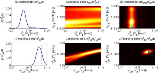
Construction of 2-D marginal posterior pdfs via eq. (9) for (first row) VP at the top of the inner core (|$m_{{\rm IC}}^{1}$|) and the ICB depth (dICB) and (second row) VP in the lower mantle (|$m_{{\rm LM}}^{1}$| and |$m_{{\rm LM}}^{2}$|). See Tables 1 and 2 for the model parametrization. The three panels in each row show (left-hand panel) the 1-D marginal pdf, (middle panel) the conditional pdf and (right-hand panel) the 2-D marginal pdf for one of the patterns in the test set. Lighter colours denote higher probabilities. The corresponding target values are denoted by the black line (left-hand panel) and the cyan star (right-hand panel).
7 CONCLUDING REMARKS
We used artifical neural networks to solve a non-linear Bayesian inverse problem. Neural networks are flexible and can be used to approximate an arbitrary function. No linearization or model damping is required, which allows for an optimal use of the information on the model that is contained in the data. We used an MDN to acquire a continuous probabilistic description of each model parameter. Each 1-D marginal posterior pdf represents our knowledge of the parameter and provides the necessary quantification of uncertainties, which plays a crucial role in any interpretation of seismological models.
We investigated the information on the Earth's radial P-wave velocity structure that is available in the EHB traveltime data for the Pn, P, PP, PKPab, PKPbc and PKPdf phases. Our results comprise 1-D marginal posterior probabiliy distributions for the 22 VP parameters and seven discontinuity depths in our model. These 1-D marginal pdfs enable us to assess the uncertainty in the individual model parameters. We have shown how the method can be extended to obtain a posterior pdf for a multidimensional model space. This enables us to investigate potential correlations between model parameters.
The P-wave velocities in the inner core, outer core and lower mantle are resolved well, that is, standard deviations of ∼0.2 to 1 per cent with respect to the means of the 1-D marginal posterior pdfs. The maximum likelihoods of VP are in general similar to the corresponding ak135 values, which lie within one or two standard deviations from the means of the posterior pdfs (Table 5). This provides an independent validation of this part of the ak135 model, which is often used in 3-D seismic tomography and earthquake location algorithms. Conversely, the data contain little or no information on P-wave velocity in the D′′ layer, the upper mantle and the homogeneous crustal layers. For the upper mantle, this is not surprising, given that the traveltime data used here are of a teleseismic nature, that is, >25° epicentral distance. Using additional phases available in the ISC bulletin, such as PcP, PKKP and the converted phases SP and ScP, may enhance the resolvability of our model parameters. However, the major phases we used here give a good indication of how much information on the radial VP structure is contained in typical body-wave traveltime data. We included Pn, which led to a weak constraint on the VP structure in the uppermost mantle. The data do not constrain the depth of the discontinuities in our model. Again, this is common knowledge, as teleseismic rays tend to travel perpendicular to discontinuities and thus provide a poor sampling of these structures. Reflected phases, such as PcP, which reflects of the CMB, are known to contain much more information on discontinuities.
Seismograms contain more information on the seismic source and the Earth's structure. We aim to apply Mixture Density Networks to Bayesian seismic waveform inversion in the future. However, for such an application the dimensionality of the data is much larger than for the traveltime inversion performed in this study, which presents additional challenges that must be overcome.
We thank Malcolm Sambridge and an anonymous referee for constructive reviews. We appreciate helpful discussions with Paul Käufl and Hanneke Paulssen. Ralph de Wit and Andrew Valentine are funded by the Netherlands Organization for Scientific Research (NWO) under the grant ALW Top-subsidy 854.10.002. Computational resources for this work were provided by the Netherlands Research Center for Integrated Solid Earth Science (ISES 3.2.5 High End Scientific Computation Resources).
REFERENCES
APPENDIX A: DATA PRE-PROCESSING
In addition to pre-processing the input, we find that it is beneficial to pre-process the target data and thus perform a similar operation as in eq. (A3) to the target data. Obviously, this linear transformation turns the targets into dimensionless numbers. Therefore, once the network is trained we reverse the linear transformation in eq. (A3) and apply it to the Gaussian kernel means |$\boldsymbol{\mu }_{j}$| and standard deviations σj in the MDN output (eq. 6). By doing so, these parameters are given in the true physical dimensions of the earth model parameters. We do not correct the standard deviations σj for the translation in eq. (A3), however, as the variance of a probability distribution is invariant under translations. The mixing coefficients αj are not transformed, as they are dimensionless and sum to one due to the application of the softmax function (Bishop 1995).
Note that the validation and test sets are pre-processed following eq. (A3) by using the mean xi and the variance Var(xi) calculated for the training data set (eqs A1 and A2). Thus the same transformation is applied to the three different synthetic data sets. The same is true for the observed data.
