


Abstract
Observations of the Earth's nutations provide constraints on the mechanical coupling at the core–mantle and inner core boundaries. An important physical mechanism that could be responsible for the observed dissipation is the electromagnetic (EM) coupling, to which this paper is devoted. Previous studies assumed that the main feature of the magnetic field that affects the EM coupling is its overall strength, its morphology being considered unimportant. In particular, these studies rely on the hypothesis that the contribution to the torque from all the non-dipolar components of the field can be approximated by the contribution that a uniform radial field with the same strength would have. In this study, we compute the EM torque for more realistic configurations of the magnetic field at the core boundaries and thereby assess the role of its spatial distribution on the strength of the EM torque. For field strengths typical of the core–mantle boundary (CMB), we show that the spatial distribution affects weakly the strength of the torque, with the approximation by a uniform field leading to an overestimation of the torque magnitude by ∼15–20 per cent. However, for field strengths typical of the inner core boundary (ICB), the morphology of the field has a more significant influence on the EM torque and the approximation by a uniform field overestimates the torque by ∼30–40 per cent. Assuming that EM coupling is responsible for the observed dissipation, we infer constraints on the strength of the radial magnetic field at both the CMB and ICB. We show how the unknown morphology of the magnetic field induces uncertainties on the estimated field strength at the ICB, which can take values anywhere in the range of ∼9–16 mT. These very large values suggest that EM coupling at the ICB cannot be the only mechanism responsible for the observed dissipation.
1 INTRODUCTION
Nutations are periodic variations in the orientation of the Earth's rotation axis in space. This motion is generated by the gravitational torque applied on the Earth's equatorial bulge by the Moon, the Sun and the other planets. Because the mantle, the fluid outer core and the solid inner core react differently to the applied torque, the nutation motion is characterized by differential rotations between these three regions. Since the boundaries of the fluid outer core are permeated by a background magnetic field (the geodynamo field), the differential rotation at the fluid core boundaries induces a secondary magnetic field by shear and advection of the background field. The associated electric currents produce Lorentz forces on both sides of the boundaries. These electromagnetic (EM) forces give rise to a net torque which tends to oppose the differential rotation and couples the rotation motion of the different regions.
If the background magnetic field at the boundary is weak, the secondary magnetic field induced by the differential rotation is also weak and the associated Lorentz force does not affect significantly the flow in the liquid outer core. The total motion of the fluid core can then be well described by a rigid-body rotation. In this case, Buffett (1992) showed that the magnitude of the EM torque is mainly determined by the electrical conductivity on both sides of the boundary and by the rms strength of the radial magnetic field at this boundary, whereas the morphology of the field has only a very small influence. In addition, in this ‘weak-field regime’, the contribution to the EM torque coming from the non-dipolar components of the field can be approximated, with an excellent precision, by the contribution that a hypothetical uniform radial field with the same rms strength would have.
However, for magnetic field strengths typical of the Earth's core, the induced field should be sufficiently large that the Lorentz force is expected to perturb the flow in the outer core from its rigid-body rotation. Therefore, this back reaction has to be taken into account when computing the EM torque at the core boundaries. The computation of the EM torque in this more general ‘strong-field regime’ was addressed by Buffett et al. (2002). Relying on results obtained in the weak-field regime, their model considered only two configurations of the radial magnetic field: a dipole field and a uniform field. The uniform field was assumed to represent the average contribution of the non-dipolar, short-wavelength, components of the field. However, the validity of this approximation has not been justified in the strong-field regime. It is not clear that a uniform radial field can capture equivalently the contribution of all the non-dipolar components to the EM torque when the back reaction of the Lorentz force plays an important role in the coupling dynamics.
Indeed, in a previous paper (Dumberry & Koot 2012), we have shown, for a particular example of a more complicated field configuration at the inner core boundary (ICB), that the torque can depart significantly from the one obtained from a uniform radial field. The first purpose of this paper is to compute the EM torque in the strong-field regime for several realistic configurations of the radial magnetic field, both at the core–mantle boundary (CMB) and at the ICB, and to assess the validity of the equivalent uniform radial field approximation.
Computations of the EM torque for realistic field configurations have been performed by Deleplace & Cardin (2006) when studying the coupling at the CMB. They concluded that the effect of the unknown small scales were rather small (lower than 10 per cent). However, their study only considered field strengths up to ∼0.4 mT, which is too small to explain the observed dissipation at the CMB by EM coupling alone. As we show in this paper, the effects of the field morphology on the EM torque become more important as the overall strength of the field gets larger. Therefore, the effect of field distribution could be larger than suggested by Deleplace & Cardin (2006) at the CMB. Moreover, at the ICB, where the field is expected to be much stronger than at the CMB, we expect these effects to become much more important.
A second objective of our paper is to infer constraints on physical properties of the Earth's core from nutation observations. In contrast to previous studies (e.g. Buffett et al.2002; Mathews et al.2002; Koot et al.2010), our model of EM coupling at the core boundaries takes into account realistic spatial configurations of the magnetic field, rather than an approximation of the field by the sum of a dipolar and uniform components. In particular, we compute uncertainties on the estimated physical parameters that are due to the unknown morphology of the magnetic field.
2 GENERAL BACKGROUND
2.1 Geomagnetic field
2.2 Nutation motion
2.3 EM coupling model
2.3.1 General formulation
Eqs (9)–(12) are equivalent to the equations derived by Buffett et al. (2002), although written in a form that relates explicitly the coupling constants to the physical parameters of the problem. This helps to get further insights into the problem. In particular, these equations show that the dependence of the torque on Br is complex as, in addition to the factor |$B_r^2$| in the integrals, Br also appears in the Elssasser number x±. Moreover, the dependence on Br is also coupled to the dependence on the electrical conductivities, as can be seen in eq. (12).
All the computations presented in this paper are performed using the model of Buffett et al. (2002), namely eqs (9)–(12). However, in order to get some intuition on how the magnetic field and the electrical conductivities affect the torque, it is interesting to compute, from eqs (9)–(12), approximate expressions that are valid in two limit cases. The first one corresponds to x± → 0 and the second one to x± ≫ 1. These limit cases are presented in the following sections.
2.3.2 Weak-field limit
Two important points can be made from eqs (15). First, the dependence of the coupling on the magnetic field goes simply as |$B_r^2$|. This means that the strength of the coupling is directly proportional to the mean-squared value of the radial field over the boundary: |$K_b \propto \bar{B}_r^2$|. Secondly, the dependence of the torque on the electrical conductivities on both sides of the boundary is entirely decoupled from the dependence on the magnetic field. The torque is simply inversely proportional to the sum of the of the square roots of the magnetic diffusivities.
2.3.3 Very strong-field limit
Eq. (17) shows that the dependence of the torque on the physical parameters is very different in this field strength regime than in the weak-field case. First, the dependence on the field strength is now linear: |$K_b \propto \bar{B}_r$| and, secondly, the EM torque is now independent of the electrical conductivities.
2.4 Physical properties of the core boundaries
Among the parameters that enter the EM torque in eqs (9)–(12), the least well known are the electrical conductivities on both sides of the boundaries and the radial magnetic field permeating them. Since it is our lack of knowledge on these parameters that inhibits a more precise determination of the torque, it is useful to summarize the information that we have on them from available observations and models.
2.4.1 Electrical conductivities
Estimates of the conductivity of the Earth's outer core can be obtained from laboratory experiments on liquid iron alloys at high pressure and temperature. However, these experiments cannot be carried out at the actual pressure and temperature of the Earth's core so that the results have to be extrapolated to core conditions. Using this technique, the outer core electrical conductivity has been estimated to be typically of the order of σf = 5 × 10⁵ S m−1 (Stacey & Anderson 2001). Recently, using theoretical computations based on density functional theory (ab initio computations), Pozzo et al. (2012, 2013) estimated that liquid iron alloys typical of outer core composition have a conductivity of σf = 1.1 × 10⁶ S m−1 at CMB conditions and σf = 1.3 × 10⁶ S m−1 at ICB conditions. Similar results have been obtained by de Koker et al. (2012). For the inner core, we make the assumption that its electrical conductivity σs is equal to that of the outer core at the ICB.
The electrical conductivity of the lowermost mantle σm also affects directly the EM coupling at the CMB. Typical silicates at the conditions of the lower mantle have been estimated from laboratory experiments to have a conductivity of the order of 10 S m−1 (e.g. Shankland et al.1993). However, there are several reasons for which a much larger conductivity on the mantle side of the CMB would be possible. First, it has been shown recently that FeO, which should be an important constituent of the lower mantle and which is an insulator at Earth's surface conditions, becomes metallic at the conditions of the lower mantle, with an electrical conductivity of 0.9 × 10⁵ S m−1 (Ohta et al.2012). Although this does not imply a continuous layer at the base of the mantle with such a large conductivity, the presence of metallic FeO certainly increases significantly the conductivity of the lowermost mantle. Another mechanism that could allow for a large electrical conductivity is the existence of chemical reactions between the silicate mantle and the liquid iron from the outer core. Laboratory experiments carried out at high pressure and temperature suggest that due to chemical interactions with the outer core, iron alloys could be present in the lower mantle (Knittle & Jeanloz 1989; Otsuka & Karato 2012). Therefore, depending on whether the lower mantle is mostly made of silicates or whether a significant amount of metallic elements are present, the electrical conductivity of the lower mantle can be different by several orders of magnitude. Note that, the thickness of the conductive layer that affects the torque is of the order of the magnetic skin depth |$\delta =\sqrt{2\eta _m/|\omega |}$| (e.g. Buffett 1992). For very high electrical conductivities of the order of 106 S m−1, this corresponds to a layer of thickness ∼150 m, which is thus very thin.
Our expression for the EM torque obtained in the weak-field limit (eq. 15a) indicates that the torque at the CMB is proportional to |$1/(\sqrt{\eta _s} + \sqrt{\eta _f})$|. For a mantle conductivity σm that is substantially weaker than that of the core, then |$\sqrt{\eta _s} \gg \sqrt{\eta _f}$| and the torque becomes proportional to |$\sqrt{\sigma _m}$|. As the above discussion illustrates, the uncertainty on σm acts as a major source of uncertainty for the EM torque at the CMB. In contrast, precise knowledge of the electrical conductivity on either side of the ICB presents less of a problem for estimating the EM torque at this boundary. This is because in the strong-field limit, the EM torque becomes independent of the conductivity (eq. 17).
2.4.2 Magnetic field
The magnetic field at the CMB can be partly inferred from observations of the field at the Earth's surface. However, different sources contribute to the observed surface magnetic field and, in particular, the short-wavelength components of the surface field (corresponding to harmonic degrees larger than 14) are largely dominated by the magnetic field arising from the Earth's crust. Therefore, the short-wavelength components of the core field are obscured by the crustal field so that we do not have any information on them. The magnetic field at the CMB is thus known only up to harmonic degree 14 (e.g. Olsen et al.2007).
At the ICB, the magnetic field cannot be inferred from surface observations because of the presence of the conducting core; the field at this boundary is thus mostly unknown. However, the observation of fast torsional oscillations in the core suggests that the rms strength of the cylindrical radial magnetic field is of the order of 2–3 mT deep inside the core (Gillet et al.2010). This is consistent with geodynamo models, which suggest magnetic fields of the order of a few milliteslas (e.g. Christensen & Aubert 2006). These studies thus suggest that the amplitude of the magnetic field at the ICB should be of the order of a few milliteslas.
2.5 Role of the magnetic field morphology in the weak-field limit
Eq. (18) describes the individual contribution of each harmonic of the field (i.e. unique combination of l, m) to the total torque; |$({_c}B^2_{lm}+{_s}B^2_{lm})/(2l+1)$| is the power associated with the harmonic of degree l and order m (see eq. 4) and the non-dimensional factor Glm is a weight that takes into account the harmonic geometry.
Numerical evaluation of Glm shows that this parameter does not vary much with the degrees and orders, meaning that the geometry of the field is not of crucial importance for computing the torque. In order to illustrate this, we have built a suite of magnetic field models from randomly generated Gauss coefficients. For each model, on average, the energy is equally partitioned between the different orders of every degrees. Moreover, we have also considered different power spectra for the distribution of energy as a function of harmonic degree. In Fig. 1, we show the EM torque computed for all of these individual models. The results clearly indicate that, in the weak-field limit, the torque depends primarily on the rms strength of the field; the morphology of the field only has a secondary role. Note the quadratic dependence of Kb on |$\bar{B}_r$| as suggested by eq. (15a).
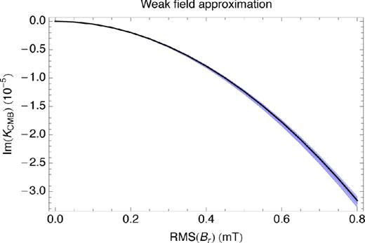
Im(KCMB) as a function of the rms of the total radial field |$\bar{B}_r$| in the weak-field approximation. The blue area shows results obtained for different randomly generated models of the magnetic field. The black line shows the result obtained from the approximate expression (19). Magnetic diffusivities are fixed to ηf = ηs = 1.6 m2 s−1. All magnetic field models have a constant ratio of dipole to total rms strength of |$\bar{B}_r^d$|/|$\bar{B}_r = 0.3$|.
Interestingly, if we compute |$K_b^c$| from eq. (15a) by using |$B_r = \sqrt{3}\bar{B}_r^d\cos \theta +\bar{B}_r^u$|, that is, a Br field comprised of an axial dipole (of rms strength |$\bar{B}_r^d$|) and a uniform part (of rms strength |$\bar{B}_r^u$|), we retrieve the same result as eq. (19) with |$\bar{B}_r^{nd}=\bar{B}_r^u$|. These results confirm that, in the weak-field limit, the contribution to the torque from all the non-dipolar components of the field is equal to the contribution that a uniform radial field with the same rms strength would have.
3 EFFECT OF THE MORPHOLOGY OF THE MAGNETIC FIELD ON THE EM TORQUE
In order to assess the importance of the morphology of the field on the EM torque in the general strong-field regime, we compare the torques obtained from different magnetic field models with the same rms strength. First, in Section 3.1, we consider the simple case of magnetic fields that are comprised of a single harmonic. This allows us to determine the relative contribution of each harmonic to the torque. Then, Section 3.2 is devoted to the general case of multiharmonic fields, which are obviously a more realistic configuration for the Earth's magnetic field. In Section 3.3 we assess the validity of approximating all non-dipolar components of the field by a uniform field. Sections 3.1–3.3 are concerned with |$K_b^c$|, the part of the coupling constant that is independent of time. Contributions from the time-variable modulation |$K_b^{{\rm mod}}$| are discussed in Section 3.4.
3.1 Single-harmonic magnetic fields
To focus on the effect of the field morphology, we fixed the electrical conductivities at 5 × 10⁵ S m−1 leading to magnetic diffusivities ηf = ηs = 1.6 m2 s−1. (The dependence of the torque on the electrical conductivities will be further discussed in Section 4.) Parameter γb appearing in eq. (9) is computed at the CMB (resp. ICB) for the case |$\bar{B}_r=0.5$| mT (resp. 4 mT).
Fig. 2 shows the real and imaginary parts of Kb for different values of l and m. Perhaps the most striking feature of Fig. 2 is the fact that, for l > 2, |$K_b^c$| is virtually independent of l. This indicates that, for a more complex field, the way the energy is partitioned among the different harmonic degrees (i.e. the power spectrum) should not be of crucial importance to the EM torque. The torque depends more significantly on the order m of the field, in particular the real part of |$K_b^c$|. This suggests that, for multiharmonic fields, the way the energy is partitioned among the different orders is likely to affect the amplitude of the resulting torque.
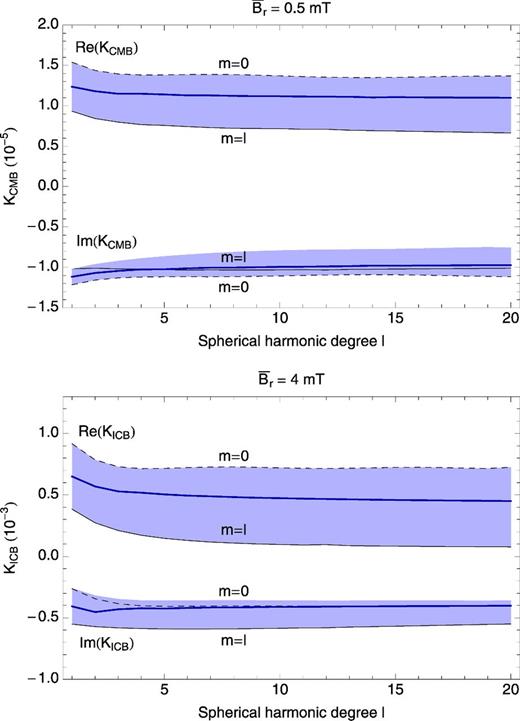
Coupling constants for magnetic fields comprised of a single harmonic (see eq. 20) as a function of the harmonic degree l and for different orders m. For every degree l, values for all the orders m are comprised within the blue shaded areas. Dashed (resp. solid) black lines show results for m = 0 (resp. m = l). The dark blue lines represent the average over all orders m for every degree l.
By comparing the results obtained for |$\bar{B}_r=0.5$| mT and |$\bar{B}_r=4$| mT, we confirm the idea that the effect of the field morphology is more important for a stronger field. Another difference between these two cases is the relative importance of the orders of the field, at least for Im(Kb). Indeed, for |$\bar{B}_r=0.5$| mT, orders m = 0 and m = l have almost the same value of Im(Kb) while for |$\bar{B}_r=4$| mT, the torque for m = l is significantly larger than that for m = 0. Note also that, for |$\bar{B}_r=0.5$| mT, Re(Kb) and Im(Kb) are approximately equal and opposite, as we expect in the weak-field approximation because of the factor (1 − i) in eq. (18). This symmetry no longer applies for strong fields.
3.2 Multiharmonics magnetic fields
We now turn to the more general case of a magnetic field model comprised of many harmonics. We generate models of the radial magnetic field based on the general form of eq. (1). In this section, we want to set the stage for testing the validity of approximating all non-dipolar harmonics of the field by a uniform field for the purpose of computing the EM torque. Thus, we remove the axial dipole part of the field and set cB10 = 0. Magnetic fields with a dipolar component will be considered in Section 4.
In order to test the importance of the power spectrum of the field on the strength of the EM torque, we consider four different cases represented on Fig. 3: (a) a flat power spectrum; (b) and (c) two log-linearly decreasing power spectra with different slopes and (d) a log-linearly decreasing spectrum for the first 14 degrees, followed by a uniform spectrum for larger degrees, with a jump in power between degrees 14 and 15. The reason for considering spectrum (d) will be given in Section 4.2.
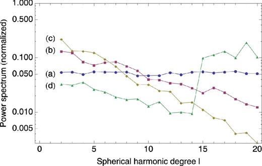
Realization of four different power spectra considered for the simulation of radial magnetic fields. (a) is a flat power spectrum, (b) and (c) are log-linearly decreasing and (d) is log-linearly decreasing up to degree 14 and then flat from degree 15, with a large jump between degrees 14 and 15. All the spectra are normalized such that |$\bar{B}_r=1$|.
To test the dependence of the torque on the way the energy is distributed between harmonics orders m, for each spectrum, we consider three different partitions: (1) a field with the energy equally partitioned (on average) between the orders, (2) a purely axisymmetric field, for which all the power is concentrated in the order m = 0 and (3) a strongly non-axisymmetric field, for which all the power is concentrated in the order m = l.
We then produce a suite of 30 different magnetic field models for each combination of spectrum and partition. First, for each individual field model, we add a random noise from a normal distribution with zero mean to the power spectrum. An example of the resulting power spectra with noise added is shown in Fig. 3. For the purely axisymmetric partition case, since there in only one non-zero field coefficient per degree, the amplitudes of the coefficients cBl0 are then set to match the power spectrum. The strongly non-axisymmetric field partition is dealt with similarly, except that there are two non-zero coefficients per degree (cBll, sBll) whose amplitude are chosen randomly on the interval [−1, 1] and then normalized such that the power at each degree l matches that prescribed by the power spectrum. For the equal partition of the energy among the orders, all the coefficients cBlm and sBlm are chosen randomly and independently from a uniform distribution on the interval [−1, 1]. We then normalize the amplitude of each of these coefficients such that the power at each degree l matches that prescribed by the power spectrum. Because the distributions are uniform, on average, there is equal power in all the different orders of the field.
Results are presented on Fig. 4. For each spectrum type, each dot corresponds to a given realization of the spectrum and, in the case of equal partition, to a given realization of the coefficients cBlm and sBlm. As in Section 3.1, we show results for both KCMB and KICB for magnetic field strengths of 0.5 mT and 4 mT, respectively.
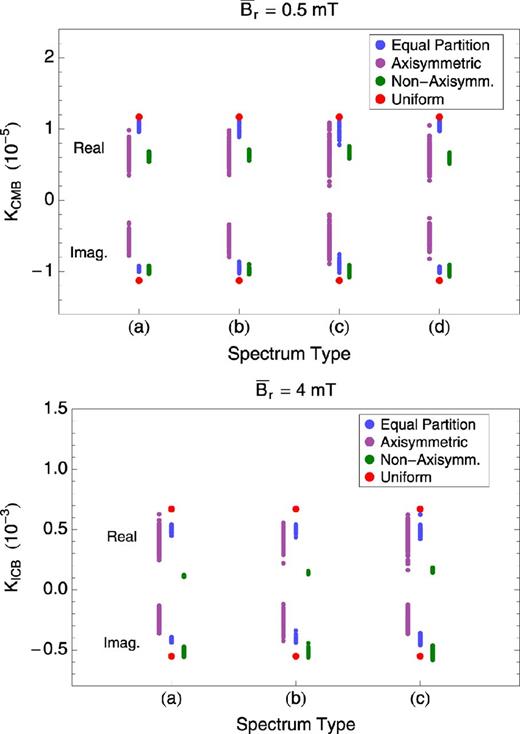
KCMB and KICB computed for different spectrum types (a, b, c, d) and three different partitions of the energy among the orders of the field: equal partition (blue), axisymmetric field (purple), strongly non-axisymmetric field (green). The rms strength is fixed to |$\bar{B}_r = 0.5$| mT for KCMB and to |$\bar{B}_r = 4$| mT for KICB. Red dots indicate the result obtained from a uniform radial magnetic field.
Fig. 4 illustrates that the results are virtually identical for all of the four spectra considered, while we observe large differences between results obtained for different partitions of the energy among the orders. Thus, this confirms the idea, already suggested in Section 3.1, that the EM torque is independent of the power spectrum of the field while it is very sensitive to the way the energy is partitioned among the harmonic orders of the field.
It is interesting to compare Fig. 4 to Fig. 2. The results obtained in the case of equal partition can be easily understood on the basis of the single-harmonic results. Indeed, in this case |$K_b^c$| is approximately equal to the average of the individual contribution from every single harmonic (represented by the blue line on Fig. 2). For highly non-axisymmetric fields, the results obtained are also close to those obtained for the individual harmonics with m = l (black solid lines on Fig. 2). The case of purely axisymmetric fields is more surprising: Fig. 4 indicates that Kb takes on values that are widely spread and much smaller than the values obtained for single-harmonic axisymmetric fields (black dashed lines on Fig. 2). In fact, the |$K_b^c$| values in Fig. 4 mostly lie outside of the blue shaded areas on Fig. 2. This suggests that, in strong field, axisymmetric field components interact with each others in their contribution to the total EM torque.
3.3 Validity of the uniform-field approximation
Our field models with equal energy partition mimic realistic non-dipolar magnetic field morphologies at the core boundaries. We now compare the torque from these models to the torque obtained from a uniform field of equivalent rms strength (red dots on Fig. 4). As Fig. 4 shows, the approximation of the non-dipolar field by a uniform field overestimates both Re(Kb) and |Im(Kb)|. At the CMB, for field strengths of the order of 0.5 mT, the uniform-field approximation overestimates |$K_b^c$| by about 15 per cent. The approximation by a uniform field may be deemed reasonable, though not perfect. This is not surprising as field strengths of 0.5 mT are not much larger than field strengths at which the weak-field approximation is valid. However, at the ICB, for field strengths of the order of 4 mT, the uniform-field approximation results in a poor estimate of the torque: it strongly overestimates the torque, by a factor as large as 30–40 per cent, and may thus be deemed invalid.
3.4 Time-variable modulation of the EM torque
We have shown in Section 2.3 that the coupling constant, or equivalently the EM torque, has a time-dependent contribution |$K_b^{{\rm mod}}$| that is given by eq. (10). For axisymmetric fields, namely with Br independent of φ, the surface integral in eq. (10) vanishes and thus |$K_b^{{\rm mod}}=0$|. As Buffett et al. (2002) considered the case of dipolar and uniform fields only, which are axisymmetric fields, this time-variable contribution was not taken into account. Here, because we deal with general magnetic field geometries which are not axisymmetric, we also have to consider this contribution.
As in Section 3.2, we generate magnetic field models from randomly generated Gauss coefficients. We used the power spectra illustrated on Fig. 3 and assume that on average, the energy is equally partitioned between the different orders of the field. We compute |$K_b^{{\rm mod}}$| at both the CMB and the ICB for magnetic field strengths of 0.5 mT and 4 mT, respectively. For all our simulated magnetic fields, |$K_b^{{\rm mod}}$| is smaller than |$K_b^c$| by at least a factor of 10. This indicates that, to a very good degree of approximation, Kb can be considered as constant in time. This approximation has been used in nutation models (Mathews et al.2002) and our results here justify this assumption on a more quantitative basis.
4 CONSTRAINTS ON THE MAGNETIC FIELD AT THE CORE BOUNDARIES
Observations of the Earth's nutations allow us to estimate the strength of the coupling at both the CMB and the ICB. These estimates are presented in Section 4.1. Different physical mechanisms can be responsible for the observed coupling, although observations require a mechanism that induces energy dissipation. If we assume that EM torque is responsible for the observed dissipative coupling, estimates of Kb can be used to constrain physical parameters involved in the EM torque, basically the electrical conductivities on the fluid and solid sides of the boundaries and the local radial magnetic field. Such constraints have been obtained previously, using the EM coupling model of Buffett et al. (2002) and the approximation of the non-dipolar components of the field by a uniform field (Mathews et al.2002; Koot et al.2010). However, as we have shown that the approximation of a uniform field is not valid at least at the ICB, we are motivated to reestimate these physical parameters on the basis of more realistic field morphologies. Section 4.2 is concerned with the constraints on the CMB while in Section 4.3 we consider the ICB.
4.1 Observational constraints
4.2 CMB
In order to model the EM torque at the CMB, we use the Gauss coefficients of the magnetic field model CHAOS-2s (Olsen et al.2009) for the first 14 harmonic degrees of the field. These coefficients vary in time over timescales of decades and longer. Nutation observations cover the time period from 1980 to 2012. As variations of the field during this period are too small to affect significantly the EM torque, we assume that the field is constant and take 2005 as the reference year.
If we compute the EM torque from these first 14 degrees, we get: KCMB = (0.55 − i 0.51) × 10−5, for σm = σf = 5 × 10⁵ S m−1. Compared to the observational constraint (21a), it is clear that the large-scale field at the CMB is not enough to explain the observed coupling constant at the CMB. Therefore, we also need to take into account the small-scale field that cannot be observed at the surface.
In order to do this, we simulate Gauss coefficients for harmonic degrees larger than 14. The power spectrum for these degrees is unknown but, as we have shown in Section 3.2, the details of the spectrum do not affect the EM torque. This gives us the freedom to choose arbitrarily the spectrum of the short-wavelength components of the field. A realistic power spectrum at the CMB is likely to have significant energy up to degree 100 or even larger (e.g. Buffett & Christensen 2007). Numerically, computing the EM torque for magnetic fields with at least 100 harmonic degrees leads to time-consuming integrals to solve. To speed up computations, we choose a spectrum truncated at degree L = 25. In order to reach large values for the field strength, we choose a power spectrum with a jump between degrees 14 and 15 as represented by spectrum (d) on Fig. 3. The first 14 degrees are from CHAOS-2s and the 11 larger degrees follow a flat spectrum (with an arbitrary random noise added).
It is important to specify the choice of partition of the energy among the orders of the field, as we have shown that this choice has a significant impact on the torque. Here, we make the hypothesis that, for the short-wavelength field, the energy is equally partitioned among the different orders and we simulate the Gauss coefficients in the way described in Section 3.2. This hypothesis seems to be reasonable given that for degrees 2–14, the energy is well partitioned between the orders.
Fig. 5 shows the results obtained for Im(KCMB) as a function of the rms strength of the field for σm = σf = 5 × 10⁵ S m−1. The smallest rms strength shown on Fig. 5 corresponds to the strength of the first 14 degrees of CHAOS-2s at the CMB, namely |$\bar{B}_r = 0.33$| mT. The blue shaded area shows the results obtained for different random realizations of the small-scale field. Also shown on Fig. 5 is the EM torque computed using the assumption that the radial field at the CMB is comprised of a dipole component (with g10 given by the CHAOS-2s field model) and a uniform component. As was already shown in Section 3.2, this approximation overestimates the torque by about 20 per cent.
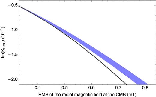
Im(KCMB) as a function of the rms strength of the radial magnetic field at the CMB. The blue shaded area shows the results obtained for different random realizations of the unknown small-scale field. The torque obtained from the approximation of the field by a dipole and a uniform components is shown by the grey line.
Fig. 5 indicates that the torques obtained for different realizations of the small-scale field are very similar (namely, the blue area is quite narrow). Therefore, the precise morphology of the unknown small-scale field at the CMB has only a little influence on the magnitude of the EM torque; the most important parameter is the rms strength of the field. Conversely, it is the rms strength of the field that can be potentially retrieved from nutation observations.
In order to derive further constraints on the CMB, we compute the coupling constant Im(KCMB) for different field extrapolations, as presented before, but also for different values of the electrical conductivities. Results are represented on Fig. 6 where different coloured areas show the results obtained from different choices of electrical conductivities.
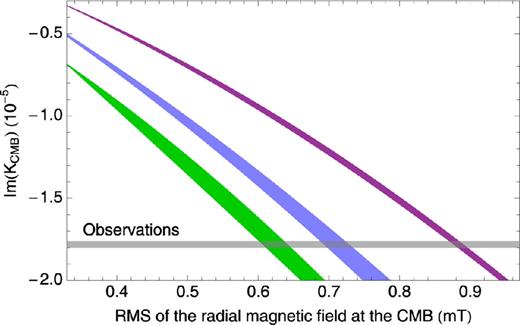
Im(KCMB) as a function of the rms strength of the radial magnetic field at the CMB for different realizations of the unknown small-scale field and different values of the electrical conductivities on both sides of the boundary: σm = σf = 5 × 10⁵ S m−1 (blue), σm = σf = 1.1 × 10⁶ S m−1 (green) and σf = 1.1 × 10⁶ S m−1, σm = 0.9 × 10⁵ S m−1 (purple). The grey area shows the observational constraint from nutation observations.
We note on Fig. 6 that the lower the electrical conductivities, the less important the effect of the small-scale field geometry is (shaded areas are thinner). This is because lower electrical conductivities give rise to smaller values of the parameter x± defined in eq. (13) and thus the EM coupling is closer to the weak-field limit for which the geometry effect is negligible. Also, for smaller values of x±, the dependence of Kb on |$\bar{B}_r$| is closer to quadratic than for larger values of x± for which the dependence tends more towards a linear behaviour. This can be easily understood from eqs (15a) and (17).
It is clear from Fig. 6 that the unknown spatial distribution of the small-scale field at the CMB (degrees larger than 14) does not limit significantly our ability to constrain the rms strength of the field. Indeed, this unknown field morphology introduces an uncertainty of the order of ∼0.03 mT (for σm = σf = 1.1 × 10⁶ S m−1) or less on the estimated |$\bar{B}_r$|. The largest uncertainty on |$\bar{B}_r$| is, by far, our poor knowledge of the electrical conductivities on both sides of the CMB.
Independent constraints on the field strength at the CMB and on the electrical conductivities cannot be retrieved as they both contribute to the strength of the EM torque. However, nutation observations favour a very high electrical conductivity at the base of the mantle (typically of the same order of magnitude as that of the core) because for lower values, the magnetic field required to explain the observations is very large, as shown in Fig. 6. A field of rms strength much larger than a few tenths of millitesla is not favoured because, in this case, the total Ohmic heating of the core could be larger than the power available to drive the geodynamo (Buffett & Christensen 2007). If we take the upper bound values for the electrical conductivity of both the outer core and lowermost mantle, namely σf = σm = 1.1 × 10⁶ S m−1, we can get a lower bound on the rms strength of the radial field at the CMB, of the order of ∼0.6 mT. If we take the conductivity of metallic FeO as an upper limit on the mantle side, σm = 0.9 × 10⁵ S m−1 (Ohta et al.2012), then the lower bound on the rms strength of the radial field at the CMB must be of the order of ∼0.9 mT.
4.3 ICB
As the power spectrum of the field does not affect the resulting EM torque (see Section 3.2), we arbitrarily choose the spectrum at the ICB to be flat, with degrees up to L = 20. Also, we make the assumption that, for degrees higher than 2, the energy is equally partitioned among the different orders of the field. The dipole component is a particular feature of the Earth's magnetic field: both at the surface and at the CMB, it dominates the power spectrum of the field. Therefore, at the ICB, where the importance of the dipole component is mostly unknown, we consider two distinct cases: a strongly dipolar field with |$\bar{B}_r^d/\bar{B}_r=0.8$| and a weakly dipolar field with |$\bar{B}_r^d/\bar{B}_r=0.3$|. For each set of Gauss coefficients, we vary the rms strength of the total field between |$\bar{B}_r=2$| mT and |$\bar{B}_r=16$| mT. We chose two different values of electrical conductivities on both sides of the ICB, namely 5 × 10⁵ S m−1 and 1.3 × 10⁶ S m−1, but, as expected, the results are independent of this choice. Results are shown on Fig. 7. Note the linear dependence of Kb on |$\bar{B}_r$| as was shown by the strong-field limit of eq. (17).
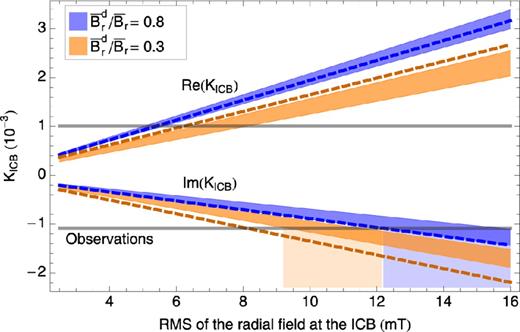
Coupling constant KICB as a function of the rms strength of the field at the ICB. Blue (resp. orange) areas are for the spectrum with |$\bar{B}_r^d/\bar{B}_r=0.8$| (resp. 0.3). Dashed lines show the results obtained from the approximation of the field by a dipolar and uniform component with the same rms. Grey horizontal lines indicate the observational constraints. Light blue and orange rectangles indicate the range of |$\bar{B}_r$| that matches the observational constraint on Im(KICB).
Fig. 7 also shows the results obtained for an approximation of the field by dipolar and uniform components. In the case of a strongly dipolar field, this approximation gives results that are not too different from those obtained from realistic field geometries because the contribution from the dipole largely dominates. Still, realistic field configurations introduce a significant spread in the possible amplitude of the torque that is not taken into account in the dipolar-uniform approximation. More importantly, for weakly dipolar fields, the dipolar-uniform approximation largely overestimates both Re(KICB) and |Im(KICB)|. This is consistent with our results of Section 3.3 for non-dipolar fields.
In order to get constraints on the properties of the ICB, we first consider those based on the observation of Im(KICB). Fig. 7 shows the values of |$\bar{B}_r$| satisfying the observed Im(KICB), both for the weakly and strongly dipolar fields. The weakly dipolar field requires |$\bar{B}_r$| to be between ∼9 and 12 mT and the strongly dipolar field requires |$\bar{B}_r$| to be between ∼12 and 16 mT. Clearly, the unknown morphology of the magnetic field induces a large uncertainty on the estimate of |$\bar{B}_r$|, of the order of a few milliteslas if the ratio |$\bar{B}_r^d/\bar{B}_r$| is known and even much higher if this ratio is unknown.
Moreover, we see that taking into account a more realistic morphology of the field leads to values of the estimated |$\bar{B}_r$| that are significantly larger than those obtained from the dipole-uniform field approximation used in previous studies. Indeed, with this approximation, the weakly dipolar field would require a strength of 8 mT while the strongly dipolar field implies a strength of 12 mT.
If we assume that all the observed dissipation is due to the EM coupling at the ICB, Fig. 7 indicates that this would require a magnetic field strength of at least ∼9 mT but possibly much higher. As for the constraint on Re(KICB), it requires a magnetic field at the ICB of at least ∼5 mT. Note, however, that no values of |$\bar{B}_r$| can explain both the observed Re(KICB) and Im(KICB) simultaneously, as was previously shown by Koot et al. (2010).
5 DISCUSSION AND CONCLUSION
EM coupling at the CMB and ICB depends on the local radial magnetic field as well as on the electrical conductivities on the fluid and solid sides of the boundaries. At the CMB, we have shown that the magnetic field affects the torque mainly through its rms strength, the unknown morphology of the small-scale field introducing only a relatively small uncertainty. The EM torque is also very sensitive to the electrical conductivities of the top of the core and bottom of the mantle. We thus confirm that, as was suggested by previous studies (Deleplace & Cardin 2006; Buffett & Christensen 2007), at the CMB, constraints on the rms strength of the field from nutation observations are mainly limited by the large uncertainties on the electrical conductivities, especially on the mantle side. The unknown morphology of the small-scale field introduces only a small uncertainty (of the order of 0.03 mT at most). Note, however, that if the field is approximated by a dipole and a uniform component, this leads to a larger error on |$\bar{B}_r$|, of the order of 0.1 mT for field strength of ∼0.7 mT.
For field strengths typical of the ICB, the situation is quite different. First, the EM torque is much less sensitive to the electrical conductivities, so that the uncertainties on these quantities do not affect significantly the results. Moreover, we have shown that the EM torque depends significantly on both the rms strength and the morphology of the field. Therefore, the unknown morphology of the field introduces a significant uncertainty on the EM torque at the ICB. In turn, this induces a large uncertainty on the constraints that we can get on |$\bar{B}_r$| from nutation observations.
The dissipation at the CMB observed in nutations suggests a very high value for the electrical conductivity on the mantle side of the CMB, thus supporting the idea of a metallic layer at the base of the mantle (Knittle & Jeanloz 1989; Ohta et al.2012; Otsuka & Karato 2012). An alternative possibility is that pockets of fluid core remain trapped by small wavelength topography of the CMB and act like a high effective mantle conductivity (Buffett 2010b). Although the conductivity required to explain the observations is clearly very high, it is important to keep in mind that the thickness of the conductive layer that is required is very thin, of the order of a few hundred metres. Nutation observations also require an rms strength of the radial field of at least ∼0.6 mT. This value is significantly higher than the rms of the first 14 degrees of the field, implying that a significant part of the energy of the field should be contained in the small-scale components that are not observable at the surface. These results are similar to those obtained in previous studies (e.g. Buffett 1992; Buffett et al.2002; Mathews et al.2002; Koot et al.2010).
At the ICB, our estimate of the rms strength of the field (between ∼9 and 12 mT for weakly dipolar fields and larger for fields with a stronger dipole component) is much larger than results obtained from the dipolar and uniform approximation which suggests a field strength of ∼8 mT (for weakly dipolar fields), when only the constraint from Im(KICB) is used. Recent estimates derived from fast torsional oscillations (Gillet et al.2010) and geodynamo models (e.g. Christensen & Aubert 2006) suggest field strengths of approximately 2–4 mT deep inside the core. Compared to these, the values obtained from nutation observations, and in particular the new values obtained here taking the field morphology into account, are much larger. Therefore, our results suggest that the dissipation observed at the ICB from nutations cannot be explained only by the EM coupling at the ICB, as we have assumed here. There should be at least one additional mechanism that contributes to energy dissipation. Two such mechanisms have already been proposed to explain (part of) the observed dissipation at the ICB: Ohmic dissipation in the outer core (Buffett 2010a) and viscous deformation of the inner core (Koot & Dumberry 2011). The results of our study thus reinforce the need for such an alternative mechanism to explain the dissipation observed in nutations.
L. Koot is supported by a post-doctoral fellowship from the National Fund for Scientific Research (FNRS), Belgium. M. Dumberry is supported by a Discovery Grant from NSERC/CRSNG.
REFERENCES
APPENDIX A: ROLE OF THE MAGNETIC FIELD GEOMETRY IN THE WEAK-FIELD LIMIT
The integral in eq. (15b) can also be solved analytically to get an expression of |$K_b^{{\rm mod}}$| in terms of field coefficients. The exact expression is more complicated than eq. (A1) and we do not write it here. The important feature is that it only includes terms that involve products of the form |${_{c,s}}B_{l\,m} \, {_{c,s}}B_{l^{\prime }\,m^{\prime }}$|, where either |$l\not=l^{\prime }$| or |$m\not=m^{\prime }$| or both. Thus, as is the case for the second term of eq. (A1), these terms tend to cancel out in the sum so that their contribution is negligible with respect to the constant term |$K_b^c$|.
