


Abstract
Nowadays, an increasing number of seismological imaging studies are published taking advantage of the increasing popularity of analysing empirical Green's functions obtained from high-frequency ambient seismic noise. However, especially on a local scale results could potentially be biased in regions where topography is not small compared to the wavelength and the penetration depth of the considered waves. Current 2-D seismic techniques are often inadequate when solving such 3-D geophysical problems, which include the complication of seismic imaging for cases where there are pronounced relief effects. For example, information about the geologic subsurface structure and deformational patterns is necessary for accurate site characterization and seismic hazard assessment. Here we show that an ad hoc passive seismic tomography approach can identify and describe complex 3-D structures, which can help to accurately and efficiently map the shear-wave velocities of the surficial soil layers, even in cases of significant topography relief. We test our technique by using simulations of seismic noise for a simple realistic site and show for a real data set across the Issyk-Ata fault, Kyrgyzstan, which is located at southern border of the capital, Bishkek, this novel approach has identified two different small fault branches and a clear shear-wave velocity contrast across the fault.
1 INTRODUCTION
Characterization of the internal structure of fault zones is an essential prerequisite for understanding and predicting their mechanical and seismic properties. Large-displacement faults generally produce much wider zones of deformation than smaller offset features. This provides much more scope for developing a complex internal geometry, which in turn may lead to significant modifications of the properties of these discontinuities. For large fault zones, geological studies show that the principal fault slip zone is often localized along bimaterial interfaces that separate rock units with considerably different properties (Sengor et al.2005; Dor et al.2008; Mitchell et al.2011). Sharp velocity contrasts are likely to be observed across major faults, which are generally interpreted as lithological discontinuities (Michelini & McEvilly 1991; Amato et al.1992; Eberhart-Phillips & Michael 1993; O’Connell et al.2007). Notably, a lithology contrast in the earthquake source region can produce an ambiguity in inferred seismic moments, associated with the multiple available choices for the assumed rigidity (Ben-Zion 1989; Heaton & Heaton 1989). Ben-Zion & Shi (2005) suggested, based on simulations of dynamic ruptures with off-fault plastic yielding, that strongly asymmetric damage zones on opposing sides of a fault are the cumulative product of earthquake ruptures on bimaterial faults separating different elastic bodies. Ignoring the near-surface structural properties across a seismic fault can produce biases and errors in derived earthquake locations and other structural properties and distort seismic hazard assessment (McNally & McEvilly 1977; Oppenheimer et al.1988; Ben-Zion & Malin 1991).
The topic of active fault studies is not new: Since the pioneering work of Aki & Lee (1976) large scale 3-D imaging of the seismogenic upper crust has become an important tool for the investigation of the nature of active fault zones. The occurrence of the 1995 Great Hanshin earthquake exactly on the mapped Nojima Fault reconfirmed this idea, emphasizing the importance of active fault studies. Thus, precise mapping and imaging has become one of the key aspects in terms of the possible location of future surface ruptures and near-fault seismic hazard assessment. Over the last few years, our ability to identify active faults has improved significantly, but in the absence of drilling, surface-based geophysical methods are necessary for the proper identification of fault zones and for the exact characterization of their properties.
Nowadays, multiple observations of geophysical properties like seismic body wave velocities in and adjacent to fault zones offer the greatest hope of making inferences about the fault, but up to now their resolution has been limited, particularly precluding the imaging of small-scale near-surface features. Active seismic imaging profiles (refraction or wide-angle profiles) can be useful for imaging surficial subsurface structures with shallow dips such as low-angle faults (Mooney 1989); although, in contrast, vertical or almost vertical faults are difficult to be identified by such methods (Mooney & Brocher 1987).
Here we present a rapid procedure for the passive imaging of near-surface properties by a weighted 3-D inversion procedure that also works in case of complex 3-D S-wave velocity structures under pronounced topographic conditions. The presented method can offer a more comprehensive view of the subsurface, having a greater areal extent and greater depth than traditional methods such as trenching or drilling. The success of these passive applications is explained by the fact that these methods are based on surface waves, which are always present in the ambient seismic noise wave field because they are excited preferentially by superficial sources. These waves can easily be extracted because they dominate the Green's function between receivers located at the surface.
To extract the exact Green's function, perfect diffuseness of the illuminating field is required. However, the diffuseness of a field relies on the equipartition of energy, which corresponds to equal energies with the independent modes of vibration. In this case, the energies undergo conspicuous fluctuations as a function of depth within about one Rayleigh wavelength (Sánchez-Sesma et al.2008; Perton et al.2009). Statistical treatment can be applied to such random wavefields, in particular to long time-series of ambient seismic noise. Since the distribution of the ambient sources randomizes when averaged over longer times (not more than a few hours for frequencies higher than a few hertz) the stabilization of the normalized averaged correlation function suggests that the resulting illumination is totally or partially equipartitioned (Sánchez-Sesma et al.2011).
Important developments in methodology set this work apart from previous studies: The estimated traveltimes were inverted by a rapid one-step tomographic algorithm. We decided in favour of this approach to calculate a 3-D S-wave velocity model instantaneously, keeping in mind a future application to monitoring. Moreover, classical imaging techniques are based on a flat Earth surface, implicitly assuming that the waves travel perfectly horizontally and do not follow the topography. Although this approximation is likely to be true for small frequency waves with wavelengths much greater than the amplitude of topographic variations due to the rather small penetration depths and short wavelengths of anthropogenic ambient seismic noise, in the case of strong topographic relief, a failure to use the right path length between the individual stations will lead to strong biases towards too small velocities (Wang et al.2012). This emphasizes the necessity that the inversion algorithm must properly account for the effects of topography.
Hereunto, we will first give an outline of the calculation of Rayleigh wave phase velocities and a description of the 3-D inversion procedure. To validate the technique, a synthetic example is presented, including a detailed discussion on the resolution of the algorithm and on some of the problems that can be encountered in tomographic inversion. Finally, after describing the data collection for a real-world data set on the Issyk-Ata fault in Kyrgyzstan, we will show that this approach can identify near-surface features across this fault.
2 CALCULATION OF TRAVELTIMES
The calculation of the Rayleigh wave phase velocities is based on the frequency-domain SPAC technique of Aki (1957). Whereas the classical SPAC method is used to retrieve the shallow S-wave velocity structure below a small array by means of the inversion of surface wave dispersion curves and, therefore, assumes an (almost) 1-D velocity–depth profile it is clear that for non-homogeneous subsoil conditions, the method suffers a severe drawback. That is, if the situation is more complicated (as, for example, across a region with a large velocity contrast) the classical SPAC method will provide significant perturbations in the observed S-wave velocity structure (Foti et al.2011). On the other hand, one can expect that, similarly to what is obtained over regional scales, local heterogeneities will affect the noise propagation on a small scale along the ray path between the sensors, and hence can be retrieved by analysing the Green's function estimated by the cross-correlation of the signals recorded at two different stations (Brenguier et al.2007; Picozzi et al.2009). As shown by Tsai & Moschetti (2010), the exact equivalence between the cross-correlation and the SPAC allows the results from each of the independent fields to be used in the other.
For calculating the cross-correlation functions between the stations, we consider only the vertical component of the recordings, which are strongly dominated by Rayleigh waves. A second order Butterworth high-pass filter was applied to these data using a corner frequency of 0.9 Hz, aiming at removing high-amplitude low-frequency irregularities that tend to obscure noise signals. For each of the chosen frequencies and for all |${{n(n - 1)} {/2}}$| possible station pairs, where n is the number of stations, the data were one-bit normalized (Campillo & Paul 2003) and, finally, stacked together which, on average, improves the signal-to-noise ratio. Finally, the traveltimes between all stations were calculated from the estimated phase velocities using the known distances between the sensors.
3 THE INVERSION ALGORITHM
The estimated traveltimes for the individual frequencies were inverted by a rapid tomographic algorithm to calculate a 3-D S-wave velocity model similar to Pilz et al. (2012) but accounting for the topographic relief. Since the S-wave velocity is the dominant property of the fundamental mode of high-frequency Rayleigh waves, we perform inversions for a S-wave velocity model estimation while considering the observed velocities in the 3-D frequency-dependent tomography as being representative of Rayleigh wave phase velocities.
Starting from a homogeneous 3-D velocity model, an iterative procedure using singular value decomposition for minimizing the misfit between the observed and theoretical traveltimes is adopted (Picozzi et al.2009; Pilz et al.2012). Additionally, to reduce the risk of divergence and to stabilize the iteration process, an adaptive bi-weight estimation (Tukey 1974; Arai & Tokimatsu 2004), which is a type of maximum likelihood estimation, is applied.
In particular, the measured slowness along each ray path contains information about the underlying structure to depths corresponding to approximately one-third to one-half the wavelength of each frequency (Foti et al.2009). Since shallow blocks are sampled more intensely than deeper ones, we introduce a further constraint on the solution by adding a MNF × MNF weighting matrix K which weights the data depending on the number, length, orientation and vertical penetration depth of each ray path segment crossing each cell. According to Yanovskaya & Ditmar (1990), for the 3-D problem the weights in K turn out to be representable as a product of two functions, one depending on the horizontal properties, that is, the number, path length (in consideration of the relief, see explanation in the next paragraph) and orientation of the ray paths, and the other one depending on the vertical penetration depth, that is, the frequency of each ray path segment crossing each cell. Additional smoothness constraints are implemented by adding a system of equations to the original traveltime inversion problem, following Ammon & Vidale (1993) and Picozzi et al. (2009). Due to the rather small penetration depths and short wavelengths of ambient seismic noise, in the case of strong topographic relief, a failure to use the right path length in each of the cells will lead to incorrect weighting and therefore to biases towards too small velocities.
4 WEIGHTING SCHEME
For the horizontal weights, the singular values of the ray density matrix were used to calculate its ellipticity following Kissling (1988). If several rays with different azimuths cross the cell, the ellipticity is close to 1 and a good resolution for the cell is achieved. Therefore, the horizontal weights were computed by multiplying the ellipticity for the number of rays crossing each cell.
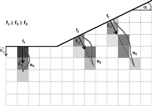
Calculation of the vertical weights for different frequencies for the block's cells, based on the displacement component u3 for Rayleigh waves. The darker the individual cell's colour, the higher the weight. Note that the weight is calculated perpendicular to the slope of topography.
5 SYNTHETIC TESTS
To ensure the reliability of the proposed technique, synthetic time-series of seismic noise were computed using a spectral element code, developed by the Center for Advanced Studies, Research and Development, in Sardinia and the Department of Structural Engineering of the Politecnico di Milano (Faccioli et al.1997). The underlying model consists of a block with two homogeneous layers characterized by different S-wave velocities with the intersecting plane of the two structures dipping at an angle of around 50°. The surface of the modelled block is characterized by a gradient with the slope angle changing where the two blocks emerge at the surface (Fig. 2). There is a shift of the velocity contrast towards the bottom of the slope at 18 m below the surface of the low-velocity block. Since only cultural noise higher than a few Hertz is considered, such synthetic wave fields can be modelled as a distribution of impulsive point forces located at the surface or subsurface of the studied medium, having random force orientation and amplitude (Lachet & Bard 1994). Such a random force was applied at each time step of 0.01 s at 200 different locations, arbitrarily distributed over an area covering the entire block's surface and a frame being 100 meters wide and surrounding the block. The noise sources are distributed isotropically around the area of interest guaranteeing a diffuse noise wave field.
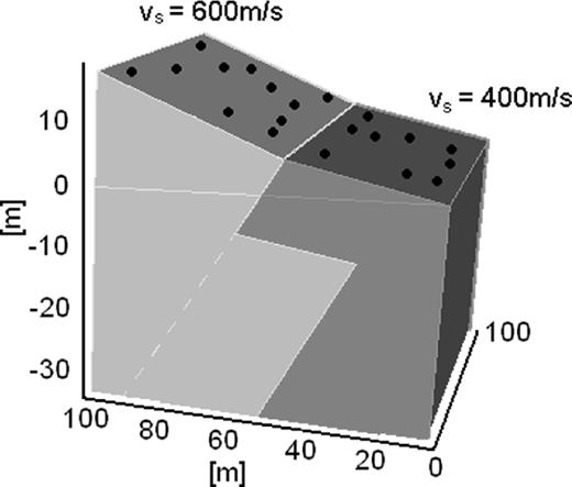
Simple 3-D structure used for the calculation of the noise synthetics. The two blocks are characterized by different shear-wave velocities. The black dots show the location of the receivers on the surface of the block.
From the continuous data sets recorded by 20 receivers, 60 noise windows of 30 s were extracted. Picozzi et al. (2009) have shown that this duration is sufficient for obtaining a reliable estimate of the Green's function between two sensors for distances of some tens of meters. After removing the linear trend from each window, a 5 per cent cosine taper was applied at both ends. For each frequency (5 Hz ≤ f ≤ 15 Hz at intervals of 1 Hz) the traveltime between each pair of receivers has been calculated and the final inversion has been carried out using five different frequency values (5, 6, 9, 12 and 15 Hz).
In Fig. 3, the inversion results giving the average S-wave velocities are shown. The comparison between the input structure and the calculated velocities shows that the structure is satisfactorily reproduced. The two blocks characterized by different S-wave velocities and their shift for deeper parts of the block can clearly be identified. The absolute S-wave velocities are fairly well reproduced. However, since a set of smoothing parameters has been introduced in the solution, there is no sharp contrast between the two blocks, but only a more gradual transition. Nonetheless, we offer a note of caution: Since the resolution of our imaging technique is expected to decrease with depth, thus the tomographic signature of the velocity contrasts becomes weaker with increasing depth. Eq. (4) further implies that the vertical weights vary smoothly, from which it follows that vertical discontinuities and S-wave velocity inversions (i.e. a cell having an S-wave velocity lower than the corresponding cell above) will be resolved less sharply.

6 RESOLUTION TESTS
A meaningful and reliable interpretation of tomographic results requires an accurate analysis of the solution quality with all available resolution tools. To this regard, checkerboard resolution tests were carried out to confirm that the major velocity features can be adequately resolved. Our 3-D checkerboard test consists of adding a regularly varying perturbation with the appearance of a 3-D checkerboard to the final velocity model derived from the tomographic inversion. Based on the checkerboard, traveltimes are then calculated through the perturbed model, and a random traveltime variation is added to simulate realistic arrival times. The random times are selected from Gaussian distributions whose half-widths are consistent with the standard error estimates for the individual traveltime data (maximum error 0.007 s). Resolvability at any point of the model space is defined in terms of the ratio of recovered velocity anomaly to the real velocity perturbation.
The comparison between synthetic and restored models (Fig. 4) shows that both the checkerboard structure and the simulated anomaly are satisfactorily reproduced. A clear checkerboard structure can be identified on the top for the central area of the synthetic model where the path coverage is dense, giving a further strong indication that, in well resolved areas, the estimates of the recovered velocity anomalies are robust. Only at the edges of the model the ray coverage is insufficient to resolve the local structure with full confidence. In this case, the regularization acts to smooth the model towards lateral homogeneity. For the deepest parts, there is only limited recovery of the checkerboard due to the large decrease in the density of the rays with bottoming points, indicating poorer lateral resolution at depth. The near-surface properties are well resolved down to a depth of around 40 m.
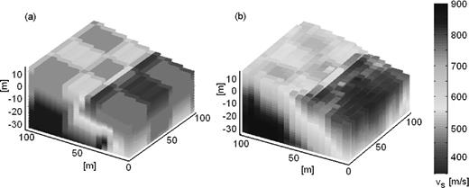
3-D tomography with checkerboard. (a) The perturbed velocity model, generated by adding 20 per cent perturbation for every 20 m of depth below the surface on the initial model shown in Fig. 2. (b) The reconstructed model from the 3-D tomography.
In Fig. 5 the resolution of the velocity model shown in Fig. 3 is displayed by the spread function. It is clear that where there is adequate resolution the velocity reasonably agrees with the values of the underlying model. Overall the resolution close to the surface is high, in particular for the left part of cross-section E in Fig. 5. Similar to the horizontal weights also the horizontal model resolution of a cell depends on the number of rays crossing the cell and their angular distribution, rather than by the presence of nearby receivers, meaning that also the edges of the block show relatively high resolution except for the central part of cross-section A in Fig. 5.
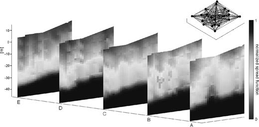
Horizontal cross-sections of the normalized spread function for the S-wave velocity model shown in Fig. 3. Black dots show location of sensors and black lines represent the ray paths.
There is a decrease in resolution with depth since fewer frequencies sample these parts of the block. The model can be well resolved down to a depth of around 35–40 m, being approximately one-third to one-half the wavelength of the lowest frequency. The depth might even be increased using more extended array configurations. Such depths cannot be reached by traditional methods such as trenching, pointing out the potential of the method for imaging near-surface structures.
7 THE ISSYK-ATA FAULT: CHARACTERISTICS AND DATA ACQUISITION
The studied natural example for obtaining images by means of real-world data is the Issyk-Ata fault in Kyrgyzstan, a moderately dipping thrust to reverse fault defining the northern deformation front for the central Tien Shan between ∼74°E and ∼75°E longitude (Fig. 6; Chediya et al.1998; Thompson et al.2002). Although the fault has not ruptured within the last 200 yr (and possibly longer) and has been believed to be seismically less active, traces of palaeoseismic deformations indicate that strong earthquakes have occurred in the past in this area and hence will probably occur again in the future (Abrakhmatov et al.2002; Landgraf et al.2012). A probabilistic assessment of the seismic hazard has recently been computed on a regional scale (Abrakhmatov et al.2003; Erdik et al.2005; Bindi et al.2011) showing that the highest hazard for the country of Kyrgyzstan lies along the southern border of the city of Bishkek, the country's capital with almost one million inhabitants, close to the Issyk-Ata fault system. Thompson et al. (2002) have estimated a Quaternary slip rate of 2.1 +1.7/−0.3 mm yr–1 for the central part of the fault.
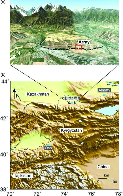
(a) Satellite image showing the southern outskirts of Bishkek facing the Ala-Too range. The topography is exaggerated by two times. Location of the array measurement is indicated. The dotted line shows the Issyk-Ata fault following Chediya et al. (2000). Google Earth, © 2012, CNS Spot Image © 2012, Digital Globe © 2012. (b) Map of Central Asia. Major faults are mapped in orange.
For our study, the data set is comprised of simultaneous recordings of seismic noise at 18 sites deployed in the Orto-Say district in southern Bishkek, spanning an area of 240 m × 160 m with the highest station being located around 20 m above the lowest and at the same time presumably crossing the surface appearance of the Issyk-Ata fault considering geological information (Chediya et al.2000). In fact, although the precise location of the fault is hardly known some studies (e.g. Korjenkov et al.2012) locate the fault near the base of the foothills limiting the Chuy basin to the south.
The array consisted of 14 Earth Data Logger (EDL) 24-bit acquisition systems equipped with 12 short-period Mark L4C-3D sensors, a Güralp CMG-ESPC 60 and a IO-3D 4.5 Hz sensor, and 4 Reftek 130 digitizers connected to Lennartz Le3D-5s seismometers. Seismic noise was recorded simultaneously by all stations for more than 2 hr on 2008 August 18 at a sampling rate of 500 samples s–1. The continuous data sets were divided into 240 windows of 30 s. Following the same course of action as described in the previous paragraphs the SPAC coefficients and the corresponding traveltimes between all stations in a frequency range of 3 Hz ≤ f ≤ 13 Hz at intervals of 1 Hz have been calculated. The frequency–wavenumber ( f–k) analysis carried out using the maximum likelihood method (Capon et al.1967) shows that the anthropogenic seismic noise sources in this frequency range are more scattered over the wavenumber plane, with the largest energy coming from a narrow azimuthal range in the north being around 90° wide, that is, from the city of Bishkek (not shown). Although such a non-uniform distribution of seismic noise sources might bias the reconstruction of attenuation of the studied media when one-bit normalization is used (Larose et al.2007) it will have only very minor influence on the phase, that is, on the calculation of the traveltimes, provided sufficiently long recording times in which enough energy is coming from the remaining azimuthal sectors (Derode et al.2003; Larose et al.2007; Yang & Ritzwoller 2008; Picozzi et al.2009; Yao & van der Hilst 2009). Even if all the noise sources are distributed in an even narrow range the velocity error will be in the order of a few percent (Cupillard & Capdeville 2010), which can be tolerated in engineering seismology. Using 120 min of recording, the estimated traveltimes were found to be stable and have been inverted by a tomographic approach using five different frequency values (4, 5, 7, 10 and 13 Hz).
8 TOMOGRAPHIC IMAGING RESULTS AND INTERPRETATION
The inversion results of the array recordings obtained after 500 iterations are shown in Fig. 7. A clear difference in S-wave velocity is observed, contrasting the northern and the southern parts of the studied area and running in an east-west direction parallel to the fault. Such a rather strong velocity contrast across the Issyk-Ata fault close to the surface is not a unique feature and has already been observed for other faults (Lewis et al.2007; Roux et al.2011). The transition zone is rather sharp, spanning only some tens of meters. On such small scales of up to 10 m, representing the internal fault zone structure, regularization of geometrical incompatibilities on the fault surface with progressive slip produces a tabular zone of granular rock that becomes fault gouge. Based on Ben-Zion & Sammis (2003) and Korjenkov et al. (2012) we interpret this sharp velocity contrast as such a consistent fault structure tending to evolve with cumulative slip towards geometrical simplicity.
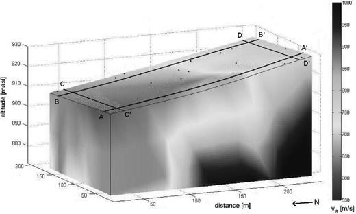
Inversion results of measurements on the Issyk-Ata fault obtained after 500 iterations. Topography is exaggerated about three times. The dots represent locations of the sensors. Locations of cross-sections shown in Fig. 8 are indicated by straight black lines.
A distinct low-velocity wedge in the uppermost part of the northern section of the studied area can be identified (reddish colour in Figs 8a and b) which might be caused by fault scarp weathering and present-day detritus which had slid off from the rock terrace. In this interpretation, formation of the colluvial wedge would represent multiple faulting events with a total displacement of around 10 m; this value is similar to the findings of Korjenkov et al. (2012) who carried out geological investigations around 1 km to the east of our study site.
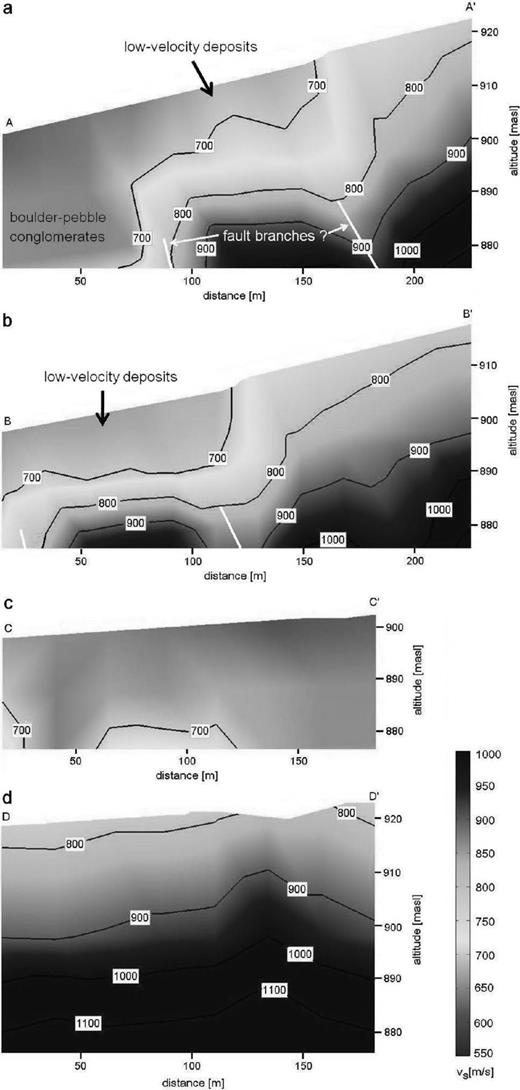
Cross-sections from the 3-D S-wave velocity model with (a) and (b) being north–south cross-sections and (c) and (d) being east–west cross-sections. For all profiles the topography is exaggerated about three times. Velocity isolines are mapped as thick black lines.
The estimated absolute S-wave velocities are robust and compatible with the findings of previous studies (Parolai et al.2010) for similar material in Bishkek. Below the low-velocity deposits the material can be interpreted as late Pleistocene and Holocene terraces of boulder-pebble conglomerates and alluvial fans that form the lower surface of the alluvium plain of the Chu basin (Korjenkov et al.2012). Of course, stratigraphy becomes more difficult to interpret northward due to the spatially and temporally discontinuous nature of deposition and erosion. On the contrary, Pliocene conglomerates with dense carbonate cement with gravel stones form the high velocity bluish part in the south (Korjenkov et al.2012, Figs 8a and b). Whereas such clear differences can be found in the north–south cross-sections and might be interpreted as shallow fault traces for both east–west cross-sections, on the contrary, the velocity and most probably also the material is rather homogeneous with no lateral discontinuities (Figs 8c and d).
The dip angle of the fault close to the surface is around 50°. Although the exact dipping cannot completely be recovered due to intrinsic vertical smearing of the inversion algorithm the detected value is in agreement with Bullen et al. (2001) who is reporting dip angles in the range of 45°–50°. This information is valuable for the calculation of Quaternary shortening (Bullen et al.2003) but it can also be used for the assessment of reliable seismic risk scenarios. It has been reported that the near-fault fault-normal peak velocities strongly depend on fault dip (e.g. Oglesby et al.2000) and that for dipping angles greater than ∼50° the maximum fault-normal peak velocities will appear on the footwall (O’Connell et al.2007), that is, north of the Issyk-Ata fault. Additionally, following Ma & Beroza (2008), the ground motion on the footwall might further be amplified due to the more compliant low velocity materials. Therefore, to obtain realistic estimates of ground motion it is therefore unavoidable to consider also the fault dip as well as the strong lateral velocity contrasts across the top several kilometres in ground motion prediction relations.
Two parallel fault structures can clearly be depicted (Figs 8a and b), one lowering the Tertiary by nearly 30 m, and the other lowering the top of the Tertiary strata to greater, but unresolved, depths to the north. Chediya et al. (2000) already found that the alluvial sequence in this fault zone can be disturbed by several thrusts that are generally concordant with the main fault. Also Korjenkov et al. (2012) elaborate the existence of such secondary splitting faults along the foothills in the same area. Such splitting effects could be the source of the high-frequency content of strong ground motion (Bhat et al.2007), exposing the city of Bishkek to a high level of hazard.
9 OUTLOOK AND CONCLUSIONS
Based on the correlation of seismic noise recordings, we have shown that with a limited number of seismic stations and recording times of several tens of minutes, detailed images of the local subsoil structure can be obtained even under pronounced topographic conditions. The reliability of the proposed technique and its resolution capacity were validated using synthetic data sets showing that the results are well constrained. The displayed images obtained by synthetic data and for a real-world example, the Issyk-Ata fault in Kyrgyzstan, which may act as a major contributor of earthquake ground motion and basin-generated wave field effects in the Chu basin and the city of Bishkek, can serve as a valuable example that such images can be obtained even in cases of significant topography relief. In contrast to information gained from traditional 2-D trench excavation, such pointwise seismic imaging can add an extra dimension and a deeper perspective. In particular, the depth of investigation might be enlarged using more extended array configurations. Our study demonstrates that useful results in terms of realistic velocity structures and geometries can be obtained even in complex environments whose geology and physical properties are hardly known.
The speed of the urban growth with an increase in Bishkek's population of almost 10 per cent in the last 10 yr (Abdykalykov et al.2009) is exposing more and more people and expanding infrastructures to seismic hazards. In combination with earthquake early warning and rapid response procedures for real-time risk assessment (Picozzi et al.2013), several similar arrays distributed along the fault can be used for precise monitoring. In particular, making use of low cost and wireless self-organizing seismic sensors can serve as an alternative and new technique without the need for a planned, centralized infrastructure (Picozzi et al.2010). The presented method can overcome shortcomings like poor spatial resolution which have been reported for other passive processing techniques in complex structures like volcanoes or fault zones (Sabra et al.2006; Sens-Schönfelder & Wegler 2006; Wegler & Sens-Schönfelder 2007; Hadziioannou et al.2009). While the classical SPAC equations have been derived for the analysis of the vertical component of ground motion they can in principle be adapted for the analysis of the horizontal components although the extraction of phase-velocity information for the single phases is not straightforward due to the superposition of both Rayleigh and Love waves (Boxberger et al.2011). Anyhow, since the presented method only uses the phase and not the amplitude information associated with the direct or scattered waves, the scattered part of the correlation functions is stable enough to provide robust velocity estimates with which changes in the medium properties can be monitored.
Therefore, the method is particularly advantageous since it can return useful information about the heterogeneous subsurface structure and structural changes therein in complex environments across seismic faults or areas prone to landslides almost in real time even if earthquakes do not occur. Although such information about the S-wave velocity distribution is difficult to acquire with traditional methods, simply analysing the ambient noise field by the means described here can serve as a reliable and economical alternative.
Research has been carried out under the project MIIC – Monitoring and Imaging by Interferometric Concepts founded by the German Ministry of Education and Research (BMBF Project 03G0736B). We are grateful to U. Abdybachaev, P. Augliera, E. D'Alema, S. Orunbaev, A. Strollo, J. Tokmulin and S. Usupaev for assistance during the field work. K. Fleming kindly revised our English. Instruments were provided by the Geophysical Instrumental Pool of the Helmholtz Center Potsdam.
