


Abstract
We develop and apply a full waveform inversion method that incorporates seismic data on a wide range of spatio-temporal scales, thereby constraining the details of both crustal and upper-mantle structure. This is intended to further our understanding of crust–mantle interactions that shape the nature of plate tectonics, and to be a step towards improved tomographic models of strongly scale-dependent earth properties, such as attenuation and anisotropy.
The inversion for detailed regional earth structure consistently embedded within a large-scale model requires locally refined numerical meshes that allow us to (1) model regional wave propagation at high frequencies, and (2) capture the inferred fine-scale heterogeneities. The smallest local grid spacing sets the upper bound of the largest possible time step used to iteratively advance the seismic wave field. This limitation leads to extreme computational costs in the presence of fine-scale structure, and it inhibits the construction of full waveform tomographic models that describe earth structure on multiple scales. To reduce computational requirements to a feasible level, we design a multigrid approach based on the decomposition of a multiscale earth model with widely varying grid spacings into a family of single-scale models where the grid spacing is approximately uniform. Each of the single-scale models contains a tractable number of grid points, which ensures computational efficiency. The multi-to-single-scale decomposition is the foundation of iterative, gradient-based optimization schemes that simultaneously and consistently invert data on all scales for one multi-scale model.
We demonstrate the applicability of our method in a full waveform inversion for Eurasia, with a special focus on Anatolia where coverage is particularly dense. Continental-scale structure is constrained by complete seismic waveforms in the 30–200 s period range. In addition to the well-known structural elements of the Eurasian mantle, our model reveals a variety of subtle features, such as the Armorican Massif, the Rhine Graben and the Massif Central. Anatolia is covered by waveforms with 8–200 s period, meaning that the details of both crustal and mantle structure are resolved consistently. The final model contains numerous previously undiscovered structures, including the extension-related updoming of lower-crustal material beneath the Menderes Massif in western Anatolia.
Furthermore, the final model for the Anatolian region confirms estimates of crustal depth from receiver function analysis, and it accurately explains cross-correlations of ambient seismic noise at 10 s period that have not been used in the tomographic inversion. This provides strong independent evidence that detailed 3-D structure is well resolved.
1 INTRODUCTION
Seismic tomography is our primary source of information on the current state and the evolution of the Earth’s interior from the local to the global scale. Since its conception and first applications in the 1960s and 1970s (e.g. Backus & Gilbert 1967, 1968, 1970; Aki & Lee 1976), it has branched into a large number of varieties, each targeted at specific aspects of earth structure. These varieties include different forms of traveltime tomography (e.g. Kissling 1988; Spakman et al.1993; Gorbatov & Kennett 2003; Lebedev & van der Hilst 2008; Tian et al.2009), surface wave tomography (e.g. Yoshizawa & Kennett 2004; Fishwick et al.2005; Zhou et al.2006; Nettles & Dziewoński 2008), normal-mode inversions (e.g. Giardini et al.1987; Deuss 2008) and combinations thereof (e.g. Ritsema et al.1999; Panning & Romanowicz 2006; Ritsema et al.2011). The numerous applications of seismic tomography have drawn the picture of a vigorously convecting planet, with large-scale up- and downwellings consistently imaged as isotropic velocity perturbations. Comprehensive summaries of these results can be found in numerous recent reviews (e.g. Rawlinson et al.2010; Liu & Gu 2012; Trampert & Fichtner 2013).
Despite substantial progress, at least two major challenges remain: (1) While there is comparatively broad consensus on 3-D isotropic earth structure, reproducible tomographies are still not available for strongly scale-dependent properties. These include Q and anisotropy, which are essential to infer temperature and deformation in the Earth. (2) The details of 3-D structure in the crust and the mantle cannot be resolved consistently and simultaneously. This results in a poor understanding of crust–mantle interactions that shape the nature of plate tectonics. We will elaborate on both challenges in the following paragraphs.
1.1 Scale-dependent properties of the Earth
Scale dependence results from limited resolution and the closely related need to regularize generally underdetermined tomographic inverse problems. Regularization prevents the appearance of small-scale artefacts by forcing solutions to be smooth. While having a comparatively minor effect on the characteristics of isotropic velocity variations, the enforced absence of small-scale structure produces apparent large-scale variations of scale-dependent properties. This effect is aggravated by the inherent subjectivity of regularization, thereby compromising both reproducibility and interpretations in terms of the Earth’s dynamics and thermochemical structure. Properties that are particularly affected by scale dependence are Q and anisotropy.
Viscoelastic dissipation in the Earth, typically parametrized in terms of Q or its inverse, is mostly inferred from the frequency-dependent amplitudes of seismic waves (e.g. Canas & Mitchell 1978; Flanagan & Wiens 1998; Kennett & Abdullah 2011). In addition to Q, amplitudes depend on the sharpness, that is the small-scale aspect, of purely elastic variations that lead to focusing and defocusing. However, sharpness is deliberately reduced by regularization, which contributes to the low correlation of global Q models that hardly exceeds 0.4 over length scales of 4000 km (Romanowicz 1995; Reid et al.2001; Selby & Woodhouse 2002; Warren & Shearer 2002; Gung & Romanowicz 2004; Dalton et al.2008). Further complication is added by the possibility to explain attenuation at high frequencies nearly equally well by either viscoelastic dissipation or scattering off purely elastic small-scale heterogeneities (Aki 1980a,b).
The scale dependence of anisotropy has been studied extensively (Riznichenko 1949; Backus 1962; Capdeville et al.2010a,b, 2013). Seismic waves do not distinguish between large-scale anisotropy and small-scale isotropic heterogeneities much smaller than a wavelength. Most radially anisotropic models of the Earth are indeed fully equivalent to finely layered and purely isotropic models (Fichtner et al.2012). The suppression of small-scale isotropic features, therefore, maps into large-scale apparent anisotropy. This problem acquires additional complexity through the strong spatial and directional dependence of tomographic resolution (Fichtner & Trampert 2011b), which leads to space- and direction-dependent smoothing. The results are apparent variations of anisotropy that are unrelated to intrinsic anisotropy in the Earth.
A small-scale feature with special relevance is the crust. Unavoidably inaccurate crustal models are a well-documented source of apparent anisotropy and a major obstacle in anisotropic tomography (Bozdağ & Trampert 2008; Ferreira et al.2010). Within the crust, numerical modelling of coda waves provides evidence for a nearly self-similar distribution of heterogeneities across a wide range of length scales (Frankel 1989). For the mantle, indicators for the existence of small-scale heterogeneities come from various sources. Stochastic heterogeneities with correlation lengths at the kilometre-scale explain the propagation of high-frequency waves through lithospheric material (Furumura & Kennett 2005; Kennett & Furumura 2008) and seismic profiles from nuclear explosions (e.g. Morozova et al.1999; Rydberg et al.2000). Receiver functions suggest the presence of a mille-feuille structure with elongate melt pockets in the asthenosphere beneath oceans (Kawakatsu et al.2009). Based on observations of PKP precursors, Hedlin et al. (1997) suggest the presence of ∼10-km-scale heterogeneities throughout the mantle. From a geodynamic perspective, convection in the Earth at high Rayleigh and low Reynolds number may lead to a regime where mantle material is well stirred, but where initially distinct components are not well mixed (e.g. Davies 1999). Heterogeneity will thus become streaky, with small-scale variations in some directions.
1.2 Simultaneously resolving crustal and mantle structure
Most studies of earth structure consider either the crust or the mantle. This requires assumptions on one of the two, which can lead to artefacts in the inferred structural properties.
This contamination effect is best studied in surface wave tomography for mantle structure. Surface waves at periods above ∼30 s are sensitive to crustal structure, without being able to resolve it. Since wave propagation through the strongly heterogeneous crust is difficult to model, crustal corrections are typically applied to surface wave data (e.g. Woodhouse & Dziewoński 1984; Marone & Romanowicz 2007; Lekić et al.2010). These corrections rely on crustal models (e.g. Crust2.0 (Bassin et al.2000) or 3SMAC (Nataf & Ricard 1996)) that are poorly constrained in some regions. The inaccuracies of the assumed crust map into incorrect mantle structure, and into artificial anisotropy in particular (Bozdağ & Trampert 2008; Ferreira et al.2010).
Similarly, crustal studies are affected by the inaccuracies of mantle structure. Receiver functions, for instance, depend on the incidence angle of body waves, which is influenced by 3-D mantle heterogeneity. When not accounted for, mantle structure can lead to an apparent azimuthal dependence of receiver functions. This translates into an artificial blurring of receiver function stacks and a smoothing of the inferred discontinuities. The azimuthal dependence itself may be misinterpreted as irregular topography on discontinuities.
Both challenges—scale dependence and simultaneous crust–mantle resolution—are closely related. Small-scale structure is not included in a priori models of the crust, used for crustal corrections in mantle tomography. This produces artefacts in the inferred mantle models, especially in its strongly scale-dependent properties.
1.3 Problem statement
While limited data coverage and dissipation in the Earth withhold much of the information necessary to fully resolve small-scale structure in both crust and mantle, there are feasible improvements that can lead to more reliable and detailed tomographic models:
Seismic wave propagation through the strongly heterogeneous crust should be modelled and inverted on the basis of fully numerical techniques. They ensure that the complete seismic wavefield can be simulated accurately, without the need for crustal corrections.
Complete seismograms rather than isolated seismic phases should be exploited for the benefit of improved resolution. Incorporating scattered waves, for instance, constrains sharp interfaces that are poorly visible in the direct body and surface waves (Stich et al.2009; Danecek et al.2011). Using as much information from seismograms as possible is particularly important in regions with low data coverage.
Local and regional seismic data at higher frequencies should be incorporated into larger-scale tomographies in order to improve the two most important resolution-controlling factors: frequency and geographic coverage. This will lead to stronger constraints on the details of shallow structure, and to more reliable images of scale-dependent properties in the mantle.
A large variety of numerical wave propagation methods have been developed in recent years (e.g. Moczo et al.2002; Dumbser et al.2007; Peter et al.2011; Cupillard et al.2012). They can be combined with adjoint techniques (e.g. Tarantola 1988; Tromp et al.2005; Fichtner et al.2006; Plessix 2006; Liu & Tromp 2008; Chen 2011) into full waveform inversion schemes that can exploit complete seismograms, including all types of body, surface and scattered waves (e.g. Bamberger et al.1982; Chen et al.2007; Fichtner et al.2010; Tape et al.2010; Rickers et al.2012; Zhu et al.2012; Rickers et al.2013). This means that items (1) and (2) in the previous list can already be addressed today.
The combination of data sets on multiple spatial scales has become almost a standard in tomographic inversions based on ray theory (e.g. Bijwaard et al.1998; Lebedev & van der Hilst 2008; Schäfer et al.2011). The inversion grid is adapted to the spatially variable resolution to represent smaller-scale structure and to prevent the appearance of artefacts in poorly covered regions. This type of multiscale tomography provides a more complete picture of earth structure but is limited by the validity range of ray theory that cannot handle the strong heterogeneities typically found in the lithosphere.
Numerical wave propagation overcomes this limitation of ray theory, and it provides accurate solutions for earth models with fine-scale heterogeneities. In regions where sufficient data are available to constrain small details, the numerical mesh must be refined for two reasons: First, because we need to model waves with high frequencies to constrain detailed structure, and secondly, because small-scale structure must be sampled sufficiently to produce accurate numerical solutions. This is schematically illustrated in Fig. 1. In time-domain numerical wave propagation methods—commonly used to solve large 3-D problems—the seismic wave field is iteratively propagated forward by small time increments or time steps Δt. As a consequence of the Courant–Friedrichs–Lewy (CFL) stability condition, the largest possible Δt is proportional to the smallest grid spacing. Any regional grid refinement, therefore, requires a commensurate reduction of the time step used to march the wavefield forward in time. As we incorporate data on increasingly smaller scales to constrain detailed structure with shorter-period data, the time step continues to decrease. It follows that the grid spacing required for accurate wave propagation on the smallest scale controls the numerical cost for wave propagation on the larger scales, because the total number of time steps needed to compute sufficiently long seismograms increases rapidly. In a global earth model, for instance, the simulation of 30 s waves with a wavelength of |$\mathcal {O}(100\,{\rm km})$| would be prohibitively expensive when the grid spacing is refined to |$\mathcal {O}(1\,{\rm km})$| in a small region where a dense seismometer array was used to constrain fine structure from regional seismicity or noise correlations (e.g. Shapiro et al.2005; Tromp et al.2010) with periods of just a few seconds. This bottom-up control leads to an explosion of computational costs that currently prevents the incorporation of local- and regional-scale short-period data into larger-scale full waveform inversions.
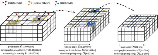
Simplified schematic illustration of nested numerical grids that represent increasingly finer earth structure constrained by shorter-period data from increasingly dense networks on smaller scales. The ideal tomographic model should combine all scales and periods consistently, in the interest of completeness and minimization of artefacts related to scale dependence. A local grid refinement that captures smaller-scale structure enforces a commensurate decrease in the time step needed to propagate the numerical wavefield. Left: For global tomography, where the computational domain has dimensions of |$\mathcal {O}(10.000\, {\rm km})$|, the broad structure is constrained by teleseismic data recorded on the global network. Resolution lengths in global tomography are typically at the order of 100–1000 km (e.g. Panning & Romanowicz 2006; Lebedev & van der Hilst 2008; Nettles & Dziewoński 2008). Centre: Structure on length scales of 10–100 km can be constrained with dense regional networks, using either regional seismicity (e.g. Kissling 1988; Tape et al.2009) or tomography based on noise correlations (e.g. Shapiro et al.2005; Tromp et al.2010). On regional scales, 3-D crustal structure can be resolved when surface waves with sufficiently high frequency are used. Right: Further refinements down to the 1–10 km or even smaller scales can be achieved when dense local networks are available. For numerical wave propagation, the grid spacing is typically a fraction of the propagating wavelength, meaning that the global-scale model (left) has a locally refined grid spacing of |$\mathcal {O}(0.1{\rm -}1\,{\rm km})$|. The resulting time step would be prohibitively small for global wave propagation at any period.
1.4 Objectives and outline
Our principal objective is to develop and apply a full waveform inversion method that incorporates data across a wide range of spatial scales and frequencies. This is intended to yield consistent models of both crust and mantle that will later serve as a basis for inversions to constrain Q and anisotropy.
This paper is organized as follows: in Section 2 we describe the general theoretical background of our method. This includes the decomposition of a multiscale earth model into a family of single-scale models with the help of non-periodic homogenization and the ‘Alternating Iterative Inversion’ (AII) of seismic data at each of the different scales. Section 3 is dedicated to the application of our method to Europe and western Asia, with a focus on the Anatolian region where a particularly dense coverage allows us to constrain the details of both crustal and mantle structure simultaneously and consistently. We verify our model with estimates of crustal depth from receiver functions and the waveform fit to correlations of ambient seismic noise that were not used in the tomographic inversion. In Section 5 we discuss the validity range of our method, as well as alternative strategies.
Since the focus of this paper is on methodological developments and the demonstration of their feasibility, we only provide a brief geological interpretation of the resulting tomographic models. More detailed discussions of geology and the effects of multiscale imaging on models of Q and anisotropy will appear in later publications.
2 THEORY: COMBINING DATA SETS ON MULTIPLE SPATIAL SCALES USING NON-PERIODIC HOMOGENIzATION
2.1 Multi-to-single-scale decomposition
To achieve the incorporation of shorter-period data on smaller scales, we decompose the computational domain and solve multiple forward problems. For this, we define a ‘master model’ that describes earth structure on all accessible scales. Where dense data on smaller scales are available, the grid of the master model is refined accordingly. The central element of our method is the decomposition of the master model into various single-scale models, thereby breaking the bottom-up control of the smallest grid spacing on the global time step. This is illustrated in Fig. 2.
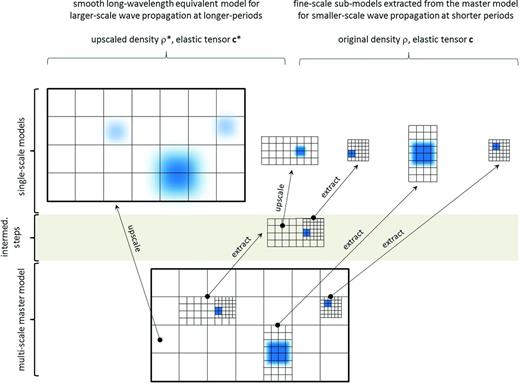
Schematic map view of the decomposition of the multiscale master model (bottom row) into various single-scale models. Shorter-period wave propagation is restricted to the finely gridded subvolumes where dense data on smaller scales are available. Subvolumes can be directly extracted from the master model and incorporated into numerical wave propagation schemes. The construction of larger-scale models from the master model involves the upscaling of the detailed structure m = (ρ, c) to the smooth and long-wavelength equivalent structure m* = (ρ*, c*). For sufficiently long wavelengths, the effective medium is equivalent to the original fine-scale medium. The upscaled model can be implemented on a coarse numerical grid, which reduces computational costs substantially. The decomposition of the master model results in various single-scale models that can be used for numerical wave propagation at appropriate periods without the need for excessive computational resources. In the schematic example shown here, the complete forward problem consists of five independent wavefield simulations in the single-scale models shown in the top row.
First, we confine shorter-period wave propagation on the smaller scales to finely gridded subvolumes, that is to small computational subdomains that contain a tractable number of grid points. Earthquake or noise correlation data from a dense regional array, for instance, can thus be modelled efficiently at short periods without any overhead of grid points outside that particular region.
Secondly, we construct smooth long-wavelength equivalent versions of the small-scale structures in the master model to enable the efficient propagation of longer-period waves. For this we use non-periodic homogenization (Capdeville et al.2010a,b), which upscales the original density ρ and elastic tensor c to smooth long-wavelength equivalents ρ* and c*. The upscaling procedure introduces apparent anisotropy that must be included in the forward modelling. For waves with sufficiently long wavelength, the upscaled model m* = (ρ*, c*) is equivalent to the original model m = (ρ, c), meaning that both produce nearly identical wavefield solutions. Being smooth, the upscaled model can be implemented on a coarse numerical grid, thereby reducing the computational cost substantially. The exemplary global simulation of 30 s waves from Section 1.3 is now independent of the locally refined grid that captures details on a subwavelength scale. A realistic example of the upscaling procedure is provided in Section 3.2.5.
All single-scale models that result from the domain decomposition, contain a tractable number of grid points, either because they comprise a small densely covered region, or because the structure has been upscaled so that it can be represented by a coarse grid. For each of the single-scale models, one independent forward problem is solved. Thus, in the case of the schematic example of Fig. 2, five wavefield simulations must be performed to solve the complete forward problem.
2.2 AII scheme
The multi-to-single-scale decomposition of the master model can be used to construct iterative schemes for the consistent inversion of data sets on various scales. ‘AII’ computes model updates for specific scales sequentially, that is one scale at a time. AII was used for the application presented in Section 3, and it will be described in detail in the following paragraphs. An alternative inversion scheme, ‘Simultaneous Iterative Inversion’, is proposed in Appendix.
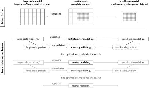
Starting from the initial master model m0, AII computes a smooth long-wavelength equivalent version |$\mathbf {m}^*_0$| using non-periodic homogenization, as illustrated in Fig. 3. The longer-period data on the larger scale are then used to compute an update of the large-scale model, denoted Δm0.1 in Fig. 3. This first step involves (1) the computation of synthetic seismograms for m0.1, (2) the comparison of the synthetic and observed seismograms using a suitable misfit measure (e.g. Crase et al.1990; Fichtner et al.2008; Brossier et al.2010; Bozdağ et al.2011), (3) the computation of sensitivity kernels and a descent direction with the help of adjoint techniques (e.g. Tarantola 1988; Tromp et al.2005; Fichtner et al.2006) and (4) the determination of an optimal step length using a line search (e.g. Nocedal & Wright 1999). The large-scale update Δm0.1 is then added to the initial multiscale master model m0 to produce the updated model m0.1. The values of the large-scale update Δm0.1 at the potentially finer space grid points of the master model are found by interpolation.
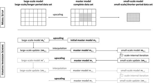
Schematic illustration of Alternating Iterative Inversion (AII). The initial master model m0 is upscaled to a smooth large-scale model |$\mathbf {m}^*_0$| across which the longer-period data are propagated. Using adjoint techniques combined with a gradient-type optimization, an update Δm0.1 is computed. This update is interpolated onto the master model to yield m0.1 from which the small-scale model is extracted for shorter-period wave propagation. Again using adjoint techniques and gradient-type optimization, a small-scale update Δm0.2 is computed. This step can involve more than one iteration with the short-period data. Finally, the small-scale update is added to m0.1 to produce the new master model m1. This procedure is repeated until a satisfactory fit to the data is achieved.
Subsequently, the regionally confined small-scale model is extracted from the master model, and the shorter-period data are modelled. Following the same procedures as before, a small-scale update Δm0.2 is computed and added to the master model to yield the first fully updated master model m1.
Continuing with m1, this sequence of updates is repeated to yield successively improved master models m2, m3, …. The inversion stops when a satisfactory fit to the data is achieved.
There are important variations of this theme. First, the schematic AII presented in Fig. 3 can be extended to include various smaller-scale models by simply marching through a sequence of single-scale models that contribute to a complete update of the master model. Secondly, the computation of an update for a specific single-scale model can involve more than one ‘scale-internal iteration’. In the case of the small-scale model in Fig. 3, for instance, one can iterate many times with the shorter-period data in order to add small-scale updates into a cumulative update Δm0.2. The cumulative update is more likely to be sufficiently significant to have a notable impact on the large-scale structure in the next step of the sequence.
3 APPLICATION: FULL WAVEFORM INVERSION OF EUROPE AND WESTERN ASIA WITH FOCUS ON THE ANATOLIAN REGION
At this stage, we have all ingredients for the simultaneous inversion of seismic data on different spatial scales. To demonstrate the applicability of the method proposed in Section 2, we continue with a full waveform inversion of Europe and western Asia with a particular focus on Anatolia where a dense coverage allows us to constrain the details of crustal structure.
3.1 Data
We consider three-component data on two spatial scales and within two period ranges. A summary of the data is shown in Fig. 4. On the continental (10.000 km) scale we use 14.525 recordings from 84 earthquakes that occurred between 2005 and 2011 mostly along the plate boundaries of Eurasia. We obtained waveform data from the ‘Incorporated Research Institutions for Seismology’ (IRIS), the ‘Observatories and Research Facilities for European Seismology’ (ORFEUS) and the ‘IberArray’ seismic network (Díaz et al.2009). Magnitudes are between Mw = 5.0 and Mw = 6.8, so that finite-source effects can largely be ignored. Periods range from 30 to 200 s, meaning that the data mostly constrain upper-mantle structure.
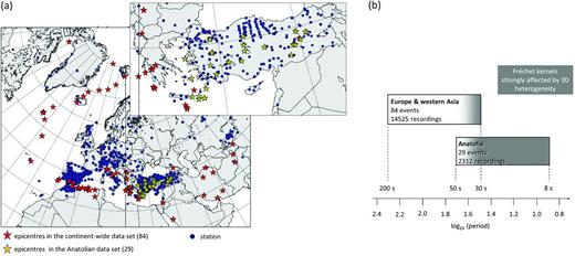
Data summary. Left: Distribution of events in the continent-wide data set (red stars), events in the regional data set (yellow stars) and stations (blue dots). The coverage is particularly dense in Anatolia, where the regional seismicity can be used to put strong constraints on shallow structure above ∼100 km depth, including the crust. Right: Volume and period range of the data subsets for the whole continent (14.525 recordings between 30 and 200 s) and Anatolia (2.312 recordings between 8 and 50 s). The grey-shaded area marks the period range where sensitivity kernels are strongly affected by 3-D heterogeneity.
On the regional (1.000 km) we use data from the Anatolian region recorded on the dense networks of the ‘Kandilli Observatory and Earthquake Research Institute’ (UDIM) and the ‘National Seismic Array of Turkey’ (AFAD-DAD). From the 29 earthquakes considered, we use a total of 2.312 recordings in the 8–50 s period range, which allows us to constrain crustal heterogeneities. Magnitudes in the regional data set range from Mw = 4.7 to Mw = 5.5.
Our data selection was based on the comparison between observed seismograms and synthetic seismograms computed for the 3-D initial model described later in Section 3.2. We only selected seismograms where the noise—estimated from waveforms prior to the P wave—is negligible compared to the differences between observed and synthetic seismograms.
The Anatolian region is effectively covered by data with periods from 8 to 200 s, meaning that both crustal and mantle structure can be resolved. For periods below ∼50 s, sensitivity kernels start to be significantly affected by 3-D structure. This indicates the need for numerical wave propagation and adjoint techniques in this type of tomographic studies (see Figs 4(b) and 5).
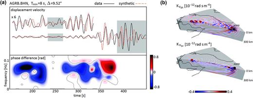
Illustration of the time-frequency phase misfit and corresponding sensitivity kernel for a single source–receiver pair. Synthetic seismograms and kernels are computed for model m41, which is one iteration before our final model m42 that we discuss in Section 3.4. (a) Top: N–S component observed (black solid) and synthetic (red dashed) seismograms for station AGRB in eastern Anatolia and an Mw = 5.1 in southwestern Anatolia (see source–receiver configuration to the right). The first few hundred seconds are amplified for better visibility. Grey shading marks parts of the recordings that were disregarded because the strong dissimilarities between observations and synthetics prevent a meaningful phase measurement. Bottom: Phase difference between observed and synthetic seismograms as a function of time and frequency. Blue corresponds to a delay of an observed waveform relative to a synthetic waveform, and red corresponds to an advance. Delays and advances can occur at the same time for different frequencies. (b) The sensitivity kernels with respect to |$v_{\small SH}$| (top) and |$v_{\small SV}$| (bottom) for the measurement shown to the left. The kernels were computed using adjoint techniques. The position of the source is marked by a red dot. The black dot indicates the receiver position.
3.2 Details of the forward- and inverse-modelling procedure
3.2.1 Forward modelling, misfit quantification and sensitivity kernels
We model our data using a spectral-element discretization of the seismic wave equation, described in Fichtner & Igel (2008). The spectral-element modelling produces accurate solutions of the complete seismic wavefield in strongly heterogeneous media, which is a prerequisite of full waveform inversion that attempts to exploit entire seismograms for the benefit of improved tomographic resolution.
Following the scale- and domain-decomposition concept introduced in Section 2.1, we solve two separate wave propagation problems. On the continental scale, we use elements that are on average 45 km wide. This corresponds to a sampling of ∼2 elements per minimum wavelength for waves with periods above 30 s, which is necessary to obtain accurate numerical solutions. Short-period regional wave propagation is restricted to a 500 km deep volume that contains the Anatolian region, and which is shown in the upper left corner of Fig. 12. Within Anatolia, the average element width is 12 km, to ensure the correct simulation of waves with periods as low as 8 s. The Lagrange polynomial degree for all simulations is 4. Note that, a grid spacing of 12 km anywhere within the continental model would lead to prohibitive computational costs due to the time step reduction required by the CFL stability condition.
To quantify the misfit between observed and synthetic spectral-element seismograms, we use the time-frequency phase misfits introduced by Fichtner et al. (2008) on the basis of suggestions for the comparison of seismograms by Kristekova et al. (2006). For this, we manually select those parts of the seismograms where observed and synthetic waveforms are sufficiently similar to avoid cycle skipping ambiguities. Both observed and synthetic seismograms are then transformed to the time-frequency domain using a Gabor transform. The misfit is then defined as the square of the phase difference between observations and synthetics, integrated over time and frequency and summed over all source–receiver pairs.
The time-frequency phase misfit allows us to incorporate all types of seismic waves, including body and surfaces waves, as well as unidentified waveforms. There is no need to detect isolated phases, meaning that interfering waveforms at short epicentral distances can be measured. Furthermore, the time-frequency phase misfits automatically balance small- and large-amplitude waveforms. For instance, a 5 s time-shift in a large-amplitude surface wave contributes as much to the total misfit as a 5 s time-shift in a small-amplitude P waveform. An example for a time-frequency phase measurement is shown and described in Fig. 5(a).
The presence of potentially strong 3-D heterogeneities, especially within the lithosphere, require the calculation of accurate sensitivity kernels with numerical wave propagation and adjoint techniques (e.g. Tarantola 1988; Tromp et al.2005; Fichtner et al.2006). While the computation of approximate sensitivity kernels via normal-mode summation or ray theory can be justified for mildly heterogeneous models (Lekić & Romanowicz 2011; Zhou et al.2011; Mercerat & Nolet 2012), the strong variations especially in the Anatolian part of the model (see Fig. 12) require fully numerical modelling combined with adjoint techniques. Approximate sensitivity kernels can reduce the convergence speed, thereby preventing the discovery of fine structure that tends to appear during later iterations. The |$v_{\small SH}$| and |$v_{\small SV}$| sensitivity kernels for the measurement in Fig. 5(a) are shown in Fig. 5(b).
3.2.2 Initial model
To accelerate the convergence of the iterative misfit minimization, we implemented a 3-D initial model. The initial crustal structure is a long wavelength equivalent (Fichtner & Igel 2008) of the maximum-likelihood model of Meier et al. (2007a,b) who used a neural network approach to invert surface wave dispersion for crustal thickness and the isotropic S velocity, vS. Within the continental crust, the isotropic P velocity, vP, and density, ρ, are scaled to vS as vP = 1.5399vS + 840 m s−1, and ρ = 0.2277vS + 2016 kg m−3 (Meier et al.2007a). Within the oceanic crust, velocities and density are fixed to the values of the global crustal model Crust2.0 (Bassin et al.2000). As 3-D initial mantle structure we use the isotropic S velocity variations of model S20RTS (Ritsema et al.1999) added to a version of the radially symmetric Preliminary Reference Earth Model (PREM; Dziewoński & Anderson 1981) where the original 220 km discontinuity has been replaced by a linear gradient. The initial P velocity in the mantle is related to the vS variations from S20RTS (Ritsema et al.1999) via a depth-dependent scaling inferred from P, PP, PPP and PKP traveltimes (Ritsema & van Heijst 2002). The initial density structure in the mantle is the one of PREM (Dziewoński & Anderson 1981), and the initial Q distribution is taken from the radially symmetric attenuation model QL6 by Durek & Ekström (1996). Horizontal slices through the initial isotropic S velocity model are shown in Fig. 6.
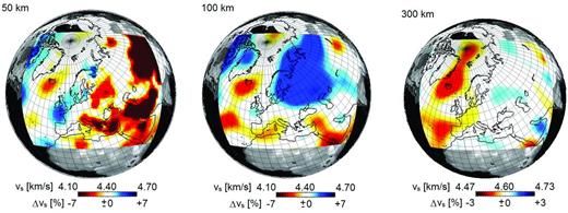
Horizontal slices through the isotropic S velocity, |$v_{{S}}=\frac{1}{3}v_{{\small SV}}+\frac{2}{3}v_{{\small SH}}$|, in the initial model m0 at 50, 100 and 300 km depth. Colour scales are the same as in Fig. 11, which shows the final model m42.
3.2.3 Model parametrization
Within the Anatolian region, we parametrize the earth model by constant-velocity blocks that are 0.15° × 0.15° wide and 5 km deep. Outside Anatolia these blacks are enlarged to 1.0° × 1.0° laterally and 10 km vertically.
3.2.4 Iterative inversion
We minimize the misfit between observed and synthetic seismograms using a variant of the AII introduced in Section 2.2. At the beginning, we only consider the continental-scale data. Following common practice in full waveform inversion (Bunks et al.1995; Virieux & Operto 2009), we start with very long periods from 150 to 200 s in the first few conjugate-gradient iterations and then successively broaden the period range to 30–200 s, to avoid trapping in a local minimum. To prevent the occurrence of artefacts, we slightly smooth the raw gradients. Every ∼3 iterations we update the earthquake source parameters, for which we obtained initial values from the ‘Centroid Moment Tensor’ catalogue (www.globalcmt.org).
After 22 iterations with the continental-scale data, we start to incorporate the shorter-period regional data from Anatolia. Also on this regional scale we successively expand the period range from 35–50 s to 8–50 s, to ensure convergence towards the global optimum. For the next scale-internal cycle we do not revert to a narrower period range, but continue with the period range of the previous cycle. The choice to broaden the period range at a specific point in the iteration is currently a subjective one that is based on the visual inspection of the successively improving waveform fit. The number of scale-internal iterations is 5, meaning that 5 iterations are performed on the Anatolian model before going back to the large-scale model (see Fig. 3).
In total, we perform 20 iterations on the regional Anatolian scale and 22 + 20/5 = 26 iterations on the continental scale, where 20/5 = 4 is the number of updates performed on the continental-scale model during the AII. Thus, the final model formally corresponds to iteration 42. We denote this model by m42 and discuss is principal features in Section 3.4.
3.2.5 Upscaling of small-scale structure in the Anatolian region

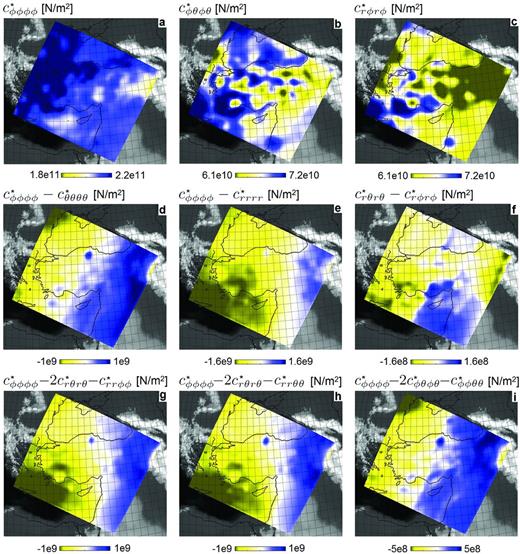
Horizontal slices at 50 km depth through the 3-D distributions of the original elastic parameters and combinations of them. Panels (a)–(c) show the distributions of |$c_{\phi \phi \phi \phi }=A=\rho v_{{\small PH}}^2$|, |$c_{\phi \theta \phi \theta }=N=\rho v_{{\small SH}}^2$| and |$c_{r\phi r\phi }=L=\rho v_{{\small SV}}^2$|, respectively. The combinations of elastic parameters shown in panels (d)–(i) are exactly zero, indicating that the model is radially anisotropic, and that the scaling relations |$v_{\small PH}$| = |$v_{\small PV}$| and η = 1 have been enforced to reduce the dimension of the parameter space.
Horizontal slices at 50 km depth through the 3-D distributions of the smoothed model (ρ*, c*) that is long-wavelength equivalent to the original model (ρ, c) shown in Fig. 7. The horizontal and vertical smoothing lengths are 70 km and 24 km, respectively. This type of smoothing ensures that (ρ, c) and (ρ*, c*) produce nearly identical solutions for periods above ∼30 s. Panels (a)–(c) can be directly identified as smoothed versions of panels (a)–(c) in Fig. 7. The parameter differences shown in panels (d)–(i) are now different from zero but still 1–3 orders of magnitude smaller that |$c^*_{\phi \phi \phi \phi }$|, |$c^*_{\phi \theta \phi \theta }$| and |$c^*_{r\phi r\phi }$|. This indicates that the upscaling introduces a more general form of anisotropy, which remains relatively mild in this specific case.
3.3 Resolution analysis
Before presenting the final model m42 in Section 3.4, we analyse the spatial resolution of the isotropic S velocity structure provided by our combination of data, modelling and misfit quantification. For this we compute 3-D distributions of resolution lengths, which are the position- and direction-dependent half-widths of the tomographic point-spread function. This resolution analysis is based on second-order adjoints and a Gaussian parametrization of the point-spread function, as described in Fichtner & Trampert (2011a,b). Horizontal slices through the resolution length distributions are shown in Fig. 9 for the complete model, and in Fig. 10 with a modified colour scale for the Anatolian subvolume.
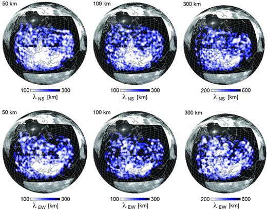
Resolution length for isotropic S velocity structure in N-S direction, |$\lambda _{{\rm\small NS}}$|, (top row) and in E–W direction, λEW, (bottom row) at various depths in the complete tomographic model. The resolution lengths are defined as the half-widths of the tomographic point-spread function in a specific direction. At 50 km depth, resolution lengths are ∼100 km throughout most of central Europe. Due to sparser coverage, resolution lengths are generally larger beneath far-eastern Europe and the Atlantic. Resolution lengths increase with increasing depth because of the diminishing constraints from surface waves that mostly determine shallow structure.

Zoom into the resolution length distribution for isotropic S velocity structure beneath Anatolia, with colour scales shifted towards lower values relative to Fig. 9. Resolution length in N–S direction, λNS, is plotted in the top row, and resolution length in E–W direction, λEW, in the bottom row. The volume where regional short-period data significantly improve resolution is clearly visible in the form of the bright colours throughout Anatolia. Locally, resolution length drops below 30 km.
At 50 km depth, resolution lengths in both N–S and E–W directions are around 100 km or below in most of central Europe, the western Mediterranean and Anatolia. This means that 3-D structures wider than 100 km are resolved, and can thus be interpreted. As a consequence of lower coverage, longer resolution lengths, that is lower spatial resolution, appear beneath the Atlantic, northern Europe and Russia. With increasing depth, resolution lengths increase because of the decreasing influence of surface waves that are mostly responsible for high resolution at shallower depth. At 300 km depth, structures that are less than 200–300 km wide should not be interpreted.
A zoom into the Anatolian region with a colour scale shifted towards lower values, reveals the effect of incorporating shorter-period regional data (Fig. 10). At 20 km depth beneath Anatolia, resolution lengths can locally drop below 30 km, which is close to the wavelength of 8 s shear waves (∼24 km, assuming a propagation velocity of ∼3 km s−1). At 100 km depth, the average resolution lengths are still mostly below 50 km. However, for greater depths, the effect of the regional data diminishes. The additional high-resolution streak extending beneath the Adriatic results from the large number of events in the Aegean region and the dense station coverage in Italy and the Alps (see Fig. 4).
3.4 The tomographic model m42
Figs 11– 13 show slices through model m42. We restrict ourselves to the presentation of the isotropic S velocity vS, computed from |$v_{\small SH}$| and |$v_{\small SV}$| as |$v_{{S}}=\frac{1}{3}v_{{\small SV}}+\frac{2}{3}v_{{\small SH}}$|. Since the focus of this work is on methodological developments, we only provide a brief description of the principal features in model m42, in order to corroborate its plausibility from a geological/tectonic perspective.
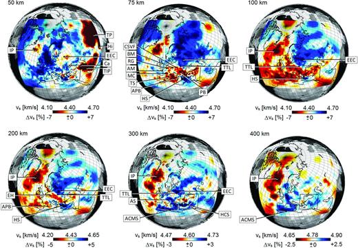
Horizontal slices through the isotropic S velocity, |$v_{{S}}=\frac{1}{3}v_{{\small SV}}+\frac{2}{3}v_{{\small SH}}$|, in model m42. The black quadrilateral around Anatolia marks the volume to which regional shorter-period wave propagation is restricted. Closeups of the detailed structure within the quadrilateral are shown in Figs 12 and 13. Key to marked features: ACMS, Apennine–Calabrian–Maghrebides Slab; AM, Armorican Massif; APB, Alghero-Provençal Basin; AS, Alpine Slab; BM, Bohemian Massif; Ca, Caucasus; CSVF, Central Slovakian Volcanic Field; EEC, East European Craton; HCS, Hellenic–Cyprus Slab; Hi, Himalayas; HS, Hellenic Slab; IP, Iceland Plume; MC, Massif Central; PB, Pannonian Basin; RG, Rhine Graben; TIP, Turkish–Iranian Plateau; TP, Tibetan Plateau; TS, Tyrrhenian Sea; TTL, Tornquist–Teisseyre Line.
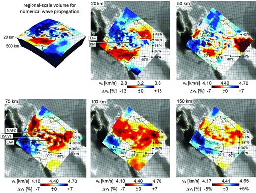
Regional-scale model of Anatolia embedded in the continent-wide model shown in Fig. 11. Displayed is the isotropic S velocity, |$v_{{S}}=\frac{1}{3}v_{{\small SV}}+\frac{2}{3}v_{{\small SH}}$|, in model m42. The upper left corner shows the volume to which we restrict the regional short-period wave propagation. The volume extends from the surface to 500 km depth, and is sliced here at 20 km depth to reveal crustal velocity structure. All remaining panels show the distribution of vS at depths between 20 km and 150 km. Colour scales are the same as in Fig. 11, for the depth levels shown in both figures. Key to marked features: CAV, Central Anatolian Volcanics; KAIVF, Kirka–Afyon–Isparta Volcanic Field; KM, Kirsehir Massif; MM, Menderes Massif; NAFZ, North Anatolian Fault Zone.
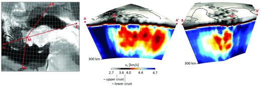
Vertical slices through the Menderes Massif (denoted M) in western Anatolia along the lines indicated in the map to the left. The figures have a vertical exaggeration of 5 to enhance the visibility of crustal structure. The unusual white-grey-black-red-white-blue colour scale is intended to serve the same purpose. The updoming of lower-crustal material (dark grey to black) beneath the Menderes Massif is clearly visible.
3.4.1 Continental-scale structure
Horizontal slices through the continent-wide model from 50 km to 400 km depth are shown in Fig. 11. The inversion also modified the initial crustal model, but crustal structure on the continental scale is unlikely to be well-constrained by data above 30 s period. However, for the Anatolian region, crustal structure is resolved by the regional shorter-period data (see Fig. 10). A discussion of this can be found later in this section.
The 50 km slice in Fig. 11 is marked by the signatures of both crustal and mantle structure. Crustal S velocities well below 4 km s−1 appear beneath the Caucasus, the Turkish–Iranian Plateau, the Himalayas and the Tibetan Plateau where Moho depth can exceed 50 km (Molinari & Morelli 2011). A crustal thickness of ∼50 km also explains comparatively low velocities beneath the East European Craton. S velocities around 4.4 km s−1 and below are found beneath most of the North Atlantic. They most likely result from elevated temperatures beneath the North Atlantic ridge, but also from the periodic injection of high-temperature material from the pulsating Iceland Plume into the North Atlantic asthenosphere (Shaw-Champion et al.2008; Poore et al.2011; Rickers et al.2012). Another notable feature is the elevated S velocities >4.7 km s−1 along western Scandinavia and beneath the Bay of Biscay. Since both regions have comparatively thin crust (<30 km, Molinari & Morelli (2011)), we are in fact likely to see regular mantle velocities that are unaffected by the high-temperature halo of the Mid-Atlantic ridge and the Iceland Plume.
The direct visibility of crustal structure disappears in the 75 km slice of Fig. 11, which is largely dominated by the elevated velocities beneath the East European Craton that locally extend to more than 300 km depth. To the west, the East European Craton is bounded by the Tornquist–Teisseyre Line, which continues as a sharp horizontal transition to more than 300 km. This is in contrast to previous studies that suggest a shallower termination of the Tornquist–Teisseyre Line around 140–200 km depth (Zielhuis & Nolet 1994a,b; Schäfer et al.2011; Legendre et al.2008). The most likely origins of this discrepancy are the accurate numerical modelling and the iterative improvement in our full waveform inversion, but also the exploitation of complete seismograms including all types of seismic waves. The Hellenic slab becomes a pronounced high-velocity feature around 75 km depth, from where it remains clearly visible to below 300 km. The Apennines–Calabrian–Maghrebides and Hellenic–Cyprus slab systems are visible near 300 km depth and below. While, the ‘spatial’ resolution of the slab system is limited by our restriction to continental-scale data with periods above 30 s, the superior ‘amplitude’ resolution of full waveform inversion provides a more realistic picture of the strength of velocity heterogeneities. For instance, from 75 km to around 200 km depth, the Hellenic slab is characterized by vS perturbations of 8–10 per cent. Linearized P-wave tomographies, in contrast, typically find vP perturbations of 1–2 per cent (e.g. Bijwaard et al.1998; Li et al.2008), which extrapolate to vS perturbations of at most 3–6 per cent for a high ΔvS-to-ΔvP ratio of 3. In the North Atlantic region, the Iceland Plume is the most prominent structure, with vS perturbations reaching 10 per cent from 75 km to nearly 200 km depth. Velocity-temperature conversions are based on mineral-physics data (Cammarano et al.2003) or empirical relations (Priestley & McKenzie 2006) yield temperatures above the solidus, suggesting that the low velocities beneath Iceland have a notable contribution from chemical heterogeneities, partial melt or both.
In addition to these broad features, a large number of smaller-scale structures is clearly visible in Fig. 11. These include the elevated velocities of the Armorican Massif and the Alpine Slab, as well as reduced vS beneath the Massif Central, the Rhine Graben, the Bohemian Massif, the Central Slovakian Volcanic Field, the Pannonian Basin, the Eifel Hotspot, as well as the Tyrrhenian Sea and the Alghero–Provençal Basin that are related to extension induced by slab roll-back. Similar structures were found only by Zhu et al. (2012), also using an adjoint- and spectral element-based tomography.
3.4.2 Regional crustal and upper-mantle structure beneath Anatolia
Owing to its elevated seismic risk and importance for Eurasian neotectonics, Anatolia has been the subject of various recent tomographic studies. While crustal structure was imaged with local earthquake tomography (Koulakov et al.2010; Yolsal-Çevikbilen et al.2012), receiver functions (Saunders et al.1998; Vanacore et al.2013) and refraction profiles (Karabulut et al.2003), models of the upper mantle were obtained from teleseismic body and surface waves (Biryol et al.2011; Bakirci et al.2012; Salaün et al.2012). However, a model that constrains 3-D crustal and mantle structure simultaneously and consistently has not been derived so far. The multiscale full waveform inversion developed in Section 2 fills this gap by (1) jointly inverting longer-period (30–200 s) continental-scale data and shorter-period (8–30 s) regional-scale data, (2) accurately simulating seismic wave propagation through complex 3-D media, (3) exploiting all types of seismic waves and (4) correctly accounting for finite-frequency effects.
Horizontal slices through the regional Anatolian model from 20 to 150 km depth are shown in Fig. 12. At crustal depth, around 20 km, lateral velocity variations reach peak values of ±18 per cent. Similarly, strong variations were found by Tape et al. (2009) in a full waveform inversion for the crustal structure of Southern California. The crustal structure is characterized by various high-velocity blocks where vS reaches values around 3.8 km s−1. Beneath central Anatolia, the high velocities mostly correspond to the Kirsehir Massif, which was an independent tectonic block prior to its incorporation into the modern Anatolian plate (Okay & Tüysüz 1999). Near the western margin of Anatolia, elevated vS is mostly the result of crustal extension caused by slab roll-back along the Hellenic trench. The horizontal extension led to the exhumation of lower-crustal material in the Menderes Massif where vS is higher than in the overlying upper crust that was eroded in response to exhumation (e.g. van Hinsbergen et al.2010). A more detailed picture of the updoming lower crust beneath the Menderes Massif is shown in the vertical slices of Fig. 13.
While the 50 km slice in Fig. 12 is dominated by the low velocities within the deep crust of the Turkish–Iranian Plateau, vS at 75 km depth is marked by pronounced low-velocity patches localized directly beneath the Kirka–Afyon–Isparta Volcanic Field and the Central Anatolian Volcanics, thereby suggesting a largely thermal origin. Around 100 km depth, the signatures of the volcanic provinces merge into a broader distribution of lower velocities. They most likely represent shallow upwelling asthenosphere that is believed to result in elevated topography and recent volcanism (Keskin 2003; Sengör et al.2003).
A valuable independent check on the accuracy of the shallow part of m42 is provided by the comparison with receiver function studies. The top panels of Fig. 14 display Moho depth estimates for m42 and from a recent inversion of receiver functions by Vanacore et al. (2013). In m42, we define Moho depth to be where vs reaches 3.8 km s−1, and the receiver function Moho estimates are based on the criterion that vp reaches 6.2 km s−1. Both criteria are to some degree subjective, but the major results are not significantly affected by modifications within reasonable bounds of ±0.1 km s−1. Since our tomography is naturally unable to produce strict vertical discontinuities, we restrict our attention to cases where the vertical vs gradient exceeds 0.05 km s−1 per kilometre, that is where a sufficiently sharp vertical contrast justifies the estimate of a formal discontinuity depth.
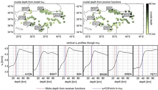
Comparison of crustal structure from model m42 and from the receiver function study of Vanacore et al. (2013). Top: Moho depth distribution estimated from m42 (left) and from receiver functions (right). For m42, we estimate the Moho depth as the depth where vs reaches 3.8 km s−1. In the receiver function study (Vanacore et al.2013), the criterion is vp reaching 6.2 km s−1. Despite the different methodologies and estimates of Moho depth, the results agree to within a few kilometres when strong lateral gradients are absent. Bottom: Collection of vertical vs profiles through m42 for locations where receiver functions are available. Moho depth from receiver functions is plotted as red dashed lines, and Moho depth estimated from m42 as blue dashed line (vs = 3.8 km s−1). A notable difference of ∼20 km between both Moho depth estimates only appears at station FETY, which is located above a strong lateral velocity gradient. (See also the 50 km slice in Fig. 12.)
Despite the different methodologies and data, the Moho depth distributions agree well, which independently confirms that shallow crustal structure in m42 is resolved roughly to the same extent as in receiver function studies. Eastern Anatolia is characterized by comparatively thick crust, whereas the crust in western Anatolia is thin in response to extension caused by slab roll-back. Notable discrepancies between the Moho depth estimates exist where strong lateral velocity contrasts are present. Also, beneath Cyprus, Moho depth estimates do not agree due to complications related to the shallow parts of the Cyprus slab that do not permit unambiguous identifications of the Moho. Compared to the receiver function results, m42 draws a slightly smoother picture of Moho depth variations. This is expected for two reasons. First, the tomography tends to map strong lateral variations in Moho depth into 3-D volumetric velocity heterogeneities. Secondly, receiver functions have comparatively poor control on volumetric velocity perturbations, meaning that strong heterogeneity leads to erroneous Moho depth values. Ideally, both methods should thus be combined.
The bottom panels of Fig. 14 show a collection of vertical profiles through m42 for locations where receiver functions are available. As previously indicated, Moho depth estimates from m42 (blue dashed lines) and from receiver functions (red dashed lines) mostly agree to within a few kilometres, which is small compared to the vertical grid spacing of 5 km in m42. A large discrepancy of ∼20 km can be observed for station FETY in southwestern Anatolia, that is in a region where lateral vs variations of more than 15 per cent (peak-to-peak) over less than 100 km might limit the applicability of the receiver function technique (50 km slice in Fig. 12).
4 MODEL VERIFICATION
To validate model m42, we provide representative examples of fits to data, both used and not used in the inversion.
4.1 Waveform fit
Fig. 15 shows a comparison of observed seismograms (black), synthetic seismograms for the initial model m0 (grey) and synthetic seismograms for the final model m42 (red) for two shallow events in western (A) and eastern (B) Anatolia. Data from both events were used to constrain m42. The shortest period is 8 s. At most stations, synthetic surface waveforms computed for the initial model arrive too late, indicating that the initial crustal velocities are consistently too low. Indeed, above ∼100 km depth, lower than average velocities are distributed throughout the Anatolian region in the initial model (Fig. 6), instead of being localized along the North Anatolian Fault and around few volcanic provinces, as in the final model (Figs 12 and 13). Body and surface waves in synthetic seismograms computed for the final model agree well with the observations in both phase and amplitude, despite the fact that the time-frequency phase misfits are unaffected by an amplitude scaling of the data. Remaining differences between observations and synthetics most likely result from the presence of noise and the unavoidably incomplete physics in the wave propagation simulations.
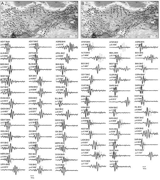
Representative comparison of observed seismograms (black), synthetic seismograms for the initial model m0 (grey) and synthetic seismograms for the final model m42 (red) for two events in western (A) and eastern (B) Anatolia. The source locations are marked by a blue star. The shortest period is 8 s. While the synthetic waveforms for the initial model mostly arrive too late, the synthetics for the final model generally agree well with the data.
4.2 Fit to noise-correlation data not used in the inversion
Since the fit to data used in the inversion is expected, we furthermore assess the quality of m42 with independent data not used to constrain the final model. For this we compute correlations of vertical-component ambient seismic noise between two reference stations (BALB and HOMI) and collection of other stations throughout Anatolia. In the idealistic case where seismic noise is generated by sources covering a closed surface around each receiver pair, the correlation function approximates the interstation Green’s function (e.g. Lobkis & Weaver 2001; Wapenaar 2004; Shapiro et al.2005). It follows that the match between noise correlations and numerical interstation Green’s functions can serve as an independent and semi-quantitative proxy for the quality of an earth model.
The comparison between a collection of interstation correlations of vertical-component seismic noise and the corresponding numerical Green’s functions is shown in Fig. 16. Since the amplitudes of noise correlations depend strongly on the noise source distribution (Tsai 2009; Cupillard & Capdeville 2010), we scale the maximum amplitudes to 1 and restrict ourselves to the analysis of the phase match. The reference stations BALB and HOMI are located in western and eastern Anatolia, respectively, thereby providing a good azimuthal and directional coverage of the region. Whenever clear waveforms emerge from the noise correlations, the phases agree to within a fraction of the dominant period which is 10 s.
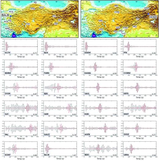
Comparison between the causal part of observed ambient seismic noise correlations (black) and numerical Green’s functions computed for model m42 (red). The reference stations are BALB in western Anatolia (left) and HOMI in eastern Anatolia (right). Traces are normalized to a maximum amplitude of 1. Whenever a clear surface waveform emerges from the noise correlation, the phase matches the numerical Green’s function to within a fraction of a period. This remarkable match is an independent indication that the imaged 3-D structure is realistic and required. It, furthermore, highlights the predictive capability of the model that may be used to improve seismic source inversions.
This result indicates that the waveform data in the inversion have not been overfit, and that model m42 is reliable and well constrained. It, furthermore, suggests that noise sources in the Anatolian region are sufficiently well distributed to provide good approximations at least for fundamental-mode surface wave Green’s functions when noise from station pairs is correlated. A quantitative comparison of higher-mode surface and body waves is currently not possible, as it requires a perfectly homogeneous distribution of both mono- and dipolar noise sources that does not exist on Earth (Halliday & Curtis 2008; Kimman & Trampert 2010).
The ability of m42 to reproduce a data type not used in the inversion is particularly encouraging. This opens new perspectives not only in noise tomography but also in seismic source studies that rely on detailed and well-constrained 3-D earth models.
5 DISCUSSION
5.1 Potentials and limitations
In Section 3 we presented the simplest version of the more general inversion scheme introduced in Section 2: A ∼1000 km scale regional data set embedded within a ∼10.000 km scale continental data set. This application can and will be extended by incorporating additional data from dense arrays that record earthquakes at short epicentral distance. Where seismic activity is too weak, noise correlations can be used instead (e.g. Shapiro et al.2005; Tromp et al.2010). The extension of the previously presented multiscale full waveform inversion has the potential to increase significantly our knowledge of small-scale structure and scale-dependent properties.
Nevertheless, limitations remain. They include the poor station coverage in some of the less accessible regions of the Earth, but also attenuation that conceals valuable information about 3-D structure. It follows, for instance, that intrinsic anisotropy beneath the poorly covered oceans may remain less well constrained than intrinsic anisotropy beneath the continents where small-scale heterogeneities can be imaged with increasing reliability.
5.2 Alternative approaches
Our multiscale full waveform inversion relies on the computation of smooth, long-wavelength equivalent models using zeroth-order, non-periodic homogenization. In the example shown in Section 3, the forward-modelling errors introduced by the replacement of the original model by its smoothed version are negligible compared to the differences between observed and synthetic seismograms. This is because the smoothing length is not orders of magnitude larger than the correlation length of heterogeneities in the original model. In the presence of stronger heterogeneities, higher-order homogenization may become necessary.
An alternative approach could be the use of local time substepping methods that have been developed for a variety of numerical schemes (Tessmer 2000; Kang & Baag 2004; Dumbser et al.2007; Madec et al.2009). The time step is reduced locally within a model subvolume where the mesh is refined to sample small-scale structure. Matching conditions are enforced at the boundaries between subvolumes with different time steps. While being subjectively more elegant than the externally computed homogenized earth model, local time substepping is still computationally more expensive because additional time steps must be computed within the refined portions of the mesh, and because the total number of grid points is significantly larger.
5.3 Combination with other tomographic techniques
The fundamental problem that motivates this work, is the limitation of computational resources that complicate the simulation of high-frequency wave propagation. The multiscale full waveform inversion developed in Section 2, overcomes this problem when high-frequency wave propagation is restricted to sufficiently moderate epicentral distances. However, the fully numerical simulation and inversion of teleseismic waves at frequencies around 1 Hz will remain impossible for many years to come. This limits the resolution of 3-D earth structure that is typically constrained by the arrival times of high-frequency body waves, for example, deeply subducted slabs or the deep structure of mantle plumes. Therefore, future research needs to accomplish the combination of various methods in order to make the complete seismic spectrum accessible for tomography. These methods include ray-based finite-frequency traveltime tomography (Dahlen et al.2000; Tian et al.2009), the inversion of the Earth’s eigenfrequencies using normal modes (e.g. Giardini et al.1987) and full waveform inversion that exploits the intermediate frequency range in an optimal way.
5.4 Implementation of and inversion for crustal structure
A key element in the tomographic inversion for 3-D crustal structure is the parametrization of crustal discontinuities in the initial model. Intuitively, one may argue that initial crustal structure, including discontinuities, should be implemented as accurately as possible using the best available crustal models. This approach was adopted, for instance, by Tape et al. (2010) and Zhu et al. (2012). However, discontinuities will remain at their initial depths during the inversion because any model update is smooth. Consequently, shallow structure will be biased by the unavoidable inaccuracies of initial crustal models.
As an alternative, we decided to implement an initial model where crustal discontinuities are smoothed, thereby following the approaches of Fichtner & Igel (2008) and Lekić et al. (2010). Crustal discontinuities, and the Moho in particular, are represented by vertical gradients. The depth and the sharpness of the gradients can change easily during the inversion. Biases from incorrect initial Moho depths can therefore be avoided. However, the method will never retrieve an exact discontinuity—in case it is present in the real Earth.
Ideally, one should combine full waveform inversion with proper finite-frequency receiver functions to invert explicitly for volumetric and interface properties. More research in this direction is still needed.
6 CONCLUSIONS AND OUTLOOK
We developed and applied a multiscale full seismic waveform inversion that is capable of simultaneously resolving the details of crustal and mantle structure by integrating seismic data across a wide range of spatial and temporal scales. Our method is based on the decomposition of a multiscale earth model into various single-scale models using 3-D non-periodic homogenization. Each of the single-scale models can be represented by a sufficiently small number of grid points that enables efficient numerical wave propagation. An AII scheme built on spectral-element simulations and adjoint techniques can then be used to consistently combine data on various scales into one earth model.
We demonstrated the applicability of our method in a full waveform inversion for Europe and western Asia with a focus on Anatolia where dense regional data are available. While the complete continent is covered by data with periods from 30–200 s, structure beneath Anatolia is additionally constrained by 8–50 s waveforms. This broadband coverage is able to resolve crustal and mantle structure simultaneously. Resolution lengths drop below 30 km within the Anatolian crust, and are mostly below 50 km within the underlying mantle to 200 km depth. The final model, m42, reveals subtle structural features of the European upper mantle, including, for instance, the Bohemian Massif, the Rhine Graben and the system of lithospheric slabs in the western Mediterranean. The Anatolian submodel shows clear signatures of local volcanic provinces, the North Anatolian Fault Zone (Fichtner et al.2013) and lower-crustal upwellings in the extensional regime of western Anatolia.
In addition to a quantitative resolution analyses we performed various tests to assess the quality of our model: We find that crustal depths estimated from receiver functions agree to within a few kilometres with estimates of crustal depths from model m42. Synthetic seismograms for m42 match observed seismograms in great detail, including both body and surface wave parts on all three components. Furthermore, our model explains correlations of ambient seismic noise that have not been used in the inversion.
The purpose of this paper is to demonstrate the multiscale methodology and its applicability to real data, with Anatolia serving as the ideal testbed. The incorporation of data from other regions, including Iberia and the North Atlantic (Rickers et al.2013), is work in progress. At this stage, our method has the potential to considerably further our understanding of crust–mantle interactions that shape the nature of plate tectonics. In future studies, it will be used to improve images of strongly scale-dependent properties in the mantle that rely on accurate 3-D models of the crust.
AF was funded by The Netherlands Research Center for Integrated Solid Earth Sciences under project number ISES-MD.5. TT thanks the Alexander von Humboldt-Stiftung, ÜBİTAK, TÜBA and İTÜ for partial financial support. ES was supported through Australian Research Council Grants. The contribution of YC was supported by the ANR mémé (ANR-10-Blanc-613) project. We would like to thank AFAD-DAD and BU-Kandilli Observatory-UDIM for providing earthquake data set on Turkish stations. This work would not have been possible without the support of Yesim Çubuk and Seda Yolsal-Çevikbilen. Elizabeth Vanacore kindly provided the results of her receiver function study, shown in Fig. 14. We are grateful to Theo van Zessen for maintaining the HPC clusters STIG and GRIT in the Department of Earth Sciences at Utrecht University. Numerous computations were done on the Huygens IBM p6 supercomputer at SARA Amsterdam. Use of Huygens was sponsored by the National Computing Facilities Foundation (N.C.F.) under the project SH-161-09 with financial support from the Netherlands Organisation for Scientific Research (N.W.O.). AF also would like to acknowledge the hospitality of Brian L. N. Kennett, Hrvoje Tkalčić, Malcolm Sambridge and Giampiero Iaffaldano from The Australian National University, where most of this manuscript was written. The very constructive and insightful criticism of the reviewers Jeroen Ritsema and Stéphane Operto helped us to improve the manuscript substantially. Finally, AF would like to thank his most careful and patient reader, Moritz Bernauer, for asking just the right questions and for finding all those errors that the author never manages to find himself.
REFERENCES
APPENDIX: SIMULTANEOUS ITERATIVE INVERSION
As an alternative to the Alternating Iterative Inversion (AII), introduced in Section 2.2, we propose an inversion scheme based on the determination of a joint step length for updates on the various scales. This ‘Simultaneous Iterative Inversion’ (SII), illustrated in Fig. A1, starts with the construction of an upscaled version of the initial model m0, denoted |$\mathbf {m}^*_0$|, and with the extraction of the regionally confined small-scale initial model. Using numerical wave propagation combined with adjoint techniques, two gradients are computed: (1) a large-scale gradient from the longer-period data, and (2) a small-scale gradient from the shorter-period data. Both gradients are added to form a master gradient, g0, which determines a descent direction. Adding both gradients corresponds to adding the misfit functionals on the different scales. A line search can then be used to determine the optimal step length. This line search involves the upscaling of test models for specific step lengths. When the optimal step length is found, the initial mast model m0 can be updated to master model m1. The procedure is then repeated until a satisfactory fit to the data is achieved.
Schematic illustration of the ‘Simultaneous Iterative Inversion’ (SII). The initial master model m0 is upscaled to its smooth large-scale version |$\mathbf {m}_0^*$|, and the regionally confined small-scale model is extracted. Using adjoint techniques, gradients for both models with their respective data sets are computed, and the gradients are combined into a master gradient g0. A line search determines the test model with the lowest misfit. The line search itself requires upscaling from the master test models to smooth large-scale test models. The optimal master test model is set equal to the new master model m1. This procedure is repeated until a satisfactory fit to the data is achieved.
The computational costs for one iteration in SII are similar to those in AII, but the relative performance of both schemes in terms of convergence speed and ease of implementation, remains to be tested.
