


Summary
High-rate (5Hz) GPS records observed in the near field following the magnitude 7.2 El Mayor—Cucapah earthquake that occurred in northern Mexico on 2010 April 4 are compared with broad-band seismograms. The high-rate GPS displacement records are consistent with the twice-integrated strong-motion seismic records in the near field where broad-band seismograms are clipped due to strong shaking. Agreement degrades at distances greater than about 150 km from the epicentre where displacement amplitudes approach the noise level of GPS seismograms. Using high-rate GPS data the focal mechanism of the main shock is estimated and is shown to be consistent with teleseismic estimates. The result is seen as confirmation that high-rate GPS observed at near-field stations can be applied together with teleseismic seismometers to yield better information about earthquake rupture properties and parameters.
1 Introduction
The Global Positioning System (GPS) is a constellation of satellites used primarily for navigation purposes to determine position with a precision of about 1 m in real time. A much higher horizontal precision approaching ∼1 mm is achievable via data processing in non-real-time, a fact that has been well exploited to determine long-term deformation in the shallow crust by analysing changes in position on a daily basis (e.g. Segall & Davis 1997; Larson et al. 1997, 2004; Wang et al. 2001; and many others). Until recently, the use of GPS instruments for seismological purposes has been the subject of appreciably less work. Interest in this application has been growing, however, because near large earthquakes broad-band seismometers tend to clip and, although strong-motion accelerometers do not, the conversion of acceleration to displacement is degraded by large drifts caused by tilts and the non-linear behaviour of the accelerometer (e.g. Trifunac & Todorovska 2001). For GPS to be used for seismology, much higher sample rates approaching or exceeding 1 sample-per-second are required.
The seismological potential of GPS was first investigated by Hirahara et al. (1994), Ge (1999), Ge et al. (2000) and Bock et al. (2000) who showed that GPS could measure large displacements or instantaneous geodetic positions over very short time spans. Larson et al. (2003) first observed dynamic seismic displacements using GPS following the 2002 magnitude 7.9 Denali Fault (AK) earthquake and demonstrated the similarity between the displacement seismograms determined from GPS and broad-broad seismometers. Bilich et al. (2008) further advanced these investigations. These were largely far-field observations (many hundreds of kilometres) made possible by the strong directivity of the earthquake along the azimuth to distant GPS and seismic instruments. The principal interest in the application of GPS seismology is as a strong motion instrument in the near field (Larson 2009). The feasibility of near-field GPS seismology was demonstrated following the 2003 magnitude 6.5 San Simeon (CA) earthquake (Hardebeck et al. 2004; Wang et al. 2007), the 2003 magnitude 8.0 Takachi-Oki earthquake in Japan (Emore et al. 2007), and the 2009 magnitude 6.3 L’Aquila earthquake in Italy (Avallone et al. 2011). GPS seismology has also been shown to be useful in fault rupture inversions alone or in concert with strong-motion and teleseismic data (Ji et al. 2004; Miyazaki et al. 2004; Langbein et al. 2005; Kobayashi et al. 2006; Yokota et al. 2009) and for measuring surface wave dispersion (Davis & Smalley 2009). Blewitt et al. (2006) demonstrated the effectiveness of GPS to estimate earthquake magnitudes rapidly for tsunami warning and Gomberg et al. (2004) used GPS seismology to study earthquake triggering.
The 2010 April 4 magnitude 7.2 earthquake (22:40:41.77 GMT), referred to as the El Mayor—Cucapah earthquake, struck Baja California approximately 65 km south of the US–Mexico border (Fig. 1a). This earthquake ruptured along the principal plate boundary between the North American and Pacific plates with a shallow focal depth. Surface rupture of this earthquake extended for about 120 km from the northern tip of the Gulf of California northwestward nearly to the international border, with breakage on several faults.
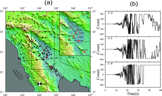
(a) Location of the El Mayor—Cucapah earthquake and the distribution of selected GPS stations. Triangles represent the GPS stations: hollow triangles are the stations >w200 km from the epicentre while the solid triangles are the stations closer than 200 km. The ’beachball’ is the Harvard-CMT focal mechanism of the main shock located at the epicentre. Grey circles are aftershocks with magnitudes larger than M4.0. The red stars are locations of the high-rate GPS stations used in the inversion for the focal mechanism, and the largest red star is the epicentre of the main shock. The red square and red diamond are the locations of the broad-band seismic station and the strong motion seismic station of Fig. 5. The white contour lines show strong motion of the earthquake, with units in percent of gravitational acceleration, g. The inset enlarges the area outlined by the black rectangle. (b) Clipped broad-band seismograms following the El Mayor—Cucapah earthquake recorded at the broad-band seismograph at station SWS, located about 100 km from the epicentre.
The earthquake occurred where the southern California shear zone, a system of continental parallel right-lateral faults including the San Andreas, San Jacinto and Elsinore faults, connects with a system of transform faults and active spreading centres in the Gulf of California. A high level of historical seismicity has been observed in this region, and this fault system has been active in recent years although the previous large earthquake occurred in 1892 (USGS). The Pacific Plate is believed to move northwestward with respect to the North American Plate at a speed of about 50 mm yr–1. The principal plate boundary in northern Baja California consists of a series of northwest-trending strike-slip faults that are separated by pull-apart basins. The Harvard focal mechanism solution shows that the El Mayor—Cucapah earthquake is a NW–SE dextral lateral strike-slip event, which is consistent with the strike-slip movement of the southeastern part of the Laguna-Salada fault system. However, this earthquake is a rather complex event. Hauksson et al. (2011) found that the main shock possibly started with a ∼M6 normal faulting event, followed ∼15 s by the main event, which included simultaneous normal and righ-lateral strike-slip faulting. Based on the finite fault inversion, Wei et al. (2011) demonstrated that the main shock may have begun with east-down motion along faults on the eastern edge of the Sierra El Mayor, then ruptured bi-laterally along the Sierra Cucapah fault and the newly detected Indiviso fault, including both transform lateral slip and ridge extension simultaneously. Both the global moment tensor solution (GCMT, http://www.gcmt.org and Hauksson et al.'s work show that the main shock may contain a significant non-double-couple component, caused by the complexity of the subsurface fault geometry and the source process, specifically the antidipping fault planes.
The main shock lasted over 40 s (Wei et al. 2011) and caused strong shaking in the near field. Based on the USGS analysis, the peak ground acceleration (PGA) recorded by strong motion seismometers was as large as 0.59 g. Even at epicentral distances greater than 100 km, the PGA was still over 0.1 g for some stations (Fig. 1a). For this reason, most of the broad-band seismometers close to the epicentre clipped. An example is shown in Fig. 1(b), which is recorded by a broad-band seismic station SWS at an epicentral distance of about 100 km.
Because the surface waves of these broad-band seismograms are clipped, it is difficult to obtain detailed estimates of the source rupture process using seismic records alone. Thus, other kinds of instruments that are not as seriously affected by strong ground motions are needed to detect the surface displacement. At present, strong motion seismometers and high-rate GPS receivers are the two major candidate instruments. However, because strong motion seismometers can only detect the acceleration of the ground motion, double integration is needed to obtain the displacement, which potentially results in bias such as baseline floating. Although methods have been developed to deal with this problem (e.g. Boore 2001), the accuracy of the integrated ground motion displacement is well below direct measurement. On the other hand, the GPS receivers directly record displacement. Another difference comes from the dominant frequency band between these two kinds of instruments. Strong motion seismometers are designed to detect the large ground accelerations, which makes them mainly focus on high frequency signals. In general, the dominant frequency band of strong motion seismometers range between 0.08 and 100 Hz. However, GPS receivers are designed to provide location information of the site, which makes them more suitable to detect longer period signals. For 5 Hz high rate GPS receivers, the dominant frequency band ranges theoretically from 0 (static displacement) to 1 Hz, but actually 1–1000 s because of various effects (Larson et al. 2007). Strong motion and high rate GPS records, therefore, are complementary for recording near-field signals. Furthermore, to minimize the effects of uncertainties in the structural model, lower frequency signals are more useful for determining the source parameters. Thus, the high rate GPS data are better suited to study source focal mechanisms. In this work we use high-rate GPS records to obtain near field-ground motions of the El Mayor—Cucapah earthquake and then apply these data to estimate the source mechanism of the main shock to test the applicability of high rate GPS data to the inversion of earthquake focal mechanisms.
2 High-Rate Gps Data and Processing
2.1 Data
The Plate Boundary Observatory (PBO) of EarthScope is a geodetic observatory designed to characterize the three-dimensional strain field across the active boundary zone between the Pacific Plate and the western United States. To obtain the long period deformation field as well as short-term dynamic motions, two sample rates are used: one sample per second (1 Hz) and five samples per second (5 Hz). The sampling rate of high-rate GPS receiver is 5 Hz. Such high-rate GPS data can be used to analyse earthquakes at frequencies up to 2.5 Hz. Because the El Mayor—Cucapah Earthquake occurred after construction of the PBO, it was well recorded not only by seismic stations but also by low-rate and high-rate GPS receivers with a 5 Hz sampling rate in the United States.
To estimate the displacement waveforms, we compute the location of the GPS station through the network based, single-epoch resolution of integer-cycle phase ambiguities, which is similar to the method used by Bock et al. (2000, 2011). Because the original GPS data may be contaminated by bias, if the 1 Hz record contains bias in 1 s, then the displacement data will carry bias in this second. On the other hand, although the 5 Hz record may also contain bias, there are five epochs in 1 s, which allows for a more stable result for the 1-s segment. Thus, the resolved location from the higher sampling rate data is usually more stable and more reliable than that from the lower sampling rate data. For this reason, we use 5 Hz data instead of the 1 Hz GPS data. In this work, we acquired high-rate GPS data from GPS stations within 250 km of the epicentre (Fig. 1a). Seven stations are located in the region where PGA is higher than 0.22 g and around 20 stations are situated where PGA is larger than 0.1 g. This distribution provides the opportunity to observe strong ground motion and co-seismic surface displacement of the main shock. We use the high-rate GPS algorithm to solve for the displacements, then correct the displacement record, and finally use the corrected displacements to study the mechanism of the main shock.
2.2 Data Processing
There are several differences between the methods for processing the high-rate GPS data and traditional (30 s sampling) GPS data. The most significant difference is related to the technique of eliminating the GPS satellite clock errors and multipath errors. We process the high-rate GPS data similar to the routine method applied in the GAMIT software developed at MIT (Herring et al. 2010), which includes the following steps. First, high-rate GPS satellite clock corrections are estimated by using high-rate GPS data obtained from globally distributed receivers with precise satellite orbits and low-rate clocks. In contrast to the satellite clock, the satellite orbit can be safely interpolated onto the satellite's position at any time using a high-degree polynomial (Schenewerk 2003). Second, we use the track module of GAMIT to estimate high-rate receiver coordinates based on high-rate GPS data, the precise satellite orbits, and high-rate satellite clocks from the first step. The reference site should be distant from the main shock and is chosen to be station P553, which is about 440 km from the epicentre. In this study, carrier-phase ambiguities are estimated as floating point values, the ionosphere-free linear combination is used to eliminate ionospheric effects (Herring et al. 2010), and the tropospheric delays are modelled using a random-walk stochastic process (Blewitt 1990). In the last step, because the high-rate GPS data contains some noise (mainly multipath effects), to obtain more accurate solutions, especially for surface displacements caused by earthquakes, the final GPS data require further filtering. Sideral filtering was suggested by Genrich & Bock (1992) and was modified by Choi et al. (2004) by considering the satellite repeat time offset to a sidereal day. Here we use the modified sideral filtering method to reduce the multipath effects. Further, a wavelet transform method (Daubechies 1988; Hu et al. 2006) is also used to de-noise the high-rate GPS results.
2.3 Gps Data Correction
Although high-rate GPS records are free from clipping, further corrections are needed to obtain reliable ground displacements. Among these corrections the most important are the removal of linear trends and setting displacement before the arrival of seismic signals to zero (Fig. 2). Fig. 2(a) shows a high-rate GPS seismogram with a long period trend. Fig. 2(b) shows an abrupt jump around 70 s in the record, which is not caused by the earthquake because it occurs before the first arriving seismic phase.
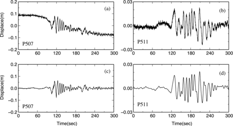
Correction of high-rate GPS data. (a) North–South component GPS record showing a linear trend (GPS site P507, approximately 109 km from the epicentre). (b) North–South component GPS record illustrating signals arriving before the seismic waves (GPS site P511, approximately 181 km from the epicentre). (c) GPS record corrected by removing a linear trend (GPS site P507). (d) GPS record corrected by removing the background signals (GPS site P511). All records are bandpass-filtered from 3.3 to 100 s period.
In this study, we use the following methods to remove these disturbances. (1) For the linear trend, the records before the first arriving seismic phase define the pre-arrival background displacement and the signals long after the earthquake signals have passed are taken as the post-arrival background displacement. We then fit linear trends to the pre- and post-arrival background displacement records separately. If the two trends are close to each other, we remove the average fitted trend from the whole seismogram. If the trends are not similar, we remove the pre-arrival and post-arrival trends separately. For the earthquake signal, we extend the trend of the post-arrival part of the record backward in time and then find the trend in the earthquake signal and remove it. (2) For the long period variations of the background displacement, we first find the dominant period band of the variation and then we build a wavelet bandpass filter bank to remove noise by using an orthogonal wavelet transform based on the 32-order Daubechies wavelet (Daubechies 1988). The wavelet bandpass filters have advantages over the usual FIR digital filter in processing seismic signals by filtering the signal into narrow frequency bands with good frequency response but causing no phase shift and exhibiting no Gibbs phenomenon (Hu et al. 2006). 5 Hz GPS records include all signals within the Nyquist frequency band of 0–2.5 Hz. We use an eight-level wavelet filter bank to filter the records into a new data set in the subband of 2.5/24–2.5/28 Hz; that is, in the period band of 6.4–102.4 s. Figs 2(a)–(d) show the raw and filtered GPS records of P507 and P511, respectively. The comparison indicates that most disturbances in the 5 Hz GPS records are removed. We use the corrected GPS records as seismic data to study earthquakes.
Compared with broad-band seismograms, GPS data are free from clipping, which makes them important for obtaining the near-field displacement. However, resolving the displacement from GPS records requires taking information about the ionosphere, troposphere and the orbit into account, which will be unavoidably contaminated by these disturbances. On the other hand, broad-band seismometers are only sensitive to the motion of the ground and are free from atmospheric disturbances, and the pressure of the atmosphere only weakly affects seismometers. Thus, broad-band seismograms are much more accurate and sensitive to the seismic signals and are more suitable in monitoring the far field seismic signals than high-rate GPS receivers.
3 Comparison Between Seismograms and High-Rate Gps Records
Using the methods described earlier, time-series of horizontal and vertical displacements for 26 high-rate (5-Hz) GPS stations from PBO are obtained. The average error of displacement on the east–west and north–south components is 4.2 and 5.4 mm, respectively. However, the error on the vertical component is about 13 mm, more than twice as large as the horizontal components, because atmospheric disturbances cannot be eliminated as effectively. We analyse the characteristics of the high-rate GPS data here and compare them with seismograms recorded by far-field (<150 km) broad-band seismic stations and near-field (<150 km) strong motion seismometers.
Horizontal displacements of representative GPS stations are plotted in Fig. 3, where the records are aligned by the origin time of the main event (from SCSN). Hand-picked first arrivals indicate an apparent move-out speed of about 3.4 km s–1, which is much slower than the P-wave speed. Because this earthquake initiated weakly (Wei et al. 2011), the P-wave signals apparently are blurred by noise in the high-rate GPS records. The first arrivals, therefore, are S waves in the GPS records. Researchers should be aware that this muting of the P-wave arrivals may affect finite fault inversions.
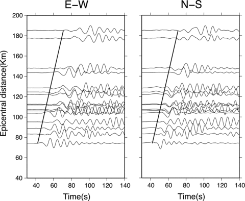
East–West and North–South components of the ground displacements observed with the 5 Hz GPS data. The stations are ordered by epicentral distance. The thick black lines show a move-out with speed of ∼3.4 km s–1.
The dynamic response of the receiver is important to evaluate data quality. To check the ability of high-rate GPS records to detect seismic signals, horizontal records from the station P496, which is 62 km from the epicentre, are chosen to analyse the dynamic responses (Fig. 4a). Peak surface displacements at this station are up to 53 and 57 cm on the E–W and N–S components, respectively, which are much higher than the noise level. Fig. 4(b) shows the spectrum of the three components at frequencies below 1 Hz. Signal power mainly concentrates between 0.01 and 0.3 Hz, and decreases rapidly from 0.25 to 0.5 Hz. This dominant frequency band (0.01∼0.3Hz) is appropriate to analyse medium to strong earthquakes. Signal power at frequencies higher than 1 Hz is quite weak and contributes only negligibly to the integrated signal.
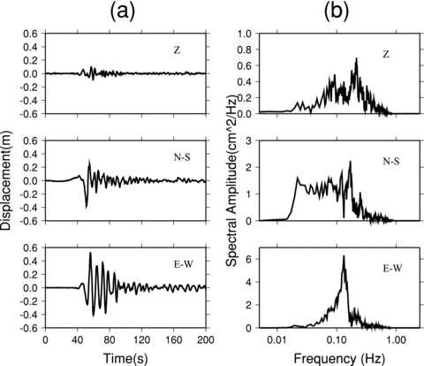
Displacements and spectral amplitudes of GPS records at site P496, approximately 62 km from the epicentre. (a) Displacements on E–W, N–S and vertical components. (b) Spectral amplitude distribution of the high-rate GPS records.
To quantitatively evaluate the quality of high-rate GPS records, we compare them with records from seismometers. An example is shown in Fig. 5(a) in which the record from GPS station P496 is compared with the displacement integrated from a strong motion accelerograph record (NO. 5058). The two stations are located 61–62 km from the epicentre and are separated by less than 1 km, so their displacement seismograms should be similar. We find that the two measurements of displacement are largely consistent, especially in the frequency band from 0.08 to 0.3 Hz. Thus, high-rate GPS measurements can be used to monitor the near-field displacement similarly to strong motion seismometers. On the other hand, the integration of the accelerometer twice to get the displacement tends to amplify biases and distort the true signal. It is, therefore, generally more difficult to correct strong-motion records than GPS records. For these reasons, high-rate GPS records can also be used as a calibration for correcting strong-motion records.
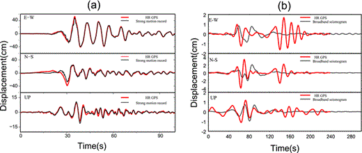
Comparisons of the seismic waves observed on seismometers with the high-rate GPS records. (a) Comparison of 5 HZ GPS displacement record at station P496 (62 km from the epicentre) and the displacement record obtained by twice integrating data from the strong motion accelerograph station 5058 (61 km from the epicentre). The distance between GPS station P496 and strong motion station 5058 is less than 1 km, the GPS signal has been bandpass filtered from 50 to 0.2 s period. (b) Comparison of the 5HZ GPS displacement record at station P472 and the displacement records at broad-band station 109C, which belongs to USArray and was obtained by integrating velocity to displacement. The distance between the receiver and the epicentre of the El Mayor—Cucapah earthquake is 204 km, and the distance between GPS station P472 and seismic station 109C is negligible. The reference zero time is the time of the main shock.
Because of the abundant high-rate GPS and strong motion records of the El Mayor –Cucapah earthquake, several studies have compared the high-rate GPS data and the strong motion accelerograms (e.g. Bock et al. 2011; Allen & Ziv 2011). Our results confirm these earlier studies. Small differences derive from the static displacement, which may due to the filtering effect and the wavelet transform.
High-rate GPS data not only detect strong near-field signals, but also record seismic waves in the far-field, as Larson et al. (2003) demonstrated for the Denali Fault earthquake. Thus, we also compare far-field high-rate GPS data with broad-band seismograms. An example is shown in Fig. 5(b). The record from GPS station P472 is compared with the displacement from broad-band station 109C. The distance between the two stations is under 100 m and epicentral distance is ∼204 km. Here, all seismograms are filtered from 10 to 50 s period. The early arriving body waves are in reasonable agreement with the seismograms, but the GPS records are enriched in higher frequencies. However, in the GPS record there is an unexpected signal following the seismic signal between 120 to 200 s after the main shock, as shown in Fig. 5(b). This signal is also observed at other GPS sites. This later arrival is an artefact caused by data processing. We use one site as a reference site and the displacement shown in Fig. 5(b) is just the displacement of the target site relative to that at the reference site. Although the reference site is farther away from the epicentre than the GPS site, it also can record the movement of the earthquake, but at a later time. Because of the artefact, the reference site should be chosen as far as practical from the site of interest or it may overlap the real signal. On the other hand, if the reference site is too far away from the target GPS site, the paths of the GPS signals are quite different and thus make it difficult to eliminate the GPS satellite clock errors and multipath errors by the method discussed in Section 2.2. We choose the reference site based on the following criterion: The reference site should be near the sites of interest, but the interval between the arrival time of the target signal and the artificial signal should be larger than the length of the wave train of the target signal. GPS site P553 satisfies this criterion. The GPS waveform in Fig. 5(b) is contaminated by the artefact, but the inversion method is not degraded by it because we use a shorter length of seismogram so that the artificial signal is excluded. In fact, all processes in which the relative displacement between two sites are applied would be contaminated by this kind artefact, but suitable choices of data length and reference site will make it possible to be freed from the artificial disturbance.
4 Focal Mechanism Inversion with High-Rate Gps Seismograms
4.1 Methods and Data For The Focal Mechanism Inversion
To further validate the high-rate GPS data, we used the data to invert for the focal mechanism of the El Mayor—Cucapah earthquake. Because the noise level of high-rate GPS seismograms is higher than traditional seismometers, we only used GPS stations with epicentral distances less than 150 km to improve the signal-to-noise ratio. The Cut and Paste (CAP) method developed by Zhu & Helmberger (1996) and applied subsequently by Zheng et al. (2009) is applied to obtain the focal mechanism. Compared with other focal mechanism inversion methods, such as P wave first motion polarity and full waveform modelling, the CAP method is more stable and reliable because it separates the whole seismogram into the Pnl wave and the surface waves, which allows them to be shifted independently to fit the synthetic seismograms. This tends to reduce errors caused by the 1-D velocity model. The result is, therefore, less sensitive to the velocity model and lateral variations in crustal structure.
Although the CAP method does not require an accurate crustal velocity model, a good velocity model will still improve the inversion accuracy. Because this earthquake has a rupture length of about 120 km, it is hard to find one crustal model to represent the structure between the earthquake and the receivers. For this reason, we use Crust2.0 (Bassin et al. 2000) in the neighbourhood of the epicentre as our inversion model, which is sufficiently accurate to provide information about the main shock. The crustal model is listed in Table 1.
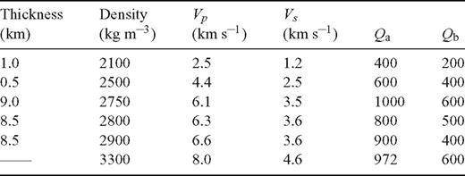
The crustal model used in inversion for the focal mechanism. Vp and Vs are P-wave velocity and S-wave velocity, respectively. Qa and Qb are the Q value of P and S waves.
4.2 Focal Mechanism Inversion
Data quality and azimuthal coverage of the stations are important for the inversion for the focal mechanism. Although the CAP method does not require a large number of stations (Tan et al. 2006), relatively better azimuthal station coverage will produce better estimates of the focal mechanism and focal depth. Epicentral distance is another factor that is taken into consideration for choosing the stations: the shorter the path, the smaller the degradation caused by uncertainties in the crustal model. Thus, we attempt to choose near-field GPS stations with good data quality as well as to homogenize the azimuthal distribution as much as possible. The selected high-rate GPS stations are shown by red stars in Fig. 1. Because all of the stations are located north of the epicentre, the azimuthal coverage is far from ideal.
Based on the selected data, a grid search for strike, dip, rake, moment and depth is implemented by the CAP method to obtain the best point-source solution. The search steps for strike, dip and rake angles are all 5°, and the magnitude step is 0.1 magnitude units. By comparing the total misfit from waveform modelling at different depths, we estimated the centroid focal depth to be about 10 km and the best fitting focal mechanism solution is listed in Table 2. The focal mechanisms from the Harvard GCMT project, the Southern California Seismic Network (SCSN), and the USGS are also presented for comparison (Fig. 6). Recently it has come to our attention that Melgar et al. (2012) also estimated the focal mechanism of this earthquake by GPS data. For this reason, we also compare our result with their work. The comparison shows that the focal mechanisms are similar, the biggest difference comes from the large CLVD component. Their fast CMT solution has a 64 per cent CLVD component, which is quite large for a normal tectonic earthquake. In our inversion there is no CLVD component.
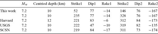
The focal mechanism estimated by using near-field high-rate GPS stations compared with solutions obtained by the Harvard CMT, USGS and SCSN using teleseismic data.
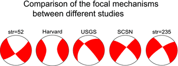
Visual comparison of the focal mechanisms determined here with the Harvard CMT, USGS and SCSN. Two of our focal mechanisms are shown, one with strike angle of 52° (far left-hand side) and the other with strike angle of 235° (far right-hand side).
The dip and rake angles we observe agree fairly well with the teleseismic estimate from the Harvard CMT (ignoring the non-double-couple component), differing only by about 6° and 8°, respectively. There is an apparent discrepancy in the strike angle of about 170°. Fig. 7 shows, however, that there are two minima in strike angle, one near 52° and the other near 235°. Because of the NW–SE strike of the distribution of the aftershocks, the direction of fault rupture should be along NW–SE; thus, the correct focal mechanism of this earthquake should be the conjugate solution. So if the strike, dip and rake angles are taken as 235°, 77° and −14°, respectively, the correct focal mechanism for the earthquake should be 328°, 77°, −167° for strike, dip and rake angles. On the other hand, if 52, 77° and −14° are accepted as the solution, the focal mechanism should be 145°, 76° and −167° for strike, dip and rake angles. The difference between these two focal mechanisms comes from the dip angles. If we select 328° as the strike angle, the fault should dip eastward, while if the strike angle of 145° is chosen, the fault should dip westward. Considering the distribution of the aftershocks, the strong motion pattern of the ground motion (Fig. 1) where more aftershocks are distributed on the east side of the rupture fault and the area with relatively larger ground motion is bigger on the east side of the fault than the west, and the co-seismic rupture model (Wei et al. 2011), then the fault dip to the east should be more reasonable. Therefore, the solution of 235°, 77° and −14° should be in better agreement with the aftershocks distribution and the co-seismic measurements. With this choice, the strike angle is about 14° off from the solution of Harvard CMT, and the focal mechanism is in visually better agreement with the seismic studies as Fig. 6 (str = 235) illustrates. With this choice of strike angle, however, the dip angle changes to about 26°. Thus, the largest difference in our focal mechanism and the teleseismic mechanisms actually is in the dip angle, where our result differs from the Harvard CMT by about 20°. As Fig. 7 illustrates, the dip angle is difficult to observe using near-field data alone under the assumption of an instantaneous point source for such a large earthquake. For dip angles between 50° and 80°, there is little change in misfit. This explains why the dip angle of the main shock in this work is substantially different from the other studies.
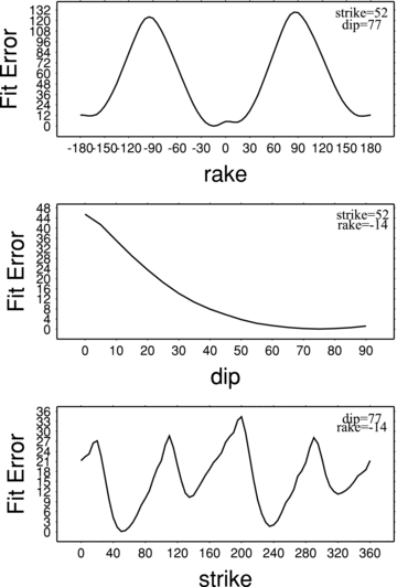
The variation of misfit error with rake, dip and strike angles, from top to bottom, respectively. For misfit as a function of each source parameter, the other two parameters are set to our values presented in Table 2.
From the comparison between observed and synthetic waveforms (Fig. 8) we see that although not all of the time segments are fit equally well, most of the cross-correlation coefficients between the synthetics and the observations are larger than 75 per cent and some are even larger than 90 per cent. This level of misfit indicates that the focal mechanism inversion is acceptable.
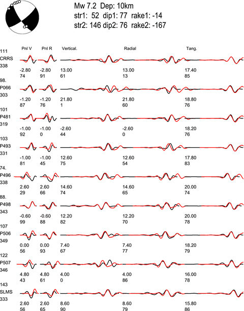
Comparison between the observed and synthetic seismograms of the El Mayor—Cucapah earthquake. The red lines are the synthetic seismograms and the black lines are the observed high-rate GPS displacement waveforms. The frequency band of Pnl waveforms are 0.05–0.2 Hz while for surface waves it is 0.05–0.10 Hz. The top line gives the fit and one fault plane of the earthquake and the beachball shows the focal mechanism of the earthquake. The small circles on the beachball are the P-locations of the stations in which a lower hemisphere projection is used to draw the beachball. The first column gives the azimuth, name and distance to the station. The other five columns are used to compare the synthetic and observed seismograms, from left to right the phases are: vertical component of Pnl (Pnl V), radial component of Pnl (Pnl R), vertical component of surface wave, radial surface wave component and SH wave (Tang.). The synthetic waveform and the observed seismogram are aligned by cross-correlation, the two numbers under the corresponding components are the time shift between the two waveforms and the cross-correlation coefficient between the two waveforms. Detailed information about the method can be found in the article about CAP method (Zhu & Helmberger 1996).
Remaining discrepancies between the focal mechanisms of the USGS, Harvard and this work may be due to several causes. First, the noise level of the high-rate GPS records is higher than that of seismometers, which adds to the ambiguity of the angles of the focal mechanism. Secondly, the observing network we use is very near the earthquake and subtends a narrow range of azimuths. The proximity of the earthquake to the network degrades the assumption that the earthquake is a point source with an instantaneous rupture. In addition, because nearly all of the stations are north of the US-Mexico border and the azimuthal coverage is highly restricted. The geometry of the focal mechanism is, therefore, difficult to resolve. The general similarity between the focal mechanism obtained from near-field high-rate GPS seismology and the mechanisms from USGS, Harvard, and SCSN however, suggests that the GPS observations can be added to regional and teleseismic seismic data in the future for joint analysis.
5 Conclusions and Discussion
We study high-rate GPS records following the El Mayor—Cucapah earthquake within 250 km of the epicentre. These data provide important surface-wave records in the near field where broad-band seismometers either are clipped or are simply not present. Due to complications in the noise recorded on high-rate GPS, signal de-noising techniques that include linear trend removal and wavelet transformation have been developed and applied in this study.
We compare integrated seismometer records (including broad-band seismometers and strong-motion accelerometers in the near field) to the high-rate GPS displacement records. These records are in good agreement for the surface waves in the near field, but beyond about 150 km the high-rate GPS records degrade due to high noise levels believed to be ionospheric in origin.
Combining high-rate GPS in the near field with seismometers at regional to teleseismic distances may lead to more accurate modelling and imaging of the earthquake rupture sequence and source parameters. To test this hypothesis, based on the corrected high-rate GPS records, the focal mechanism of the El Mayor—Cucapah earthquake is inverted using the CAP method. The method reveals a right-lateral strike-slip mechanism with a shallow focal depth of about 10 km. This result is generally consistent with the solutions from the Harvard CMT project, the USGS and the SCSN except for a significant difference in the dip angle. Considering the high noise level of high-rate GPS data, the complexity of the rupture process, and the significantly suboptimal azimuthal coverage of the stations (Fig. 1), the result is seen as confirmation that high-rate GPS observed at near-field stations can be applied in concert with regional and teleseismic seismometers to yield better information about the earthquake rupture properties and parameters. It is, however, strictly not suitable to describe an earthquake as large as the El Mayor—Cucapah earthquake as an instantaneous point source in the near field. Thus, focal mechanisms based on near-field high-rate GPS either alone or in concert with seismic data may be best applied to study small to moderate sized earthquakes.
Acknowledgments
The authors thank the Editor, Jeannot Trampert, and an anonymous reviewer for insightful comments that have improved this manuscript. We also thank Dr Xiaogang Hu at the Institute of Geodesy and Geophysics, CAS for his help on the wavelet transform. We acknowledge EarthScope and its sponsor, the National Science Foundation, and the Center for Engineering Strong Motion Data for providing the data used in this study. This work was joint supported by NSFC grant 40974034, CAS grant kzcx2-yw-142, and NSFC grant (41174086, 41021003).
References
