


Summary
An iterative finite element time-domain (FETD) method has been developed for simulating transient electromagnetic fields in 3-D diffusive earth media and has been verified through comparisons with analytic and finite-difference time-domain solutions. The adaptive time step doubling (ATSD) method plays an important role in reducing solution run-time by allowing large time steps in late time when high-frequency electric fields are increasingly attenuated in the Earth. We demonstrate that for the ATSD method to work effectively, the conductivity of the air and a drop tolerance of a preconditioner should be carefully selected. The conductivity of the air should not be too large for accurate simulations but also not too small for avoiding ill conditioning that results in error amplification in the ATSD method. A proper drop tolerance keeps the eigenvalues of the preconditioned FETD matrices clustered when a time step size is successively doubled during the ATSD processes, resulting in the convergence of iterative solutions with the reasonable number of iterations. A rule of thumb for determining the conductivity of the air and the drop tolerance has been presented. We also present the simultaneous multiple-sources modelling (SM2) approach. The SM2 approach simultaneously advances the electric fields excited by multiple individual sources in a single time stepping loop. This approach allows multiple sources to share the same preconditioner in the time stepping loop and improves the simulation efficiency per a survey line.
Introduction
Transient electromagnetic (TEM) methods have been widely used in a wide range of geophysical research such as deep crustal studies (e.g. Hördt et al. 1992; Hördt et al. 2002), energy explorations (e.g. Strack 1992), environmental investigations (e.g. Auken et al. 2006) and geothermal explorations (e.g. Árnason et al. 2010). Interpretations of TEM data in complex geological environments increasingly resort to multidimensional inverse modelling. Because forward modelling is a major numerical bottleneck for the inverse modelling, it is important to develop efficient and accurate forward modelling algorithms.
Introduced by Yee (1966) in electrical engineering, finite-difference time-domain (FDTD) methods have become one of the standard tools used to simulate TEM fields in geophysics. Their popularity is mainly based on the fact that FDTD methods are relatively easy to implement, easy to use and can provide reasonably accurate solutions over a wide range of geophysics problems. For example, Goldman & Stoyer (1983) present 2-D finite-difference modelling of TEM fields in simplified axially symmetric earth media. Wang & Hohmann (1993) develop a 3-D FDTD algorithm that advances TEM fields in time using an explicit time stepping approach. Commer & Newman (2004) introduce the parallel version of Wang & Hohmann (1993) along with new algorithmic features such as parallel upward continuation procedures and parallel time stepping. The parallel version has been embedded to a 3-D TEM inversion algorithm (Newman & Commer 2005).
Despite their popularity, the 3-D FDTD methods also have well known disadvantages. For example, their explicit time stepping approach requires small time step sizes to satisfy stability conditions especially when there are large conductivity contrasts. To overcome this issue, Haber et al. (2004) use an unconditionally stable implicit time discretization scheme in their finite volume approach (we also employ an implicit time discretization scheme in this paper). Besides, in FDTD modelling, complex geological structures such as seafloor bathymetry, reservoirs and salt domes need to be approximated by small stair steps when the structures do not confirm to rectangular cells. Therefore, this approximation approach can quickly increase FDTD problem sizes; FDTD problems resulting from realistic 3-D earth models are usually solved in massively parallel computing environments (Commer & Newman 2004; Newman & Commer 2005; Commer et al. 2008). Furthermore, such stair steps can introduce discretization errors into numerical modelling results especially when sources and receivers are placed on or very close to the complex surface described by the stair steps.
To avoid the disadvantages of FDTD methods, finite element time-domain (FETD) methods can be considered an alternative. In contrast to FDTD methods, FETD methods are based on unstructured meshes that allow precise representations of arbitrarily irregular topography and complex geological structures in efficient and accurate ways. There have been two major approaches to implement FETD methods. One approach is to inverse Fourier transform the finite element frequency-domain solutions into the time domain (Everett & Edwards 1992; Börner et al. 2008). The other approach is to directly compute FETD solutions in the time domain by advancing EM fields (Lee et al. 1997; Um et al. 2010). The former has been popular in geophysics literature because of its efficiency, but Um et al. (2010) has also demonstrated that it is possible to efficiently advance diffusive EM fields directly in the time domain (1) by reusing the Cholesky factorization (Saad 2003) results and (2) by adaptively increasing a time step size. For convenience, in this paper, we call the FETD method of Um et al. (2010) the direct FETD method, where direct means that the solution is obtained by the back and forward substitution method after a system matrix of the FETD method is decomposed by the Cholesky factorization.
Although Um et al. (2010) presents the efficient FETD method computed directly in the time domain, the FETD method can have numerical difficulties especially for very large-scale problems (e.g. a number of unknowns more than a million on a workstation). For example, as the FETD method employs the Cholesky factorization, the storage requirement for the factorization is at least several ten times larger than that for a corresponding FETD system matrix because of fill-ins. Furthermore, at every time step, the direct FETD method requires back and forward substitution to advance the EM fields. Although several parallel back and forward substitution algorithms have been proposed, their nature is basically serial and is not well suited for parallel computation (Golub & Van Loan 1996).
In this paper, we present an iterative solver version of the FETD method and examine its numerical characteristics. By using an iterative solver, the Cholesky factorization is replaced by the incomplete Cholesky preconditioner. A short summary about the Cholesky factorization and the incomplete Cholesky preconditioner can be found in Appendix. Therefore, as will be shown in this paper, the iterative FETD method requires much smaller storage requirements than the direct one. Furthermore, the back and forward substitution are replaced by matrix-vector multiplication operations in the iterative solver. Unlike back and forward substitution, matrix-vector multiplication can be efficiently parallelized (Golub & Van Loan 1996). Although this paper is not about the parallel implementation of the iterative FETD method, it is important to develop the serial FETD method such that it can be efficiently mapped onto parallel computer platforms for future development.
The remainder of this paper is organized as follows. First, we briefly review the FETD formulation of the electric field diffusion equation and the divergence-free condition. Next, we describe efficient iterative FETD solution strategies in terms of adaptive time step control and reuse of a preconditioner. We also introduce the simultaneous multiple-sources modelling (SM2) approach that makes it possible to simultaneously advance the electric fields excited by multiple individual sources in a single time stepping loop. We follow this by verifying the accuracy of the iterative FETD method through comparison with analytic and FDTD solutions for toy problems. Next, we examine the effects of the conductivity of the air on the iterative FETD method by comparing its accuracy and performance against the analytic and direct FETD method. We also present the performance analysis of the iterative FETD method as a function of a drop tolerance of the preconditioner and propose a rule of thumb for choosing a drop tolerance for a given earth model. Finally, to demonstrate the modelling capability of the iterative FETD method, we simulate EM responses to complex seabed models derived from Society of Exploration Geophysicists (SEG) salt model (Aminzadeh et al. 1997) and present the performance analysis with and without SM2 approach. Through this paper, we also comment on the possibility of the efficient parallel implementation of the presented serial iterative FETD method.
Review on Fetd Formulation
 ,
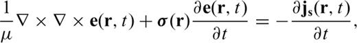
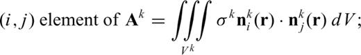
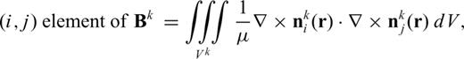
,  are the magnetic permeability, the 3 × 3 electric conductivity tensor and the electric current source, respectively. Note that,
  within the Earth is assumed to be constant and set to that of free space. As shown in Um et al. (2010), the development of the weak statement of eq. (1) requires the multiplication of eq. (1) by the first-order edge elements,
  (Nédélec 1980, 1986; Jin 2002), following by the integration over the volume of the computational domain V.
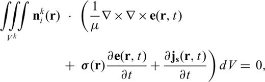
 used in eq. (2) is also chosen as the basis set, the electric field is expanded as
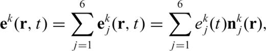
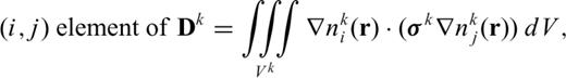
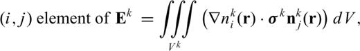
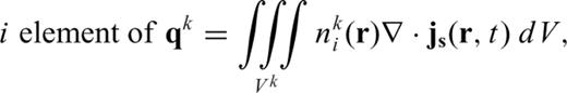
 is the unknown amplitude of the electric field on edge j of the kth element that will be determined by solving a system of FETD equations. Substituting eq. (3) into eq. (2) provides the following system of first-order ordinary differential equations:
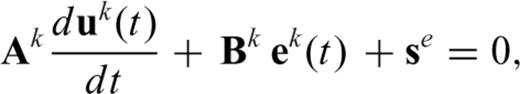
Note that, eq. (9) is the FETD formulation for the kth tetrahedral element. When systems of FETD equations derived from individual elements are assembled into a single large system of FETD equations (i.e. the global version of eq. 9), the superscript k is dropped. The resulting global system matrix is symmetric positive definite (SPD). Therefore, we can use the conjugate gradient (CG) method (Hestenes & Stiefel 1952; Barrett et al. 1994) with an incomplete Cholesky preconditioner (Golub & Van Loan 1996; Saad 2003).
 , which is added to e to satisfy the divergence-free condition by cancelling its gradient component (Smith 1996; Newman & Alumbaugh 2002):
 (Jin 2002) and its subsequent integration over the volume of the computational domain V generates
 used in eq. (11) is also chosen as the basis set for
  , the potential is expanded as
 is the potential of jth node of the kth tetrahedral element.
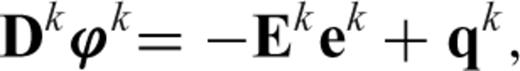

As the final note, eq. (13) is also used to determine the initial value of eq. (9). In this case, ek of the right-hand side of eq. (13) is set to a zero vector. Thus, eq. (13) reduces to a finite element direct-current equation developed in Bing & Greenhalgh (2001) and Um et al. (2010).
Efficient Fetd Solution Strategies
So far, we have developed the systems of FE equations for the electric field diffusion equation and the divergence-free condition. In this section, we describe their efficient solution procedures. In FETD solution procedures, the most computationally expensive part is to advance the solution to eq. (9) in time because it needs to be solved at every time step. To alleviate the computational burden, we exploit the fact that the left-hand side matrix of eq. (9) is time-invariant with a constant Δt. Therefore, for a given Δt, an incomplete Cholesky preconditioner (Appendix) for eq. (9) is computed only once and is repeatedly used inside a time stepping loop. Once time stepping starts, the previous solution is used as an initial guess for the solution at the next time step. On the other hand, as the high-frequency components of the electric fields are more rapidly attenuated in time, we can take increasingly larger Δt and thus, can advance the solution quickly without affecting the accuracy. Therefore, we can change Δt as a strategy for a more efficient solution.
Regarding Δt, we do not determine an optimal Δt at every time step but attempt to double Δt every n time steps, where n is an input parameter. This adaptive time step doubling (ATSD) method effectively prevents unnecessarily small changes of Δt that entail recalculating the preconditioner for eq. (9). At every n time steps,  of eq. (9) is computed twice using both Δt and 2Δt. Then, the difference between the two solutions is compared. If (1) the difference is smaller than a prescribed tolerance and (2) the number of iterations required for convergence with 2Δt is smaller than two times that required for convergence with Δt, then 2Δt is accepted as a new Δt. If either of the two conditions is not satisfied, we reject the new time step 2Δt and continue using Δt. However, the preconditioner for 2Δt is stored for future use as long as memory is available. For brevity, in this paper, we call this approach the ATSD method (Um et al. 2010).
In contrast to eq. (9), the system matrix of eq. (13) is time-invariant. Therefore, after an incomplete Cholesky preconditioner for eq. (13) is computed, it is repeatedly used. Note that the size of the system matrix of eq. (13) is (the number of internal nodes)2 in V, whereas that of eq. (9) is (the number of internal edges)2. Therefore, the system matrix of eq. (13) is relatively small. As a result, the storage requirement for the preconditioner of eq. (13) is insignificant. As a side note, matrix E of eq. (13) is also time-invariant and thus is evaluated only once.
Based on our numerical experiments, the divergence-free condition of eq. (13) does not need to be implemented at every iteration of the main CG solution processes (i.e. eq. 9). Instead, it is sufficient to implement the condition at every m CG iterations, where m is an input parameter for forward modelling. The parameter is empirically determined and varies according to not only a modelling problem but also the quality of a preconditioner. However, when a preconditioner for eq. (9) is sufficiently accurate such that the ATSD method can work effectively as will be presented later, we have found that the CG solution of eq. (9) is accurate enough without explicitly implementing eq. (13). Therefore, our iterative FETD method includes divergence-free condition routines for completeness, but the routines are not frequently used for modelling examples given in this paper. In short, the primary computational cost of the iterative FETD method is (1) to construct a series of preconditioners for eq. (9) with multiple Δt and (2) to perform matrix-vector multiplication operations during CG solution to eq. (9).
To further improve the computational efficiency of the iterative FETD method, we introduce the SM2 approach. In this approach, we design a single FE mesh that can accommodate multiple source positions along a survey line. Then, the single FE mesh is used to simulate the electric fields excited by each source. In this case, at a given Δt, the system matrix of eq. (9) is the same for all sources, whereas the right-hand side of eq. (9) is different with a different source. Accordingly, we can advance the electric fields excited by each source in a single time stepping loop where each source shares the same incomplete Cholesky preconditioner. In other words, inside the time stepping loop, the SM2 approach has an additional source loop in which each source uses the same preconditioner. The effectiveness of the SM2 approach will be demonstrated later.
Accuracy and Performance of Iterative Fetd Method
To verify the accuracy of the iterative FETD method and demonstrate its performance, we compare the iterative FETD solutions with analytic and 3-D FDTD (Commer & Newman 2004) solutions. We implement the FETD method using MATLAB and simulate the controlled-source EM (CSEM) method over homogeneous seafloor and simple 3-D reservoir models. Unless stated otherwise, the presented CSEM models are simulated without explicitly implementing the divergence-free condition. COMSOL Multiphysics 3.5a (COMSOL 2008) is used to discretize these toy models. The simulations presented in this section are carried out on 2.6 GHz Opteron single core with 16 GB memory.
Homogeneous seabed model
We simulate CSEM responses to a homogeneous seafloor model that consists of an infinitely thick air layer, a 400 m thick sea water layer and an infinitely thick seabed (Fig. 1). A 250-m-long x-oriented electric dipole source is placed 50 m above the seafloor. The dipole source generates a step-off waveform. Eight receivers are placed on the seafloor at 1 km spacing along the positive x-axis and another eight receivers along the positive y-axis. The length of the receivers is set to 10 m. The conductivity values of the sea water and the seabed are set to 3.33 S m−1 and 1.43 S m−1, respectively. The conductivity value of the air is set to 10−4 S m−1. In our experience, our FETD method can produce accurate solutions when the air is at least 3 ∼ 4 orders of magnitude more resistive than a medium interfacing with the air. However, if the air is 8 ∼ 9 orders of magnitude more resistive than the medium, the system matrix becomes extremely ill conditioned, resulting in inaccurate solutions. The detailed discussion about the conductivity of the air is presented in the next section.
The x–z section (Y = 0 m) of the 3-D homogeneous seafloor model. The black horizontal arrow is an electric dipole source directed along the x-axis. Its centre is placed at (0 m, 0 m, 350 m).
The boundaries of the model are extended 100 km from its centre to eliminate artificial boundary effects at the receiver positions. As a rule of thumb for making the boundary effects negligible, we set the size of a computational domain to be at least 10 times larger than the maximum source–receiver offset. To discretize such a large model economically, we grow the tetrahedral elements at factors ranging from 1.5 to 2.0 towards the computational boundaries. The model is discretized into 108 540 tetrahedral elements, resulting in 125 883 unknowns for eq. (9).
Fig. 2 shows the cross-sectional view of the FE mesh used for the model at y = 0. The mesh is fine near the source to support high-frequency contents early in time but gradually grows away from the source. The growth rate is empirically determined but is usually less than a factor of 2 from one edge to the next. In addition, because we want to simulate the electric fields measured by 10 m long dipoles, the mesh is also fine near the receivers. In other words, the FETD discretization requires fine meshes around not only the source but also receivers. This is an important difference in the discretization between FETD and FDTD. Note also that inside the sea water layer, tetrahedral elements are restricted from growing rapidly in the x- and y-directions to prevent their aspect ratios from being too small. Consequently, a rather large number of tetrahedral elements are required to discretize the sea water layer.
A cross-sectional view (Y = 0 m) of the 3-D FE mesh used for the homogeneous seafloor shown in Fig. 1. In (a) and (b), the air–sea water interface is coloured as blue and the seafloor red. In (a), the green-coloured line segment above the centre of the seafloor is a 250 m long electric dipole source, and the three shorter green-coloured line segments are the seafloor receivers.
The FETD and analytical solutions show good agreement at selected receivers (Fig. 3). As time stepping continues, errors gradually increase, because of the error migration from early to late time but remains within acceptable levels (<5.0 per cent). Fig. 4 shows the performance of the iterative FETD method with and without the ATSD method. As shown in Fig. 4(a), the ATSD method drastically reduces the number of time steps required to complete the simulation especially when time stepping processes need to continue until late time (e.g. a few time seconds). The ATSD method results in stair-step increase in the solution run-time (Fig. 4b). The increase corresponds to the computational cost of a new preconditioner with a doubled Δt. In the early time, the larger Δt is not accepted because of the presence of high-frequency electric fields. Therefore, in the early time, the ATSD method decreases the performance of the FETD method. However, as the diffusion continues, the ATSD method effectively compensates the extra computational cost because of the new preconditioners by quickly advancing the solutions with larger Δt.
The inline and broadside CSEM responses (Ex) for selected detector positions over the model shown in Fig. 1. (a) The inline electric field responses. (b) The percentage difference between the analytic solutions and the FETD solutions shown in (a). (c) The broadside electric fields responses. (d) The percentage difference between the analytic solutions and the FETD solutions shown in (c).
The performance analysis of the FETD method with and without the ATSD method. (a) Δt versus time and (b) solution run-time versus time.
Seabed model with three-dimensional hydrocarbon reservoir
Next, we simulate marine CSEM responses over a 3-D hydrocarbon reservoir whose conductivity is set to 10−2 S m−1 (Fig. 5). Six receivers are placed on the seafloor with 1 km spacing along the x-axis. The other model and simulation parameters are kept the same as in the previous model. The inline CSEM responses over the reservoir are simulated using both the FETD method and the FDTD method (Commer & Newman 2004) for verification purposes.
The cross-sectional view of the 3-D hydrocarbon reservoir model. The size of the reservoir is 4 × 4 × 0.1 km in x, y and z directions, respectively.
The FDTD model consists of 89 × 79 × 82 grid cells in the x-, y- and z-directions with the computational domain boundaries at 50 km from the centre of the model, resulting in 3 459 252 unknowns. In contrast, with the boundaries of the FETD model extended to 100 km from its centre, we discretize the model into 81 984 tetrahedral elements, resulting in 94 848 unknowns. The comparison of the unknowns between the FDTD and FETD models illustrates an advantage of unstructured FETD meshes over structured FDTD grids.
The simulation results from the methods are plotted in Fig. 6 and show overall good agreement. As a side note, the percentage errors between the two solutions are not provided in this example because the two solutions do not output the electric fields at same outputting points on the time axis. In other words, the FETD method adaptively doubles its time step size over time. At a given time, the FDTD method also dynamically chooses the largest possible time step size that satisfies its CFL condition to speed up its time stepping processes.
The inline CSEM responses at (4 km, 0 km, 1 km), (5 km, 0 km, 1 km) and (6 km, 0 km, 1 km) over the model shown in Fig. 5. (a) Ex. (b) Ez.
Effects of Conductivity of the Air on Iterative Fetd Method
Next, we investigate the effects of the conductivity of the air on the iterative FETD solutions by comparing them with analytic and direct FETD solutions (Um et al. 2010). The goal of this section is threefold. First, we examine the impact of an infinitesimal conductivity of the air on the ATSD method. Secondly, we compare the robustness of the iterative FETD method with that of the direct FETD method over a wide range of the conductivity of the air. Finally, we propose a rule of thumb for choosing a proper drop tolerance of the preconditioner that is closely related to the conductivity of the air as will be demonstrated below.
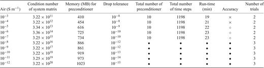
Using both the iterative FETD method and the direct FETD method, we simulate CSEM responses to a layered earth model that consists of a lower half-space (the Earth) and an upper half-space (air). The conductivity of the Earth is fixed at 0.1 S m−1, but that of the air varies from 10−3 to 10−12 S m−1. A 250-m-long x-oriented electric dipole is placed at the centre of the model. The model is discretized into 146 199 tetrahedral elements. Simulation characteristics are summarized in Table 1 for the direct FETD method and Table 2 for the iterative FETD method. CSEM responses are also plotted at selected receiver positions in Fig. 7.
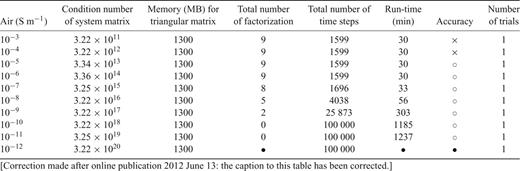
A summary of the direct FETD simulations with various air conductivities. When a direct FETD simulation fails due to numerical instability (i.e. blow-up), the unavailable information is denoted as •. In the seventh column, × and ○ denote inaccurate and accurate solutions, respectively. The innaccurate solutions result from insufficient contrast of the conductivity between the air and the Earth surface. Note that accurate solutions mean that their errors are less than 5 per cent with respect to analytic solutions.
A summary of the iterative FETD simulations with various air conductivities. Symbols are the same as in Table 1.
Effects of the conductivity of the air on the iterative FETD method. The electric field responses (Ex) at three receiver positions (x = 0.5, 1.0 and 1.5 km) along the x-axis are plotted. The conductivity of the air varies from (a) 10−4 S m−1 to (i) 10−12 S m−1 on the log scale. The iterative FETD solutions are not plotted with the conductivity of the air smaller than 10−5 S m−1.
First, we examine Table 1 for the direct FETD method. The one-norm condition numbers of the system matrices of the smallest Δt increase as the conductivity of the air decreases. Note that the conductivity of the air is one and only variable in this numerical experiment. Thus, the increase of the condition number is a direct result of the change of the conductivity of the air. It is noteworthy that the inverse of the conductivity of the air (i.e. the resistivity of the air) is inversely proportional to the condition number on the logarithmic scale. Large conductivities of the air (e.g. 10−3∼ 10−4 S m−1) result in small condition numbers. However, in this case, the air layer becomes very lossy compared with the real air layer (i.e. zero conductivity). As a result, the direct FETD solutions do not agree with the analytical solutions (Fig. 7a). For the next seven conductivities of the air (i.e. 10−5 through 10−11 S m−1), our numerical modelling experiments agree well with the analytic solutions. With the smallest conductivity of the air (i.e. 10−12 S m−1), the FETD solutions diverge at around 0.2 s (Fig. 7i), because round-off errors start to be amplified without control (i.e. blow-up) because of the extreme ill conditioning.
Note that the direct FETD method produces accurate solutions with very low conductivities (e.g. 10−11 S m−1) of the air where the electric fields are in the wave regime. This observation would be counterintuitive as eq. (1) does not include the displacement term. The paradox is explained by the fact that the second term of the left-hand side in eq. (1) becomes negligible when the conductivity is very low. In this case, eq. (1) reduces to Laplace equation. Thus, the finite velocity of the electric field in the real air is replaced by the infinite velocity (Goldman et al. 1985). However, this non-physical aspect does not produce inaccurate solutions for typical EM geophysical modelling because a maximum source–receiver offset is much shorter than the wavelength of the EM field in the real air (e.g. 3 × 10³∼ 3 × 10⁷ km for a frequency range of 0.01–100 Hz). As a result, the FETD method can handle a very low conductivity of the air.
At this point, it is instructive to compare the minimum contrast between the air and the surface conductivity for accurate solutions among different numerical methods. Hördt & Müller (2000) and Commer et al. (2006) report that the contrast of 1:100 would be a reasonable choice for ensuring both accurate solutions and reasonable convergence. The contrast of 1:1000 would result in slow or non-convergence. The contrast of 1:10 would make sounding curves be significantly different from the corresponding analytical solutions especially at early times. In contrast, the numerical modelling experiments presented here show that the FETD method requires at least the contrast of 1:104 between the air and the earth surface. When the direct FETD method is used, the upper limit of the contrast is given as 1:1010. In short, the direct FETD method is relatively insensitive to a large contrast of conductivities in a computational domain.
The total number of time steps required for the direct FETD solution increases quickly as the conductivity of the air decreases below 10−7 S m−1. The same is true for the corresponding solution run-times. Indeed, this observation illustrates that the ATSD method does not work effectively when system matrices are too ill conditioned. As discussed in section efficient FETD solution strategies, the ATSD method accepts 2Δt as a new time step for speed-up when the difference in solutions obtained using Δt and 2Δt is smaller than a tolerance because of the EM attenuation. However, when the air is too resistive, differences between the two solutions are primarily controlled not by the attenuation but by the error amplification because of ill conditioning. Consequently, with the conductivity of the air smaller than 10−9 S m−1, the ATSD method does not work at all, although the high-frequency components of the TEM fields are increasingly attenuated in time.
Next, we examine the numerical characteristics of the iterative FETD method by comparing Table 1 (about the direct FETD method) with Table 2 (about the iterative FETD method). In the numerical experiments, the iterative FETD method allows one more time step doubling process during the simulations, resulting in shorter solution run-times. General benefits of the iterative solver over the direct solver also contribute to the shorter run-times. The memory required for storing incomplete Cholesky preconditioners varies according to the preset drop tolerances. For the conductivities of the air that produce accurate solutions, the memory for the preconditioner (Table 2) is about 45–55 per cent of that for the lower triangular matrices obtained from the complete Cholesky factorization (Table 1).
Despite the advantages discussed above, however, the iterative FETD method also has disadvantages. For example, the iterative FETD method is less robust to a wide range of the conductivity of the air compared with the direct FETD method (Table 1 versus Table 2). More importantly, when a drop tolerance was set to 10−6 for a model with an air conductivity of 10−5 S m−1, the CG solver failed to converge after a prescribed maximum number of iterations (i.e. 30). After two trial attempts, we succeeded in finding a proper drop tolerance (10−9) that not only makes the CG solver converge quickly, but also uses a reasonable amount of memory (Table 2). However, when the conductivity of the air is set smaller than 10−7 S m−1, we were unable to find such a drop tolerance after four trials and discontinued the tests.
Resorting to trial and error for finding a proper drop tolerance is an obvious drawback of the iterative FETD method. However, through extensive modelling experiments, we have found that a good estimate is to set the initial drop tolerance about a few orders of magnitude smaller than the conductivity of the air (i.e. the smallest conductivity in a given computational domain); one can try a smaller drop tolerance for a shorter solution run-time, but this requires more memory. We discuss more on this in the next section. For accurate solutions, the conductivity of the air also needs to be a few orders of magnitude smaller than that of the sea water or the Earth. With such choices, we have succeeded in obtaining accurate FETD solutions with just one or two trials. Throughout the modelling experiments, the iterative FETD method uses about 30–50 per cent of the memory required for the direct FETD method. In short, the conductivity of the air can influence not only the FETD accuracy but also the ATSD method. However, by properly setting the conductivity of the air and a drop tolerance of the preconditioner, the iterative FETD method can compute the EM fields in accurate and efficient ways as shown here.
Impact of Atsd Method on Conditioning of Fetd System Matrix
As demonstrated, the ATSD method is essential to efficiently advance FETD solutions especially in the late time. In this section, by changing Δt and a drop tolerance, we analyse the impact of the ATSD method on conditioning of the system matrix during the EM diffusion and its consequence on the CG convergence. Thus, this section provides a quantitative understanding of the relationship between the CG convergence, a drop tolerance and Δt.
Because the previous models are too large to quickly compute the distribution of their eigenvalues, a small test model is constructed as shown in Fig. 8. To reduce the problem size, the test model is somewhat different from the previous models. First, the test model has only one receiver position at (3 km, 0 km, 2 km). Because small elements are required around receivers, the single source–receiver configuration reduces the problem size. Although the test model has the simplified CSEM configuration, it has representative conductivity for the sea water layer (3.33 S m−1) and the seabed (1.43 S m−1). To ensure numerical stabilities and accuracy, the conductivity of the air is set to 10−3 S m−1. The thickness of the sea water layer is set to 2 km. In contrast to the 400 m thick sea water layer of the previous models, tetrahedral elements in the 2 km thick sea water can grow more rapidly in the x and y directions, reducing the problem size. Accordingly, the model consists of 12 767 elements and has 14 505 unknowns.
The cross-sectional view of a homogeneous seabed model. The single source and receiver are placed at (0 km, 0 km, 1.95 km) and (3 km, 0 km, 2 km), respectively.
The CSEM responses are computed with different drop tolerances ranging from 10−2 to 10−5. The performance analysis is presented in Fig. 9. Note that as discussed in the previous section, a rule of thumb for choosing a proper drop tolerance is to set the drop tolerance a few orders of magnitude smaller than the smallest conductivity (i.e. the conductivity of the air). However, to better understand the impacts of a less accurate preconditioner on the ATSD method, the analysis includes a drop tolerance (i.e. 10−2) even larger than the largest conductivity value (i.e. 10−3 S m−1).
Performance analysis of the iterative FETD method with four drop tolerances. (a) The number of iterations required for convergence at selected time axis points. Note that the CG solver does not converge with the drop tolerance of 10−2 in late time. (b) The history of Δt with four drop tolerances during the diffusion. (c) The accumulated number of time steps with four drop tolerances during the diffusion. (d) The accumulated run-time of the iterative FETD method with four drop tolerances.
When the least accurate preconditioner with the drop tolerance of 10−2 is used, the number of iterations for convergence suddenly increases in late time (Fig. 9a). Furthermore, after around 5 s, the time step size is no longer doubled (Fig. 9b). This is because the number of iterations for convergence with 2Δt becomes larger than twice that required for convergence with Δt. As a result, the time step doubling process does not work anymore after 5 s; the solution run-time quickly increases (Fig. 9d). More importantly, the resulting FETD solutions are inaccurate especially in late time because of non-convergence. However, we still manage to obtain the accurate solutions by activating the divergence-free condition routines and specifying a large maximum number of main CG iterations (e.g. 2000). As a side note, the implementation rate of the divergence-free condition, m is set to 5. However, in this case, the solution run-time is about 103 min, which is considerably long compared with the run-times with more accurate preconditioners shown in Fig. 9(d). This modelling example illustrates that rather than to use inaccurate cheap preconditioners along with the divergence-free condition, it is more practical to use somewhat accurate preconditioners that make the ATSD method work effectively.
As the drop tolerance reduces from 10−2 to 10−4, the increase of the time step makes little impact on the number of iterations for convergence. The ATSD method also works efficiently, reducing the solution run-time. When the drop tolerance reduces from 10−4 to 10−5, the FETD performance does not improve much. To explain the observation above, we first examine the impact of Δt on the system matrix before preconditioning. To do so, the eigenvalue distribution of the system matrix is plotted as a function of Δt (Fig. 10b). As Δt is successively doubled, small and intermediate eigenvalues gradually increase (Fig. 10b). In contrast, large eigenvalues do not change. Thus, the condition number just slightly decreases with increasing Δt (Fig. 10a). In short, the system matrix before preconditioning does not significantly change with different Δt.
(a) The condition number of the FETD system matrix as a function of Δt before preconditioning. (b) The eigenvalue distribution of the FETD system matrix as a function of Δt before preconditioning.
Next, we examine the impact of increasing Δt on the preconditioned system matrix. First, we start with preconditioners with the largest drop tolerance, 10−2. The eigenvalue distribution of the preconditioned FETD system matrices is plotted in Fig. 11. Fig. 12 shows the corresponding condition numbers as a function of Δt (the blue line). When the smallest Δt (i.e. 2·10−3) is used for the system matrix, the eigenvalues of the preconditioned system matrix are clustered well near (1,0) as shown in Fig. 11(a). Therefore, a small condition number is read from Fig. 12. The number of iterations for convergence is also small (Fig. 9a). However, as Δt is successively doubled, the eigenvalues become less clustered (Figs 11d–f). The corresponding condition numbers also quickly increase with Δt (Fig. 12). As a result, the convergence rate quickly deteriorates (Fig. 9a). Because of this reason, the preconditioner with the drop tolerance of 10−2 does not make the ATSD method work effectively.
The eigenvalue distribution of the preconditioned FETD system matrix at selected time step sizes with the drop tolerance of 10−2.
The condition number of the preconditioned FETD system matrix as a function of Δt and as a function of a drop tolerance (varying from 10−2 to 10−5).
The same analysis procedures are repeated with the drop tolerance of 10−4 that is an order of magnitude smaller than the smallest conductivity and thus meets the rule of thumb for a choosing the drop tolerance. The eigenvalue distribution of the preconditioned system matrix is plotted as shown in Fig. 13. Compared with the previous example (Fig. 11), the eigenvalue distribution is more compactly clustered at around (1,0). The increase of the Δt insignificantly changes the distribution of the eigenvalues. Therefore, the condition numbers of the preconditioned matrices remain close to 1 (the black line in Fig. 12). Accordingly, regardless of Δt, the solutions converge consistently just after a few iterations (Fig. 9a).
The eigenvalue distribution of the preconditioned FETD system matrix at selected time step sizes with the drop tolerance of 10−4.
Finally, we investigate the number of non-zeros of the preconditioner as a function of Δt and the drop tolerance (Fig. 14). Note that the number of non-zeros is a yardstick to measure the size of the preconditioner. The number of non-zeros of the preconditioners increases with Δt. Therefore, at a given drop tolerance, the preconditioner that is computed with the largest Δt eventually determines the memory requirement. As shown in Fig. 14, the memory requirement of a preconditioner that meets the rule of thumb for choosing a drop tolerance is about 3 ∼ 4 times that of the system matrix. As a side note, the memory requirement for the complete Cholesky factorization is 11 times that of the system matrix.
The required memory for a preconditioner as a function of Δt and as a function of a drop tolerance varying from 10−2 to 10−5. Note that, nnz stands for the number of non-zeros in a matrix. The required memory for a preconditioner is measured by a ratio of the nnz of the preconditioner to that of the FETD system matrix.
So far, we have analysed the performance of the ATSD method by relating a drop tolerance of the preconditioner to the eigenvalue distribution after preconditioning. In short, successive doubling of Δt tends to increase the condition number of a preconditioned system matrix and thus, decrease the convergence rate. However, when a sufficiently accurate preconditioner is used, the eigenvalues of the preconditioned matrix remains close to (1,0) through successive time step doubling processes, ensuring the fast convergence.
SM2 Approach
In this section, we simulate CSEM responses to a 3-D seabed model that has complex bathymetry, salt and reservoir structures and demonstrate the SM2 approach. Fig. 15 shows the cross-section of central FETD meshes for the seabed model. Its bathymetry and salt structure resemble those of the SEG salt model (Aminzadeh et al. 1997). The seabed model also has a disk-shaped hydrocarbon reservoir whose thickness and radius are 100 m and 2.5 km, respectively. The sea water, the seabed, the salt and the reservoir are set to 3.33, 1.43 and 10−2 S m−1, respectively.
A central portion of the FETD meshes for the complex 3-D seabed model. The red line segments above the seafloor indicate HED sources. (a) The FETD mesh for a single HED source placed at x = 3 km. (b) the FETD mesh for the nine HED sources placed at x = 1–9 km.
The CSEM survey line consists of nine horizontal electric-dipole source positions from x = 1 to 9 km. In a traditional modelling approach, we prepare each FETD mesh for each source position and simulate CSEM responses at each source position. For example, Fig. 15(a) shows the FETD mesh where a single source is placed at x = 3 km. In contrast, the SM2 approach uses a single FETD mesh that accommodates all nine source positions (Fig. 15b) and advances the solution of each source in a single time stepping loop. On average, the FETD mesh with a single source has about 242 767 unknowns, whereas the FETD mesh with the nine sources has 270 622 unknowns. Such small increase in the number of unknowns was possible because seafloor receivers already require small elements along the survey line on the seafloor. Therefore, placing eight more sources 50 m above the seafloor does not critically increase the number of unknowns.
In this paper, we do not intend to present the interpretation analysis of CSEM responses to the seafloor model, but instead focus on the performance analysis of the SM2 approach. For the interpretation analysis, a reader is referred to Um (2011) and Um et al. (2012). Fig. 16 compares the evolution of Δt in the traditional and SM2 approaches at each source position. To ensure the accuracy of the solution, the SM2 approach advances the solution with the smallest Δt from the nine source positions. Therefore, Δt of the SM2 approach never exceeds that of the traditional approach. However, as the SM2 approach enables the nine sources to share the same preconditioner for a given Δt, this benefit outweighs the computational cost related to the smallest Δt. Fig. 17 compares the solution run-time in the traditional and SM2 approaches at each source position. It takes about 7.1 hr for the SM2 approach to simultaneously simulate the nine sources. In contrast, it takes about 1.9 hr for the traditional approach to simulate a single source. Note that the difference in the two solution run-times mainly originates from extra matrix-vector multiplication operations that the CG solver entails in the SM2 approach. However, when we consider the total run-time for simulating the nine sources, the SM2 approach is 2.5 times faster than the traditional approach.
The comparison of the Δt evolution in the traditional single-source modelling approach (blue) and the SM2 approach (red). The nine source positions shown in Fig. 15(b) are considered in (a)–(i).
The comparison of run-time in the traditional single-source modelling approach (blue) and the SM2 approach (red). The nine source positions shown in Fig. 15(b) are considered in (a)–(i).
At this point, it is instructive to consider the parallel computing aspects of the SM2 approach. It is well known that the computation of the incomplete Cholesky preconditioner has poor parallel efficiency (Barrett et al. 1994). In contrast, the matrix-vector multiplication operation is easy to be parallelized and is effectively scalable (Golub & Van Loan 1996). Accordingly, the SM2 approach that shares the preconditioner and requires extra matrix-vector multiplication operations is well suited to parallel computing environments. We expect that the SM2 approach would further improve overall efficiency of the iterative FETD method on parallel computer architectures. We currently develop parallel versions of the iterative FETD method along with the SM2 approach and the ATSD method, and will investigate their performance.
Conclusion
A new iterative FETD method has been developed for simulating EM responses to 3-D earth models. Unlike existing FETD methods, our FETD method iteratively computes the EM fields directly in the time domain. We demonstrate that the direct time-domain computation can be fast and efficient. The ATSD method enables the iterative FETD method to take increasingly large time step sizes over time and reduce the total number of time stepping processes, speeding up the solution processes. For the ATSD method to work efficiently, the conductivity of the air should not be too small. In this case, the ill conditioning of the FETD system matrix prevents the ATSD method from working in an intended way.
A proper choice of a drop tolerance of the preconditioner is also important. When the drop tolerance is set several orders of magnitude smaller than the conductivity of the least conductive medium (i.e. the air), the eigenvalues of the preconditioned system matrices keep clustered during the successive time step doubling processes. As a result, the CG solutions converge within the reasonable number of iterations at each time step. We also demonstrate that the SM2 approach improves the overall efficiency of the FETD method by making multiple sources share the same preconditioner for a given Δt. In short, the ATSD method and SM2 approach are effective algorithm-driven speed-up techniques for simulating EM diffusion directly in the time domain. In our ongoing research, as the hardware-driven speed-up techniques, we consider implementing the presented iterative FETD method on different parallel computing architectures and analysing their performance.
Acknowledgments
This work was carried out at Lawrence Berkeley National Laboratory. Um was supported by Early Career Development Grants from Earth Sciences Division. Editor Dr. Gary Egbert and reviewers Drs. Antje Franke and Souvik Mukherjee provided helpful suggestions for improving this manuscript.
Appendix
Appendix: Complete and Incomplete Cholesky Factorization
In this appendix, we provide readers with a short introduction to complete and incomplete Cholesky factorization. One can find various pseudo-codes and in-depth discussions about the factorizations in Saad (2003).
This is the complete Cholesky factorization. This factorization is used in the direct solver version of the FETD algorithm (Um et al. 2010). For example, the FETD algorithm directly solves Ax = b,by first implementing eq. (A1), then solving UTy = b for y and finally solving Ux = y for x. Although, a system matrix arising from finite element applications to EM problems is sparse, the triangular matrix resulting from the factorization is usually dense because fill-ins occur during the factorization. Therefore, although a reordering scheme (e.g. Karypis & Kumar 1999) is employed, a storage requirement for U is typically several orders of magnitude larger than that for matrix A.
The incomplete Cholesky factorization essentially resembles the complete Cholesky factorization. However, during the factorization, the incomplete Cholesky factorization drops elements of U that are smaller than a prescribed tolerance (i.e. drop tolerance). Thus, U reduces to Uinc ; error matrix E is introduced.
The incomplete Cholesky factorization has been widely used as a preconditioner for the CG method in EM problems (e.g. Jin 2002; Zhu & Cangellaris 2006). A small drop tolerance value generally produces a more accurate preconditioner than a large drop tolerance, but requires a larger storage for Uinc. For example, when a drop tolerance value is set to zero, the incomplete Cholesky factorization reduces to the complete one. Following Saad (2003), a pseudo-code of the incomplete Cholesky factorization used in this paper is given as

In line 6, an element row(k) is dropped (i.e. replaced by zero) if it is less than the relative tolerance  obtained by multiplying the drop tolerance by the two-norm of the ith row of matrix A.
References
