


Summary
The properties of the plate interface region influence plate coupling and rupture behaviour during large earthquakes. Plate coupling varies greatly along the Hikurangi subduction zone in the southern half of the North Island, New Zealand, and heterogeneous material properties can be examined with the well-recorded seismicity. For this study, we have used a modified velocity inversion to incorporate earthquake differential times from selected groups of distributed earthquakes, which improves the spatial resolution of features in the lower crust, and sharpens velocity gradients. Data are selected from temporary deployments and the permanent GeoNet network, which has expanded in the last decade. The resulting 3-D velocity model shows that the overlying plate exhibits patterns related to geologic terranes. The Rakaia terrane has low Vp/Vs and high Vp, and is spatially related to the zone of strong plate coupling. Seismicity occurs throughout the overlying plate, and extends to the plate interface without a lower crustal aseismic zone. The Wairarapa–Waewaepa fault zone may form the updip limit of strong coupling in future plate interface earthquakes. The crust of the subducting plate is characterized by abundant seismicity and is bounded by strong velocity gradients. Low-velocity zones above the plate interface are indicated from 30 to 50km depth. Seismic velocities near the plate interface show an excellent correlation with the distribution of plate coupling, and provide insight into what controls such coupling. The plate interface has the highest Vp/Vs (>1.85) and sharpest Vp/Vs gradient in the region of strongest coupling, consistent with the suggestion that strong coupling is related to the inability of fluid to cross the plate interface. In regions of recurrent slow slip, Vp/Vs is still high, but the gradient of Vp/Vs near the plate interface is much broader, suggesting movement of fluid across the plate interface. The area of deep slow slip corresponds to the most extensive high Vp/Vs mantle region above the slab.
Introduction
This study examines the Hikurangi subduction zone in the southern half of the North Island of New Zealand, which is a region where the plate coupling varies greatly (Wallace et al. 2009). Our goal is to determine the material properties near the plate interface, in the overlying plate and in the subducted slab. The properties of this region influence the rupture behaviour (coupling) of the plate interface in large earthquakes. Such properties may be comparable to other subduction zones such as northeastern Japan where heterogeneous plate coupling has also been derived (Suwa et al. 2006). Despite the lack of historical Hikurangi subduction thrust earthquakes, Wallace et al. (2009) infer that the margin may be capable of producing great subduction thrust events as large as Mw≈ 8.2–8.7.
Overlying the shallow plate interface is a long-lived frontal wedge. This consists of imbricate-thrust accreted sediment from both trench-fill and landward erosion, with the oldest (Lower Cretaceous) units at the inboard edge above the plate interface, and up to 7-km thick Neogene–Quaternary sediment at the seaward edge (Lewis & Pettinga 1993; Lee & Begg 2002). Onshore, the continental crust consists of a group of primarily greywacke accreted terranes. This overlying crust experiences active deformation along the North Island dextral fault belt (Fig. 1), as well as through spatially varied uplift and extension. Onshore earthquake hypocentres are well constrained and 3-D velocity and Qp variations within the overlying plate and the subducted slab have been imaged (Eberhart-Phillips et al. 2005; Eberhart-Phillips et al. 2008). These results showed high Vp/Vs and low Qp in the region of weak coupling. The Qp results suggested that overlying plate properties could inhibit fluid flow to the backarc mantle, and further seismicity studies showed that the impermeable terrane prevented fluid from dehydration of the subducted plate from crossing the plate interface (Reyners & Eberhart-Phillips 2009). Improved understanding may come from more detailed study, incorporating data from the expanded permanent seismic network.
Tectonic setting of the southern Hikurangi subduction zone. Red contours show the interseismic coupling coefficient at the plate interface (Wallace et al. 2012), whereas the green contours enclose regions where the total slip in slow slip events at the plate interface has exceeded 50mm since 2002 (Wallace & Beavan 2010). Terranes in the overlying plate are shown coloured, namely: BS, Brook Street; CA, Caples; DM, Dun Mountain; KA, Kaweka; MB, Median Batholith; MO, Morrinsville; PA, Pahau; RA, Rakaia. Faults mapped at the surface are shown as thin lines, with the major fault zones identified, namely: WF, Wairau fault; WMFZ, Wellington–Mohaka fault zone; WWFZ, Wairarapa–Waewaepa fault zone. The arrow shows the velocity of the Pacific Plate relative to the Australian Plate (DeMets et al. 2010). The white line outlines the area shown in Fig. 8. The inset shows the location of the study area on the Pacific/Australian plate boundary: AF, Alpine Fault; HP, Hikurangi Plateau; HT, Hikurangi Trough; KT, Kermadec Trench.
The seismicity near the plate interface extends offshore to where the plate interface is at 10–15km depth. To extend our resolution of the plate interface zone, as well as improve resolution of the overlying plate and subducted slab, we have modified our 3-D velocity inversion program to include differential traveltimes. Got et al. (1994) and Waldhauser et al. (1999) have used differential times to relocate clustered earthquakes. Michelini & Lomax (2004) showed that the accuracy of these double-difference relocations is dependent on the velocity model, and Zhang & Thurber (2003) developed double-difference tomography. For two earthquakes that are close together relative to the distance to a given recording station, the differential time is the difference in the traveltimes of the earthquakes observed at the station, and residuals in the differential time will be primarily related to velocity variations near to the earthquakes, and to variation in the relative hypocentral locations. Offshore plate interface earthquakes have poorly constrained hypocentres because of weak azimuthal coverage, and adding differential time data across them will improve their relative locations and allow offshore earthquakes to better contribute to the velocity model. Onshore, the plate interface earthquakes form a zone at 20–30km depth with sparse seismicity in the overlying crust, leading to vertical smearing of velocity features within the overlying plate. Differential times among these earthquakes may improve the spatial resolution of features in the lower crust region, and sharpen velocity gradients. Also, receiver differential times can be obtained by taking the difference in traveltimes from a given earthquake to two stations that are closely spaced relative to the distance to the earthquake. Use of receiver differential times may improve spatial resolution of the shallow crust.
Method
The use of differential times was put forth and implemented by Waldhauser & Ellsworth (2000) in the program HypoDD, to simultaneously relocate groups of earthquakes. Their foundational study incorporated cross-correlation times of highly clustered earthquakes, some of which had been shown to be repeating earthquakes with identical locations, in the dense northern California seismic network. HypoDD used a 1-D seismic velocity model. Zhang & Thurber (2003) expanded this into a simultaneous velocity-hypocentre inversion program (TomoDD) by incorporating a 3-D seismic velocity model, and for each differential time setting velocity partial derivatives along the ray paths from the two earthquakes to the common station. In an alternate approach, Monteillier et al. (2005) showed that for the purpose of velocity inversion, the ideal differential times come from declustered distributed earthquakes that are not colocated, but rather a small distance apart, relative to the distance to the common station.

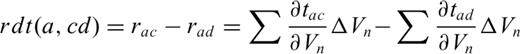
Schematic diagram of receiver differential times (rdt) and earthquake differential times (edt). For earthquake Ea, having traveltime residuals at receivers Rc and Rd, rdt (a,cd) is the difference between the residuals. For earthquakes Ea and Eb, each a having traveltime residual at receiver Re, edt (ab,e) is the difference between the residuals.
The ray paths are calculated with the pseudo-bending routine, with an enlarged suite of initial ray paths (Eberhart-Phillips & Bannister 2010). The portions of the paths close to Rc and Rd will have the most influence on their rdt, whereas distant portions near to Ea will have very similar partial derivatives as their paths are more closely spaced than the gridpoints. An input parameter, edist, gives the maximum distance allowed between edt earthquakes or rdt stations. During set-up of the differential times, edist12 is the distance between earthquake or receiver pairs, paths are only included where the slant distance is more than four times edist12, partial derivatives are set along a distance facray times edist12 and only high-quality arrival times are used for differential times. For our study, edist12 ranged from 3–20km, our grid spacing was 4–12km and we selected a facray of 1.5.
In addition to traditional earthquake and shot data files, a file of earthquake group traveltimes is included. During the location stage of each iteration, the groups are each located by including the differential times to simultaneously locate all the hypocentres in a group with the current 3-D velocity model. There is no assumption that the earthquakes in a group should be collocated, and the calculated hypocentre perturbations are simply those that minimize all the residuals of the group. During the velocity inversion stage of each iteration, the updated group hypocentres are used for traveltime and ray path calculations, but they are fixed like shots, rather than having their hypocentral partial derivatives included through parameter separation as is done for single event earthquakes. This makes the problem tractable, as it is not feasible to do parameter separation for groups of hypocentres, and we wanted to retain the Simul solution method. We tested LSQR for locating earthquake group hypocentres, and found that it did a poorer job with residuals 20–700per cent worse than with SVD. For the edt earthquake groups, both the input traveltime observations and the derived edt data are used, in both the hypocentre and velocity stages of each inversion iteration. During inversion, receiver differential times can be selected. If desired they can be calculated for each single earthquake, and then the set of receiver differential times for each event is included as a shot, separately from the related earthquake.
The velocity solution is obtained by damped least-squares inversion, using LU decomposition as in previous versions of the Simul code. This provides a solution that has few artefacts and stays close to the initial model where there is little resolution. No general smoothing constraints are needed to get a reliable solution. Thus, the only smoothing which comes into the model is that which is inherent in the distribution of the data, and in the distribution of the velocity nodes. The full resolution matrix is computed, allowing the analysis of how the velocity features may be smeared.
Velocity grid approaches
The initial velocity model and the velocity model parametrization are important issues for the model resolution. The initial model influences the location of the sources because hypocentres are dependent on the velocity model. It also influences the velocity perturbations that are computed in the inversion. Our previous work (e.g. Eberhart-Phillips & Bannister 2010) has shown that gradational inversions from coarse grids to regional to fine grids give the most reliable solution. For example, in a test case of a sharp gradient and low-velocity fault zone, with a 1-D initial model, the fault dip was inaccurate and there was strong overshoot of the high-velocity side (Eberhart-Phillips et al. 1995). In gradational inversions, the 3-D model gets progressively more detailed.
With earthquake data, the data coverage is always uneven and various means are used to accommodate this. Automated adaptive grids have been developed by Michelini (1995) and Zhang & Thurber (2006) for the local scale, and on a global scale by Bijwaard et al. (1998) to give reasonable data coverage in regions with little data by having varied size blocks. Another approach is to perform such redesign of model parameter areas or volumes (blocks) outside of the inversion code. This allows expert review and control by the user to avoid problems with arbitrary assignments. For instance, an initial inversion could show that there is a velocity gradient across a region, and it would be preferable to not have the enlarged blocks extend across the gradient as that would lose the ability to resolve the gradient. Within the Simul program, flexible gridding through linking of nodes can accommodate varied size grids related to data distribution (Thurber & Eberhart-Phillips 1999). This is extremely flexible and can link nodes in any sized block, and the velocity perturbation of the block can be assigned to be constant across the block or linear such that the block's master node gets the computed perturbation and the slave nodes get a gradient between master nodes.
The Simul flexible gridding method has been used in several manners. Generally, the approach is to first run an initial inversion with fine grid spacing, and then examine the derivative-weighted sum (DWS), together with the pattern of velocity perturbation to determine node linking. Various automated linking routines can be used to create linked nodes based on the DWS, with input criteria for maximum and minimum combined DWS. In the Southern Alps region of New Zealand (Eberhart-Phillips & Bannister 2002), the P data had better resolution than the S data, and hence the automated DWS linking of nodes resulted in linking within most of the Vp/Vs model, but little linking of Vp above 30km depth. The autolinked pattern was evaluated before using it in the velocity inversion, and additionally large areas offshore were linked in a way to essentially create a 2-D model where there was little data. In the North Island subduction zone, the primary feature, the high-velocity subducted slab, is approximately 2-D. There, an initial model was obtained by linking all the nodes in the along-strike direction to obtain a 2-D model (Reyners et al. 2006). Along the Ryukyu arc, Lin et al. (2004) used flexible gridding with two-scale grids: the master grid had 18km spacing and the fine-scale slave grid had 6km spacing (a third of the master spacing). In areas of high ray path density, the fine-grid nodes were unlinked to become free parameters, thereby allowing recovery of fine-scale structure when possible and reliable smoothed structure where there was lower resolution.
Another issue for velocity grid definition is the influence of specific grid placement because the actual velocity is defined at specific nodes and interpolated between them. Even when the velocity solution is precise for the grid locations, this can result in a bumpy appearance to planar features in the velocity model. Also, for sharp gradients, it can result in overshoot of velocity at the node to give the appropriate velocity nearer to the boundary. Gradational inversions reduce these effects. Averaging of staggered grid results is another method to improve the imaging of continuous features. The staggered grid method for Simul has been implemented by Haberland et al. (2009) for the south-central Chile subduction zone. Several inversion runs are carried out with the same grid spacing, but offsetting the specific grid placement. Then those varied grid results are averaged onto a finer grid that includes all the varied offset grids. This approach gives a reasonable, smooth result on the scale of the fine-grid nodes, which is directly obtained from data that can only resolve larger scale features. It does not specifically penalize velocity gradients, but rather will improve the spatial pattern of velocity gradients. Averaging has also been used successfully with TomoDD by Calo et al. (2011), who averaged results from 15 grids of varied orientation.
The averaging approach can similarly be used in conjunction with the flexible gridding method. There is always some degree of arbitrariness in the assignment of master and slave nodes and specific design of enlarged blocks. Averaging can mitigate the effect of spatial patterns related to placement of enlarged blocks. Grid set-up and autolinking routines can be carried out in several slightly different ways to have a variety of appropriate linking grids with different master nodes and different placement of enlarged blocks. Then velocity inversions can be done with the various linking grids, and the results from those inversions can be averaged together (Eberhart-Phillips et al. 2008). This averaging of linked grid results will give a solution which is appropriate for the data distribution but has fewer arbitrary patterns related to the velocity gridding. Our philosophy towards obtaining 3-D velocity models considers that the inversion program is not a black box, and geophysical models are always non-unique. Thus, the most reliable results may be obtained by the scientist exerting expert control over the process, and evaluating the results from a range of inversions that are deemed appropriate for the given region and data set.
Data
The permanent seismic network in New Zealand has developed over the last 20 years from the time of initial digital instrumentation to a comprehensive network (GeoNet: www.geonet.org.nz; Petersen et al. 2011) with denser station coverage, through a combination of broad-band, short-period and strong-motion stations. There have also been numerous temporary deployments for regional studies, and these data have been incorporated in 3-D velocity studies. The combined results provide a New Zealand (NZ)-wide 3-D velocity model (Eberhart-Phillips et al. 2010). The combined station distribution is shown in Fig. 3. In our study area, most of the additional GeoNet stations were operational by 2008 August, with one being added in 2009 July. We have emphasized the more recent data in our selection process, although we have included older data (from 1990 and later) when it improves the spatial distribution. In this region, temporary networks were deployed in 1990, 1991 and 2001, for both microearthquake recording and active source studies (Eberhart-Phillips et al. 2005; Reyners et al. 2006). For all data, we required at least eight observations and minimum earthquake magnitude of 1.8.
Stations used in the velocity inversion, a combination of permanent GeoNet stations and various temporary arrays. The rectangle shows the study area, with the locations indicated of cross-sections of Fig. 10.
The focus of this study is on the region of the plate interface that is in contact with the crust of the overlying plate, where the deformation processes involve coupling across the plate interface rather than the deeper viscous mantle flow. Thus, we have limited the region for selected edt earthquake groups to the area where the plate interface is shallower than 50km, which is where x > 40km in model coordinates, (Fig. 3). An even distribution and variety of ray path coverage is desirable for velocity inversion, and typically sources are selected to be spatially distributed and well recorded. This is a different goal than HypoDD, where the need is to relocate dense clusters of seismicity. Thus, we aim to select evenly distributed earthquake groups. We use a binning and selection program which splits a region into overlapping boxes, of specified dimension, bins all the available earthquakes into those bins and selects a group from each box for the velocity inversion. The bins have 20per cent overlap so hypocentres can fall into multiple bins, and the selection of a particular hypocentre was limited to three times. The selection parameters are the minimum distance between events, and the minimum and maximum number of events in a group. We used a minimum interevent distance of 3km, and allowed 8–35 earthquakes in each group.
Binning was done at three scales, as shown in Fig. 4 for two depths. The primary bin dimension was 25km, which resulted in 111 groups. The region offshore has fewer earthquakes and no nearby stations, and so there edt data could provide improved resolution in the vicinity of the earthquakes. However, given the sparse seismicity, most of the offshore 25km bins did not return selected groups. Thus, we used a larger dimension of 40km offshore, and obtained 23 additional groups, and left 30 total events within all the unused boxes. The total number of selected earthquakes was 2703 for the 134 groups. These data were used for the first inversion runs. For the finer scale inversions, we additionally selected edt earthquake groups at a smaller size with 12km bins, using the earthquakes that were not included in the previous selection. The 12km bins provided 366 groups, with a total of 3285 hypocentres. The fine-scale inversions incorporated all 500 groups. For each stage of the inversions, a preliminary run was done to enable data evaluation within the edt groups, and the few events that had poorly constrained hypocentres (67), with high non-decreasing rms residuals or large fluctuating changes in hypocentral parameters, were removed.

Groups of earthquakes for differential times were selected from bins at three scales. The primary bin dimension is 25km, with overlap of 20per cent. For sparser seismicity bin dimension was 40km, and for dense seismicity additional bins of 12km (diamonds) were used in the fine-scale inversions. The bin locations are indicated at the bin centre; for example distributions at 20 and 40km depths are shown.
We additionally include standard single-event data for regions where there were too few earthquakes to form groups, and for the area northwest of the binned region so that the model will be consistent with regional data. A distributed set of 453 events for the northwest region was selected from data used in previous studies (Eberhart-Phillips et al. 2010) and recent data (2007 March–2010 June). The deepest selected earthquakes are 100km deep. Another 94 distributed earthquakes were selected from those in unused bins in the binned region. We also included two shots from the 1991 Hikurangi margin refraction profile (Chadwick 1997). In summary, we used 232 549 observations, of which 209 443 were associated with earthquake groups. The observations were composed of 176 014 P traveltimes and 56 535 S–P traveltimes. Within the inversion run, this created 4701 P and 65 S–P rdt data; and 264 131P and 3279 S–P edt data.
Velocity Inversion Application
We incorporate gradational inversions, flexible gridding and averaging in the inversion process for the southern Hikurangi Plate interface (SPI) region. The NZ-wide 3-D velocity model (Eberhart-Phillips et al. 2010) is used as the initial model. With a regional model that covers an area broader than our study area, we can include stations outside of the inversion area without worrying that peripheral artefacts will result. The velocity inversion grid area is shown in Fig. 3. The orientation of the inversion grid was chosen with the y-axis parallel the strike of the subduction zone (040°). The y-axis is positive to the southwest and the x-axis is positive to the southeast. The first SPI inversion (SPI-A; Fig. 5) for the area indicated in Fig. 3, was carried out on the NZ-wide grid to obtain the best model on that grid for the expanded data set before stepping to a finer grid. For comparison, the initial model is shown in Fig. 6(a). This inversion used the selected single event and shot data, and the edt earthquake groups of 25km and 40km dimension. For the edt earthquake groups, both the traveltime residuals and the edt data are minimized. The inversion grids extended to 85km depth, although the regional model extends to 370km depth.
Comparison of gradational velocity inversion results. Left: SPI-A is inversion with expanded data set on the NZ-wide grid. Centre: final model, SPI-D, obtained by very fine-grid inversion, on the averaged model of four different inversions on fine grids. Right: alternate approach, SPI-E, is inversion on very fine grid with NZ-wide as initial model. Cross-sections of Vp and Vp/Vs models, ‘x’ show inversion hypocentres near each cross-section.
For the same cross-sections as Fig. 5, comparison of initial model and perturbations. (a) Initial model for the local inversions is the regional NZ-wide model. (b) Difference between final model (SPI-D) and initial model. (c) Influence of differential times is shown by the difference between the final model (SPI-D) and a model obtained without using edt or rdt data.
The next finer scale inversion (SPI-B) had additional x-grids to have 7km x-grid spacing, and several additional z-grids were added from 30 to 55km depth. This also included the edt earthquake groups of 12-km dimension. In the trench-normal direction, we incorporated staggered grids, such that a similar but staggered inversion (SPI-C) had x-grids offset by 3km from SPI-B. For each of these grids, two different runs were done with flexible gridding and the master nodes were assigned in different ways. Thus, there were four runs with similar grid spacing, which are equally appropriate for fitting the data. These four velocity models were averaged together to give a finely gridded (3km) model (SPI-BC). We want to be certain that the averaged model provides a good fit and also allow the data to adjust it if necessary for fine-scale detail. Hence, SPI-D is a fine-scale run with the averaged model as the initial model. This is our preferred model and is shown in Fig. 5. The total reduction in data variance was 35.5per cent, from the initial NZ-wide model. The perturbation from the NZ-wide model is shown in Fig. 6(b). Most of the reduction (25.5per cent) came in the first inversion (SPI-A), and the moderate grids (SPI-BC) produced about half as much (11.0per cent) additional reduction in data variance. The final fine grid inversion (SPI-D) produced about a tenth (2.2per cent) additional reduction in data variance, yet is an important step to assure that the model averaged to the fine grid is still appropriately fitting the data.
For comparison, a fine-scale inversion (SPI-E) has been done directly from the NZ-wide model, without using flexible gridding or averaging (Fig. 5). Overall the result is similar, but the velocity pattern is bumpier, and the plate interface gradient does not appear as a smooth feature. It is more difficult to interpret, and also it does not fit the data as well. Note that our preferred model (SPI-D) actually has a slightly higher model variance. It is not a smoother model. An element such as a relatively sharp gradient that is continuous over a large distance may visually appear smoother, but it can produce a greater increase in model variance than a bumpy, less well-defined gradient.
To evaluate the influence of the edt data, we also carried out a set of inversions using all the earthquakes that are in the edt groups, but running them as single events without computation of additional edt data, and also not allowing rdt data. A comparison is shown in Fig. 6(c) displaying the difference between SPI-D and the no-edt model, with a contour interval of 0.15kms−1 dVp and 0.015 dVp/Vs. This shows that the edt and rdt data contributed small effects, with very few places having |dVp| > 0.3kms−1. The differences primarily sharpen gradients; particularly in portions near the east coast and offshore, near the overlying plate Moho, above the subducting plate crust and within the subducting plate. For example, the high Vp/Vs in the slab mantle is more clearly separate from the slab crustal high Vp/Vs than without edt data included.
The rdt data primarily influence the shallow crust near the stations, and hence a comparison at 3km depth is shown in Fig. 7. The differences are minor and the patterns are the same. The gradients are sharper with the rdt data, so the fault zones are somewhat better defined and there is slightly higher velocity in the Axial Range relative to the Wanganui Basin.
Influence of receiver differential times at 3km depth. (a) Final model (SPI-D). (b) Model obtained without using edt or rdt data. (c) Difference between (a) and (b).
Results
The 3-D model is shown in map views at 15, 30 and 48km depth in Fig. 8. Hypocentres near each depth section are shown and the lines indicate the limits of resolution. The crust of the overlying plate (Figs 8a and d) exhibits patterns related to terranes, and a change in Vp/Vs across the Wairarapa–Waewaepa fault zone. Lower P-velocity (<6.0kms−1) characterizes the eastern Pahau terrane, although the Rakaia and Kaweka terranes have low Vp/Vs and higher Vp (>6.0kms−1). Low Vp is also associated with the Wanganui Basin. The crust of the subducting plate is associated with abundant seismicity bounded by strong gradients at 30km depth (Figs 8b and e) with patchy high Vp/Vs. The subducted slab mantle is shown at 48km depth (Figs 8c and f) with high Vp (>8.2kms−1) and large areas of high Vp/Vs. Low-velocity zones above the plate interface are indicated in both the 30 and 48km depth sections.
Map views of inversion results for Vp (top) and Vp/Vs (bottom) at depths of 15, 30 and 48km, with white or yellow lines showing limit of good resolution, as represented by SF = 3.5 contour (see Fig. 9), ‘x’ show inversion hypocentres near each depth. Letters A–E indicate features discussed in the text.
This paper focuses on the 3-D velocity results. Locating groups of earthquakes with the addition of edt data across the events may improve the hypocentres, and we have briefly examined that aspect. For comparison, we have located the inversion events in the final velocity model (SPI-D) as single events. The hypocentres are very similar with only a few showing significant differences: 90per cent are within 1km of those with edt data, 99per cent are within 3km and only 0.3per cent have difference greater than 5km.
Resolution
The full resolution matrix is also calculated. Resolution of the fine 3-D model SPI-B is shown in Fig. 9 for the cross-sections in Fig. 10. The resolution matrix describes the distribution of information for each node, such that each row is the averaging vector for a parameter, and is summarized in the spread function (SF; Michelini & McEvilly 1991), which describes how strong and peaked the resolution is for each node. We also illustrate the pattern of image blurring in low-resolution areas by showing contours of the averaging vectors for nodes that have significant smearing. From each row of the resolution matrix, we compute smearing contours where the resolution is 70per cent of the diagonal element (Reyners et al. 1999). Resolution contours are shown only for those nodes which have smearing such that the resolution contour extends beyond an adjacent node. At other nodes, we would expect the spatial averaging to be represented by the grid spacing.
Resolution for the 3-D Vp and Vp/Vs models, for cross-sections, indicated in Fig. 3, showing the spread function and 70per cent smearing contours for nodes that have significant smearing. Inversion hypocentres shown as white dots.
Depth cross-sections of the 3-D Vp (left) and Vp/Vs (right) models, for the same cross-sections as shown for resolution (Fig. 9). Limit of good resolution is shown by white or yellow lines of SF = 3.5 contours, ‘x’ show inversion hypocentres near each cross-section. Mapped location of Caples, Rakaia and Pahau terranes is indicated. Interseismic coupling coefficient (Fig. 1) is labelled for Φ= 0.4, Φ= 0.8 above sections. The strongly coupled locked zone is indicated by solid red or green lines. Regions of slow slip (Fig. 1) are indicated by dashed red or green lines. White dots label the plate interface at 15, 25 and 40km depth. Letters A–E indicate features discussed in the text. Fault zones: W-M Fz, Wellington–Mohaka; W-W Fz, Wairarapa–Waewaepa; Wa F, Wairau; Aw, Awatere. Other labels: W Co, west coast; E Co, east coast; CapeK, Cape Kidnappers; Wang Bas, Wanganui Basin; Sub T, subduction trench.
The reliability of features in the 3-D inversion can be evaluated by combined use of the SF and resolution smearing contours. For low values of the SF (<2.5), the model Vp or Vp/Vs is representative of the volume surrounding a given node—that is, the volume between that node and adjacent nodes. Nodes with moderate SF values (2.5 < SF < 3) have acceptable resolution, but may be averaging a larger volume, and small features may not be imaged or may appear as broad features. Nodes with SF values in the 3–3.75 range have meaningful velocity patterns, but the size of the velocity perturbations may be smaller than actual velocity heterogeneity. Fig. 9 shows the resolution for a fine grid which had 7km grid spacing. The prior run with a coarser grid (SPI-A) had somewhat broader resolution, averaging volumes further offshore. The SF = 3.5 contours from SPI-A are drawn on the cross-sections in Fig. 10. That can be considered the limit of adequate resolution for interpretation.
The Vp model has little smearing in the plate interface region from 15 to 55km depth, having fairly uniform good resolution with SF < 2.2. At the shallowest depths, there is vertical smearing over the upper 8km. The Vp is well resolved by the edt data which require high-quality observations, and relatively few S arrivals have adequate quality for computing edt data. The large part of the plate interface where there is distributed seismicity has excellent resolution with SF < 1, on the grid with node spacing less than 5km. The Vp/Vs has acceptable resolution, but not as good as Vp, and has some smearing in the central area (e.g. Fig. 9g). However, note that the smearing distances are small, 5–10km. Thus, we can interpret patterns of Vp and Vp/Vs in the plate interface region as spatially representative below shallow depths. Offshore as the plate interface shallows above 15km depth, the shallow seismicity provides some resolution but there is lateral smearing and the shallowest offshore area is generally not well sampled. In the overlying plate below 35km depth, there is some vertical and lateral smearing, particularly in Vp/Vs, which may degrade spatial resolution to 10–15km.
In the subducted slab there is good resolution to the depth of the lower band of seismicity, at 50–70km depth. Thus, the low-velocity zones in the slab are adequately resolved for interpretation. In the region of the high-velocity slab at 55km depth, there is reasonable and uniform resolution from y =−408 to −228. Further southwest, the slab resolution is weaker and the less distinct high velocity there may result from poor resolution.
Synthetic model
To further evaluate resolution, a synthetic model was created with some typical subduction zone features. This has sharp boundaries on a fine grid so that the features cannot be obtained exactly, and hence the test inversion allows us to evaluate how well such features are resolved. As shown in Fig. 11 (left), our synthetic model has a slab with high-velocity mantle, and a 12-km-thick crust which has moderately high Vp/Vs. Above 25km depth, there is a thin layer of subducted sediment with low Vp and high Vp/Vs. The overlying plate has a few large regions with differing Vp and Vp/Vs, which could represent terranes, and a narrow vertical low-velocity zone. Where the plate interface is shallower than 20km depth, there are areas of low Vp and very high Vp/Vs. The slab mantle has a section with high Vp/Vs. Synthetic data were created for the same events as the actual data. A 1-D initial model was used for inversion of the synthetic data. First, coarse 2-D and 3-D inversions were done to form a regional model. Then we ran a series of inversions similar to the inversions on the actual data, as the latter had the regional NZ-wide model as the initial model.
Synthetic test model to evaluate smearing and resolution of features. Left panels show synthetic Vp and Vp/Vs for three y-sections, and right panels show the test inversion results.
The slab is imaged well from the synthetic inversions (Fig. 11, right). The crust (6.8–7.0kms−1) is well resolved, especially where there is dense seismicity. The inversion results show a very sharp gradient, from 7.0–8.0kms−1 over a few kilometres, similar to the actual model. East of x = 150, the slab is weakly resolved, as the SF is worse (Fig. 9) and it becomes even harder to image sharp gradients. The velocities of the slab mantle are generally good, being over 8.5kms−1 although the synthetic slab mantle is 8.7–8.8kms−1, although the varied resolution conveys apparent patterns. In the slab mantle below the earthquakes, the retrieved velocities appear overly high, as it spreads the gradient over a broader zone. As seen in map view at 48km depth (Fig. 12e), there are some areas of Vp > 9.25kms−1 that appear patchy. The patchy overshoot of mantle high velocity occurs at nodes below the deepest earthquakes and appears similar to the very high-velocity patch (>9.5kms−1) in the actual inversion (Fig. 8c). Thus, we must discount those highest velocity patches. However, the overall similarity of the actual slab velocities to results from the 8.7–8.8kms−1 synthetic slab shows that actual slab mantle velocity ∼8.8kms−1 may be inferred.
Synthetic test model to evaluate smearing and resolution of features. Upper panels show synthetic Vp and Vp/Vs for three depths, and lower panels show the test inversion results.
The synthetic slab mantle has a 30km wide high Vp/Vs zone (Fig. 12c). The shape and extent of this zone are well resolved, but only a few spots reach the actual high Vp/Vs (1.86), and the eastern extent is limited (Figs 11d and 12f). The synthetic slab crust has high Vp/Vs which is obtained throughout the crust, but is patchier and tends to be smeared vertically (Fig. 11). The crustal high Vp/Vs has become a wider zone, with its central high Vp/Vs systematically shifted to shallower depth, particularly where there are few earthquakes in the overlying plate. Thus, in Figs 11(a) and (b), where there is abundant seismicity (near x = 100–125), the Vp/Vs result is more spatially accurate even though the synthetic model is more complex with a fault zone, eastern shallow high Vp/Vs and a thin very high Vp/Vs zone of subducted sediment.
In the overlying plate, the eastern high Vp/Vs and low Vp area is imaged with appropriate shape for x < 150 (Fig. 11b), and offshore (x > 150) weakly high Vp/Vs is obtained. The synthetic model also had a thin layer of very high Vp/Vs subducted sediment for x > 115, which is imaged in only a few spots. In the crustal area from x = 40–120, the large terrane blocks are imaged with appropriate velocities and smoother boundaries (Fig. 12d). For x < 40, there are a few higher velocity spots, apparently because of vertical smearing of deeper high velocity. The low Vp/Vs feature is imaged with its lowest Vp/Vs in the appropriate location, however it is smeared towards the northwest, and its sharp edges are not possible to image (Figs 11d and f). The synthetic model also has a thin vertical low-velocity zone with moderate Vp/Vs at x = 115 (Fig. 12a). Although the inversion grid is unable to show such a thin feature, there is a broader slightly low-velocity zone in the upper 10km on most sections (Figs 11b, d and f).
In the region of the mantle wedge, the subducted crust is a low-velocity zone. This low-velocity zone is imaged along the whole region (Fig. 12e). The mantle wedge velocities are too high in some sections (Fig. 11b) and too low in others (Fig. 11d). The mantle wedge high Vp is smeared vertically in sections with no overlying plate earthquakes (Fig. 11f). The mantle wedge has a block of high Vp/Vs (Fig. 12c) which is obtained in the correct location and smeared to the southwest as the sharp edge cannot be resolved (Fig. 12f).
To evaluate the influence of the edt and rdt data, we have also done test inversions without the edt and rdt data. The results are not much different, with few places where |dVp| > 0.15kms−1 or |dVp/Vs| > 0.015. Fig. 13 compares the actual inversion, the synthetic inversions and the difference with the edt data for a given cross-section. The similarity with or without the edt data shows that the largest improvement over the regional model comes from using more data on a fine grid with averaging of multiple runs. The dVp plot (Fig. 13e) shows a sharpening of the gradient across the plate interface. There is especially improvement near the east coast and offshore, where there is 0.35kms−1 higher velocity slab and some imaging of the thin subducted sediment layer. The shallowest part of the crustal fault zones is also better imaged, from the rdt data. The high Vp/Vs in the slab mantle is slightly better imaged by the edt data in that it is less smeared and looks more distinct from the crust high Vp/Vs. The high Vp/Vs near the plate interface is slightly narrower with less overshoot of overlying low Vp/Vs. East of x = 120, the high Vp/Vs subducted sediment that ends at the fault is better imaged. Overall, the use of a synthetic model with such sharp gradients and thin zones illustrates how such features may be broadened or smeared by 3-D inversion models.
Comparison of actual model, synthetic model and influence of edt and rdt data for cross-section y =−310. (a) Final model with actual data (SPI-D). (b) Synthetic model. (c) Test inversion. (d) Test inversion without edt or rdt data. (e) Difference between (c) and (d).
Plate interface
The plate interface can be defined at the top of the smoothly curved region of upper-plane seismicity in the slab, in the cross-sections in Fig. 10. There is also overlying plate seismicity extending all the way to the plate interface, where the interface is shallower than 25km. Thus, along this portion of the Hikurangi margin, there is no aseismic zone above the plate interface.
The plate interface is characterized by a strong velocity gradient along the sections in Fig. 10, with the gradient appearing sharpest where there is accretionary wedge material, in the southeastern parts of sections y =−408 to −310 (Figs 10a–c). Northwest of the Wairarapa–Waewaepa fault zone in the region of overlying greywacke terranes, the plate interface is approximately at the 6.5kms−1 contour, where the overlying material has Vp > 5.5kms−1. To the southeast, where there are overlying forearc sediments with Vp < 5.5kms−1, the plate interface is at about the 5.8kms−1 contour. The 3-D model has a more complex image of the plate interface at about 25km depth on the y =−348 to −310 sections where the Wellington–Mohaka fault zone intersects the plate interface (Figs 10b and c), with slightly reduced Vp in the top of the slab. The upper plane of seismicity in the slab is a smooth continuous feature across to the east coast, and is clearly distinct from the seismicity associated with the fault zones in the overlying plate. In most sections, there is a low-velocity zone above the plate interface, where the plate interface is 30–50km deep, particularly in the southwest from y =−198 to −105 (Figs 10f–h).
The plate interface has moderately high Vp/Vs at all depths, and the high Vp/Vs extends to the surface in the reverse-fault tectonic regime in the southeastern area. The high Vp/Vs is patchy (Fig. 8e), and the highest Vp/Vs (>1.85, ‘D’) and sharpest Vp/Vs gradient are at y =−198 where there is the strongest coupling (Fig. 10f). In the southernmost section (Fig. 10h), there is a change to having slightly high Vp/Vs above the plate interface and slightly low Vp/Vs below it.
Discussion
Structure of the overlying plate
The overlying plate crust comprises a series of terranes described by Mortimer (2004) and Adams et al. (2009), as illustrated in Fig. 1 and labelled above the cross-sections in Fig. 10. The Rakaia and Caples terranes formed in a Permian–Triassic accretionary wedge. The Rakaia terrane contains quartzofeldspathic greywacke metasedimentary rocks, with the stratigraphically lower Caples terrane being more andesitic. The Rakaia terrane experienced extended tectonism and metamorphism in the latest Triassic to late Jurassic interval. The early Jurassic Kaweka terrane, located immediately north of the Rakaia terrane, had a similar southern sedimentary source. The Jurassic Morrinsville terrane, located west of the Rakaia and Kaweka terranes, contains volcaniclastic sandstones from a different northern sediment source, and has experienced only low-grade metamorphism. The youngest terrane, the Cretaceous Pahau terrane, is trenchward of the Rakaia and Kaweka terranes and contains volcaniclastic sandstones. Thus, the primary difference among the terranes is the degree of metamorphism, with the Rakaia terrane undergoing the most metamorphism (Mortimer 2004; Adams et al. 2009).
The locations of key terranes are shown above the velocity cross-sections (Fig. 10). In the southern half of our study area, the Rakaia terrane is centrally located above the subducting slab (blue in Figs 10e–g). In the mapped geology (Fig. 1), the adjacent Morrinsville terrane gradually tapers to a narrow zone so that in the southernmost sections, the western basement rocks are Caples terrane; approaching the South Island, the Morrinsville and Rakaia terranes are truncated by the Wairau fault (Fig. 10h). In our 3-D velocity results, the Axial Range and greywacke terranes exhibit internal complexity and structure that varies along the margin. The Rakaia and Kaweka terranes have fairly uniform velocity of 5.8–6.2kms−1, generally low Vp/Vs and show vertical lower velocity zones that may be related to faults. The low Vp/Vs is consistent with schist. Given the results of our synthetic tests (i.e. comparing Figs 10f and g with Figs 11c–f), it is likely that the region of lowest Vp/Vs is restricted to the Rakaia terrane. This is consistent with it having undergone the most metamorphism. The Morrinsville terrane has similar Vp to the Rakaia terrane above 20km depth, but has higher velocity at 23km depth, which could be related to fragments of mafic oceanic crust, as interpreted from high Qp (Eberhart-Phillips et al. 2005). The southwestern sections (Figs 10e–h) have a region of higher velocity material northwest of x = 75, which is associated with the Caples terrane.
The Pahau terrane is distinctive with lower Vp (6.0kms−1) and relatively high Vp/Vs, indicative of high fluid pressure (Figs 8a and d). It also has more seismicity compared to the Rakaia terrane, which is characterized by a lack of seismicity. Such ongoing background seismicity indicates a material with abundant microfractures, in contrast to the strong, older and highly metamorphosed Rakaia terrane. The southeastern sedimentary forearc accretionary wedge has distinctive low Vp and high Vp/Vs, and a sharp velocity gradient at its base (Figs 10a and b). However, its internal structure is not evident in the 3-D velocity image.
This study focuses on the shallow part of the subduction zone where the overlying plate is largely crustal. Our 3-D inversion method does not define a specific Moho discontinuity for the overlying plate, although the velocity gradients may be associated with velocity boundaries, and the Moho has been generally estimated from the 7.5kms−1 contour. In a broader scale study of the central North Island, Reyners et al. (2006) inferred a crustal thickness greater than 40km southwest of y =−348, and slightly thinner to the northeast where it is approximately 35km thick. A similar pattern is seen in the finer scale model in this paper. In the series of cross-sections in Fig. 10, the furthest northeast (y =−408, −348) indicate mantle velocities at shallower depth. For reference a dot on each cross-section shows the plate interface at 40km depth. It is evident that the Rakaia and Pahau accretionary wedge terranes in the North Island have no associated underlying mantle.
Our 3-D inversion also provides more detail on the mantle properties above the slab, with varying low-velocity zones in this region. This velocity reduction most likely represents alteration of mantle properties rather than deflection of the crust/mantle boundary. In this region, serpentinization of the mantle occurs, with the extent of serpentinization related to the amount of fluid released from dehydration of the underlying slab. Such serpentinization is associated with reduced Vp and high Vp/Vs (Hyndman & Peacock 2003).
Thus, along most of the study region there is an ∼15km wide low-velocity zone adjacent to the slab, which becomes a broad low (E) from y =−300 to −225 (Fig. 8c). Its Vp/Vs properties (Fig. 8f) show even more variation, with a large region (C) of high Vp/Vs (>1.825) associated with the broad low Vp. The inferred areas of most extensive serpentinization also have seismicity in the base of the overlying crust, centred at about 35km depth (Figs 10d–f). Such a concentration of seismicity in the lower crust, restricted along the strike of the subduction zone, has also been seen in previous compilations of 3-D relocated earthquakes (e.g. Reyners et al. 2011; their fig. 3). It suggests that the mantle wedge in this region is not only serpentinized, but also fluid-rich and permeable (Peacock et al. 2011), with fluids leaving the wedge and triggering earthquakes in the base of the overlying crust. Why is this only happening in a restricted region along-strike? A plausible explanation was suggested by Reyners & Eberhart-Phillips (2009) to explain the suppression of deeper earthquakes in the subducted slab further updip. They proposed that here the Rakaia terrane provides an impermeable plate interface, which inhibits dehydration embrittlement (and the resulting earthquakes) deeper in the underlying slab. Studies of the kinetics of antigorite dehydration (Miller et al. 2003; Perrillat et al. 2005) have demonstrated that fluid overpressures impede such dehydration. Thus, fluid overpressures extending into the deeper slab beneath the impermeable Rakaia terrane may retard antigorite serpentinite dehydration reactions there. So downdip of the Rakaia terrane, there may be an abnormal amount of fluid release, due to the catch-up of dehydration reactions.
Structure of the subducted slab
Our improved tomography has provided finer detail on the structure of the subducted slab than that provided by earlier tomographic inversions (e.g. Eberhart-Phillips et al. 2005, 2010). The subducted slab exhibits generally high Vp, and Vp contours within the slab are parallel to the plate interface and are fairly smooth (Fig. 10). Apparent bumpiness in the derived velocity structure is more likely to represent crustal velocity variations than complexity within the slab. The image changes where the slab intersects the Moho of the forearc, where the plate interface is about 40km deep. At that depth, the top of the slab forms a low-velocity zone between the overlying mantle and the deeper slab, such that there is a boundary in Vp/Vs with slightly high Vp/Vs above and slightly low Vp/Vs below (e.g. Figs 10b and g). The deeper slab has varied Vp/Vs and tends to exhibit moderately high Vp/Vs, over 1.78, for the region southeast (updip) of x = 85km (Fig. 8f). Overall, the Vp/Vs image shows a change downdip to moderately low Vp/Vs at about x = 80, but the pattern is varied with some sections (e.g. y =−198; Fig. 10f) showing particularly low Vp/Vs, less than 1.675.
The main feature that we are imaging in the slab is the subducted Hikurangi Plateau (Reyners et al. 2011). This plateau was originally part of the Ontong Java Plateau, the largest oceanic plateau on Earth. In our study region, the plateau has subducted to greater than 100km depth (Reyners et al. 2011), well beyond the northwestern edge of our tomography grid. The plateau is ca. 35km thick, and its lower crust has transformed to eclogite. It is this eclogitic layer which produces the very high Vp of >8.5kms−1 that we see in the slab, centred ca. 30km below the plate interface (Fig. 10). The synthetic model had uniformly high Vp (8.7–8.8kms−1) in the slab mantle. The test inversion obtained high velocity, but with a gradient such that overly high Vp (>9.2kms−1) occurred at nodes below the mantle earthquakes (Fig. 13). Thus, we do not want to overinterpret the deep high Vp (>9.2kms−1) in our results, and we infer that the actual high Vp slab mantle may have more uniform Vp < 9kms−1.
The results also show low Vp features in the slab mantle, which are not reproduced in the synthetic inversions (Figs 13a and c; x = 75). For instance, there is a large patch with lower Vp and low Vp/Vs at y =−408 to −348 (Figs 10a and b). There are also smaller patches with reduced Vp at y =−228, −198 and −141 which form a linear zone of lower Vp within the slab, and appear to go through the upper 35km of the slab. These lower Vp regions tend to have low Vp/Vs, although the low Vp/Vs areas are larger than the near-vertical low Vp zones. The synthetic inversion results had patchy velocity in the slab, although the actual low Vp variations are larger than found in the synthetic results (compare Figs 10e and 11d). Similar lower velocity zones have been observed in other subducted slabs, and these may reflect hydrated faults that formed before subduction (e.g. Nakajima et al. 2011). Given that this zone is along-strike, it may reflect bending-related tensional faulting formed at the outer-trench slope during the current subduction episode. Alternatively, it may reflect pre-existing structure within the Hikurangi Plateau, as the southeastern plateau is dominated by a northeastern volcanic grain (Davy et al. 2008). However, because the resolution is uneven, we cannot be certain that the slab low-velocity zone is realistic, and further investigation would be helpful.
Vp/Vs in the subducted slab is highest (>1.85) beneath the updip part of the most strongly coupled part of the plate interface (Figs 10e and f). This result is consistent with the suggestion of Reyners & Eberhart-Phillips (2009) that the plate interface in this region is sealed, with fluid produced by dehydration reactions within the slab unable to cross the plate interface. Such sealing will lead to high fluid pore pressures within the slab, and thus produce the high Vp/Vs that we observe (e.g. Audet et al. 2009). Similarly, the marked reduction in Vp/Vs beneath the downdip end of the most strongly coupled part of the plate interface (Figs 10e and f), suggests that here the plate interface becomes permeable, with fluids free to leave the slab. This will lower fluid pressures within the slab and reduce Vp/Vs.
Structure near the plate interface and its relationship to plate coupling
Structure near the plate interface revealed by our inversion shows an excellent correlation with the distribution of plate coupling, and provides insight into the controlling factors for such coupling. The distribution of the interseismic coupling coefficient at the plate interface determined from GPS inversions (Wallace et al. 2012) is shown in Fig. 1, together with the regions of recurrent slow slip that lie at the downdip edge of the coupled part of the plate interface (Wallace & Beavan 2010). Note that cumulative slow slip since 2002 has a maximum of >300mm in each of the slow slip regions shown.
The deepest region of strong plate coupling occurs beneath the centre of the Rakaia terrane near the y =−198 cross-section (Fig. 10f). On this section, we have added a line segment along the plate interface marking the region where the interseismic coupling coefficient is >0.4. Of all the depth sections, this has the sharpest gradient in Vp/Vs across the plate interface, and the most concentrated seismicity in the top of the subducted slab. The strong gradient is because of both low Vp/Vs in the overlying plate and high Vp/Vs within and below the slab crustal seismicity. These observations are consistent with the inference of Reyners & Eberhart-Phillips (2009) that the strong interseismic coupling is related to the inability of dehydration-released fluid to cross the plate interface, resulting in high fluid pore pressure immediately below the plate interface. This inference is based on the correlation between the distribution of strong interseismic coupling at the plate interface derived from GPS, the distribution of small earthquakes in both plates and 3-D crustal structure from tomographic inversions. The impermeable nature of the highly metamorphosed Rakaia terrane, suggests it plays a major part in forming this permeability seal at the plate interface. The low Vp/Vs is representative of the Rakaia terrane, and the high Vp/Vs may relate to high-fluid pressure. The synthetic inversion had high Vp/Vs throughout the slab crust and it was imaged across the region, generally centred above the plate interface. In contrast, the actual results generally do not show as high Vp/Vs as the synthetic results. For example, considering the y =−348 section (Figs 10b and 11b), the actual results have only slightly high Vp/Vs for the region downdip of the WWFZ. The particularly high Vp/Vs determined for the slab crust in the y =−198 section is thus unique in our results and not an artefact.
Fine structure of the interplate thrust itself may also play a role. A layer of subducted sediment, 1–2km thick with Vp < 4kms−1, has been inferred from a seismic refraction experiment along the east coast of the southern North Island (along x = 125; Chadwick 1997). We cannot discriminate the presence of such a thin layer overlying the subducted plate with our tomography. Amplitude modelling suggests this layer of sediment thins towards the northeast along-strike (Chadwick 1997), in the direction of decreased coupling. So, the thicker sediment in the southernmost North Island may contribute to a more effective seal at the plate interface.
At the downdip edge of the strongly coupled part of the plate interface, which corresponds to the regions of recurrent slow slip, the gradient in Vp/Vs near the interface is much broader, suggesting movement of fluid into the overlying plate (Fig. 10). In map view, the region of highest Vp/Vs (>1.83) in the deeper overlying plate nicely tracks the regions of slow slip, being centred at (130, −350; label A) at 15km depth (Fig. 8d), (50, −330; label B) at 30km depth (Fig. 8e) and (30, −275 and southwestward; label C) at 48km depth (Fig. 8f). Below approximately 40km depth, the mantle of the overlying plate interacts with the subducting plate, and the seismic properties vary. It has especially high Vp/Vs (C) and low Vp (Fig. 8c, label E) in the region downdip of the strongly coupled part of the plate interface, and where there is more seismicity in the lower crust. The relationship of high Vp/Vs and slow slip suggests that high fluid pore pressures are probably a necessary condition for slow slip (e.g. Gomberg et al. 2010). But our results suggest that such high fluid pore pressures may be more correlated with slow slip when they extend into the overlying plate.
Shallower slow slip also appears related to abundant fluid flux. In the northeastern sections (y =−408, −348; Figs 10a and b) only weak coupling (Φ < 0.2) is inferred over the whole plate interface, and most of the plate interface has experienced recurrent slow slip (Fry et al. 2011). The sedimentary forearc accretionary wedge (southeast of the Pahau) has distinctive low Vp and high Vp/Vs. The underlying slab mantle has abundant dehydration seismicity. Above 40km depth, the entire plate interface has high Vp/Vs indicating high-fluid pressure, and overlying high Vp/Vs suggests permeable material allowing fluid flux across the plate interface. Yet below 40km depth in the northeastern sections, the mantle wedge does not exhibit low Vp or high Vp/Vs.
Our tomography results also provide information on the likely updip extent of strong plate coupling. Note that one cannot learn about the updip extent of plate locking from geodetic data alone (McCaffrey 2002). The sharp gradient in Vp/Vs across the plate interface and the concentrated seismicity in the top of the subducted slab in the region of strongest coupling dies out updip near the boundary between the Rakaia and the younger Pahau terranes (e.g. Fig. 10f). Also, the Pahau terrane is characterized by a lower Vp and higher Vp/Vs than the Rakaia terrane, particularly in its trenchward side (e.g. Figs 8a and d). These results suggest that this terrane is permeable, and allows fluid to flux across the plate interface. There is also a sharp change in b-value at the Pahau/Rakia boundary, with high b-value in the Pahau, suggestive of abundant fractures, while low b-value in the Rakaia terrane relates to rigid material (Montuori et al. 2010). The moderately high Vp/Vs and high b-value in the Pahau terrane suggest it is overpressured, in line with borehole results (Darby & Funnell 2001). So following the argument that strong coupling occurs where fluid cannot cross the plate interface, then the Rakaia/Pahau terrane boundary provides a first-order estimate of the updip limit of strong plate coupling. Note that southwest of y =−348, both the relatively high Vp and low Vp/Vs in the lower part of the overlying plate between the Wellington–Mohaka and Wairarapa–Waewaepa fault zones suggest that the Rakaia terrane may extend at depth to the location of the Wairarapa–Waewaepa fault zone. This finding is consistent with the Permian–Triassic Rakaia terrane having been a backstop for the accretionary wedge associated with Cretaceous subduction at the edge of Gondwana, which is now the Pahau terrane. So, for estimating the updip limit of strong coupling in the southern North Island when determining the hazard from future large plate interface earthquakes, the Wairarapa–Waewaepa fault zone should be used. As a cautionary note, the ruptures of recent great earthquakes, Mw≥ 8.8 (Tohoku: Shao & Ji 2011; Maule: Vigny et al. 2011) have propagated updip through the shallow velocity-strengthening region. Dynamic rupture models could be tested with the Hikurangi Plate interface properties and crustal fault interaction.
The Rakaia terrane is truncated between the North and South Island (Fig. 1), and in the northern South Island the seismogenic part of the plate interface is overlain by Pahau terrane. There is a narrower region of subduction coupling as the deformation transitions to a system of strike-slip faults. The terrane here is characterized by relatively low Vp (<6.5kms−1) and moderately high Vp/Vs (Fig. 10h), again suggesting that fluid crosses the plate interface and leads to overpressures in the terrane. The downdip limit of strong coupling also shallows significantly in this region, consistent with the idea that fluid crossing the plate interface weakens coupling (Reyners & Eberhart-Phillips 2009).
The relationship between crustal faults and the plate interface
Seismicity occurs throughout the overlying plate, and extends to the plate interface without a lower crustal aseismic zone. Thus, there is no apparent brittle-ductile transition. Most of the deeper seismicity is in a zone underlying the Wairarapa–Waewaepa fault zone. This broad zone of distributed seismicity is about 15km wide, narrows towards the surface and is associated with low-velocity zones in the upper 10km on nearly all the y-sections in Fig. 10 (e.g. Fig. 10d). The Wellington–Mohaka fault zone also has associated low-velocity zones along the southwestern sections, y =−228 to −141 (Figs 10e–g). In northeastern sections, y =−408 to −310 (Figs 10a–c), it forms a boundary with higher velocity on the northwest and higher Vp/Vs on the southeast.
It is clear from our Vp images that the Wellington–Mohaka fault zone has played a major role in the uplift of the Axial Range of the North Island. From y =−408 to −228, Vp is relatively high (>6.0kms−1) at shallow depth to the northwest of the fault (Figs 10a–e), suggesting uplift of the ranges has been produced by thrusting on the fault. The shape of the uplifted Vp = 6.0kms−1 contour changes from near-vertical in the northeast (Fig. 10a) to northwest-dipping in the southwest (Figs 10d and e), consistent with the fault becoming more listric towards the southwest. Given that the surface trace of the fault moves progressively updip on the plate interface as one moves southwestward (Fig. 1), the fault meets the plate interface near the downdip end of the strongly coupled zone on sections y =−272 to −228 (Figs 10d and e). This makes sense mechanically, as it is difficult to sustain active faulting which bottoms out at a locked portion of the plate interface. Our interpretation of the role of the fault is consistent with geological data. Nicol & Beavan (2003) have shown that high strains in the overlying plate are concentrated near the downdip end of the contemporary locked zone. Furthermore, this downdip end has been approximately stable over a period of at least 2.5–5 Ma, sufficient time to uplift the Axial Range.
In the southernmost North Island (Figs 10f and g), tomographic evidence for thrusting on the Wellington Fault is not obvious, and the fault becomes predominantly strike-slip (e.g. Beanland 1995). Here, the fault lies close to the Wairarapa–Waewaepa fault zone, at the inferred updip end of the region of strong coupling. Again, this is a mechanically favourable place for faulting to develop in the upper plate. It should be noted that both the Wellington–Mohaka and Wairarapa–Waewaepa fault zones are not revealed by seismicity lineations. Rather, small earthquake activity in the overlying plate is more diagnostic of terranes, with the Morrinsville and Pahau terranes having much more small earthquake activity than the intervening Rakaia terrane (e.g. Figs 10e and f).
Conclusions
The modified velocity inversion includes earthquake differential times to improve imaging regions near earthquake groups, such as the plate interface region. Preferred results are obtained with progressively finer scale inversions, flexible gridding and averaging in the inversion process.
The subducting oceanic crust is defined by relatively sharp Vp gradients and moderately high Vp/Vs. Underlying high Vp (∼8.8kms−1) in the slab is consistent with the presence of eclogite in the lowermost portion of the 35km thick Hikurangi Plateau. Synthetic tests show that it is difficult to interpret additional structure such as faults in the slab mantle.
The overlying plate influences interseismic plate coupling. The region of strong plate coupling that extends to 40km depth appears related to the oldest most metamorphosed terrane which has low Vp/Vs characteristic of relatively impermeable schist. In addition, the underlying oceanic crust has its highest Vp/Vs, consistent with high fluid pore pressure. We infer that the impermeable terrane inhibits slab fluid release, and that the lack of fluid flux is related to strong coupling.
The Wairarapa–Waewaepa fault zone forms a boundary in Vp/Vs with high Vp/Vs trenchward. It has a broad zone of distributed seismicity extending to the plate interface. The Wairarapa–Waewaepa fault zone thus may influence aspects of subduction thrust rupture behaviour and perhaps may form the updip limit of strong coupling in future plate interface earthquakes.
High fluid pore pressures may be most correlated with slow slip when they extend across the plate interface into the overlying plate, indicative of abundant fluid flux. The area of deep slow slip may correspond to the most extensive high Vp/Vs mantle region above the slab. This region may be serpentinized and fluid-rich with overlying fluid-triggered earthquakes. In the shallower slow slip region, abundant fluid flux is also inferred from the forearc accretionary wedge with distinctive low Vp and high Vp/Vs, and underlying slab mantle seismicity.
Acknowledgments
This work was supported by the Marsden Fund administered by the Royal Society of New Zealand, and the New Zealand Ministry of Science and Innovation. The manuscript has benefited from comments by Stephen Bannister and Bill Fry, and two anonymous reviewers.
References
