Estimation of the anisotropy parameters of transversely isotropic shales with a tilted symmetry axis

Summary

Introduction

In any practical attempt to determine the type and the magnitude of elastic anisotropy in a natural rock sample, its homogeneity needs to be assumed and therefore experimentally verified (Lucet & Zinszner 1992). A representative volume element must exist and be smaller than the sample size. If this is not the case, no self-consistent elastic symmetry would emerge from the measurement of several independent ultrasonic wave velocities. In other words, the dependence of elastic wave velocities with angles of propagation would display no trend but should appear random. In the following discussion, homogeneity of the rock samples is assumed based on qualitative analysis of the measured ultrasonic wave velocities. The aim is therefore to recover the magnitude of elastic anisotropy based on the quantitative analysis of the experimental data set.

Because of preferred orientation of platy clay particles, the elastic behaviour of shales often displays a transversely isotropic (hexagonal) symmetry with a rotationally invariant axis perpendicular to the bedding plane. Computation of P wave anisotropy parameters (ɛ and δ) of shales from ultrasonic measurements on a single specimen traditionally rely on a very limited number of independent measurements, for instance along, normal to, and at 45° to the bedding plane (Jones & Wang 1981; Lo et al. 1986; Liao et al. 1997; Hornby 1998, Dewhurst & Siggins 2006; Sarout & Guéguen 2008; Delle Piane et al. 2011; Dewhurst et al. 2011 and many others). These methods require the a priori knowledge of the symmetry axis orientation in addition to assuming that the shale is elastically transversely isotropic. The sample coring orientation and the design of the array of ultrasonic transducers are based on this a priori knowledge. The latter is often based on the visual inspection of the bedding plane or, at best, on X-ray computed tomography images of the shale. Moreover, it can be difficult to cut specimens along the principal symmetry directions, even if they are assumed to be known. This is often related to shale fissility, low strength or lack of adequate preservation (damage because of dehydration). These issues can be even more critical for shale cores recovered from deviated wells or dipping formations. To avoid complications that may arise from the tilting of the symmetry axis with respect to the cylindrical sample axis, a majority of shales in the laboratory are cored either normal to or along the lamination/bedding plane, and assumed to be properly oriented coincident with the elastic symmetry plane. Unfortunately, situations exist for which even the characterization of the lamination/bedding plane orientation is tricky (either visually or by X-ray computed tomography imaging). Also, in laboratory experiments for which ultrasonic P-wave velocity measurements are taken under deviatoric (anisotropic) stress, the symmetry axis orientation may vary with stress magnitude and orientation. These considerations motivate the development of a more objective method of anisotropy estimation that does not rely on an a priori knowledge of the orientation of the symmetry axis. This allows not only more freedom in the design of laboratory ultrasonic experiments but also for tracking the possible changes in the orientation of the symmetry axis during stress variations.

In fact, there are many possible experimental ways of determining the elastic anisotropy of a rock sample based on ultrasonic wave velocity measurements. One of them consists of using a spherical sample, which allows for a more comprehensive assessment of the symmetry class of the elastic anisotropy. Unfortunately, such an experimental configuration does not allow for the application of a deviatoric (anisotropic) stress on the rock sample, only the effects of confining pressure (isotropic) on elastic anisotropy can be explored. An apparatus dedicated to the measurement of the P-wave ultrasonic traveltimes across a spherical rock sample under confining pressures up to 400 MPa was designed at the Czech Academy of Sciences (Pros & Babuška 1967; Pros & Babuška 1968; Thill et al. 1969, 1973; Vickers & Thill 1969; Pros & Podroužková 1974). One of the earliest works on such data to compute the elasticity tensor from only P-wave ultrasonic measurements was by Jech (1991), who suggested a non-linear iterative least-square optimization procedure to solve Christoffel's equation for the triclinic symmetry class involving 21 unknown elasticity parameters (Slawinski 2007). Jech's methodology, which takes advantage of the even angular distribution of the quasi-P-wave velocity measurements allowed by the spherical sample configuration, may fail for higher symmetry classes such as transverse isotropy. For example, for a transversely isotropic material it is impossible to estimate C₆₆ from only P-wave velocities. Arts et al. (1991, 1996), Arts (1993) and Rasolofosaon & Zinszner (2002) used a similar experimental configuration. However, they measured not only P- but also S-wave velocities in a large number of directions on the spherical rock sample. Vestrum (1994) demonstrated that by using a large number of high-quality P- and S-wave velocity measurements on spherical and tetra/hexahedral phenolic samples, he could successfully invert for the complete set of 21 elasticity parameters required for a triclinic solid. His method makes no a priori assumptions regarding the symmetry class or the orientation of the symmetry axes. An alternative experimental configuration has been recently developed that combines the advantages of a cylindrical rock sample (allowing for the application of triaxial stresses) and of P-wave velocity measurements along multiple propagation paths (Sarout et al. 2010).

In a recent approach, Nadri et al. (2011a) and Bóna et al. (2012) used ultrasonic P-wave velocity data from a spherical shale sample to determine its elastic anisotropy parameters assuming transverse isotropy. However, to compute the phase velocities from the measured ray velocities, they first determined the orientation of the symmetry axis and defined the principal reference coordinate system aligned with the elastic symmetry axes. The measured velocities were then projected into this new coordinate system. To this end, the measured ray velocities were interpolated over the sphere into smaller polar and azimuthal angle intervals to accurately compute the angular derivatives of these ray velocities using a finite difference scheme. Using the derivative of the interpolated ray velocities with respect to the ray angle in the principal coordinate system, the associated phase angles were then computed. Therefore, computing the phase velocities by solving Christoffel's equation for a transversely isotropic medium becomes straightforward (Thomsen 1986; Slawinski 2007). This two-step method will be called here ‘uncoupled inversion’ as the anisotropy parameters and the orientation of the symmetry axis are determined separately.

In contrast, in the present approach, either a root-finding or a Newton–Raphson optimization algorithm is used to compute the ray parameter for the tilted transversely isotropic shale. In addition, a parametric solution to the Christoffel's equation recently proposed by Ursin & Stovas (2006) is employed to compute the ray velocities. Then, Thomsen anisotropy parameters and the spatial orientation of the symmetry axis are simultaneously determined from these ray velocities. The very fast simulating reannealing (VFSR) algorithm is used for solving the inverse problem in the least-square sense. The single-step method presented in this paper is called ‘coupled inversion’ as both anisotropy parameters and the orientation of the symmetry axis are determined simultaneously.

In the remainder of this paper, the new methodology of anisotropy estimation from laboratory data is detailed. Ultrasonic P-wave velocity data sets from two different shales are then described: a spherical sample from the North West Shelf in Western Australia subjected to 40 MPa confining pressure and a cylindrical sample from the Opalinus Clay formation in Switzerland subjected to 45 MPa confining pressure and 5 MPa pore pressure. The data and associated interpretation in terms of anisotropy from the spherical sample (already published by Nadri et al. 2011a and Bóna et al. 2012) are used for the validation of the new method. This method is then applied to the case of the cylindrical shale sample.

Ray and Phase Velocities in A Transversely Isotropic Medium

To compute the phase velocity, we use the parametric solution of Christoffel's elasticity equation for a homogenous transversely isotropic medium given by Ursin & Stovas (2006),

1

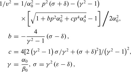
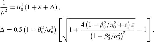
where ν is the phase velocity, p is the ray parameter (projection of the slowness vector onto the bedding plane) and α₀, β₀, ɛ and δ are Thomsen anisotropy parameters. The parameters are the P- and S-wave velocities along the symmetry axis, ɛ is the P-wave anisotropy parameter and δ is the parameter controlling the deviation of the wave front from an ellipsoidal geometry. Because of the generally small size of the ultrasonic transducers (6mm in diameter) as compared to the propagation path (few centimetres) in the experiments described below, the measured wave velocities are likely to be ray (group) velocities (Dellinger & Vernik 1994; Vestrum 1994; Dewhurst & Siggins 2006). The magnitudes of the ray and phase velocities are related through

2

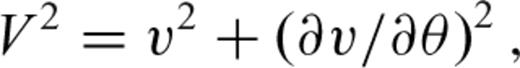
where V is the P-wave ray velocity and is the phase angle. The derivative can be expressed as a function of the ray parameter p,

3

and the derivative can be computed using eq. (1). Therefore, the ray velocity V can directly be expressed as a function of the ray parameter p.

To make use of this relationship, the spatial orientation of the bedding plane, which defines the ray parameter, needs to be known, as p is the projection of the phase slowness onto the bedding plane. In other words, for a cylindrical shale sample that is not cored in a direction normal to the bedding plane, computing the ray velocity for rays propagating off the bedding plane is not straightforward, as the effect of the tilting of the symmetry axis with respect to the sample axis needs to be accounted for, as illustrated in Fig. 1. In this figure, all the ray , slowness and symmetry axis vectors are in the same plane. For a given ray path, the ray angle can be written as a function of the other geometrical parameters as

4

where is the ray angle defined from the symmetry axis ; is the ray incidence angle defined from the vertical or sample axis (z-coordinate); and (which is equal to ) are the dip and azimuth angles of the symmetry axis and is the azimuth angle of the ray vector (see Appendix). Alternatively, the ray angle can be written in terms of the ray parameter (Ursin & Stovas 2006)

5

Figure 1

Schematic illustration of the arrangement of the ray and slowness vectors with respect to the symmetry axis in the tilted transversely isotropic configuration: is the projection of slowness vector onto the isotropy (bedding) plane; and the z-coordinate axis corresponds to the axis of the cylindrical shale sample (modified from Tsvankin 1997).

Open in new tabDownload slide

Using eq. (5) for a given transversely isotropic medium (given Thomsen parameters and orientation of the symmetry axis) and a given ray angle, it is possible to estimate the corresponding ray parameter p through an optimization method described in the next section.

For the rays propagating in the bedding plane, computing the ray parameter is trivial, because the ray parameter is simply the inverse of the phase velocity. To avoid numerical instabilities that may arise from this special case, we check whether the ray vector is parallel to the symmetry axis by computing the scalar product of and ,

6

7

8

where and are unit vectors parallel to the ray and the symmetry axes, respectively. If eq. (8) is satisfied, no optimization is performed. This situation is still used for the estimation of the anisotropy parameter ɛ and the orientation of the symmetry axis.

Computation of the Ray Parameter

In principle, it is possible to estimate the ray parameter p for a given transversely isotropic medium and a given ray angle using directly eq. (5). However, to avoid numerical instabilities associated with the square root of negative numbers, it is more convenient to rewrite it in the form

9

where f = 0. This equation has only one root for the above conditions and this root can be numerically determined using the Newton–Raphson method for instance (Press et al. 2007). This algorithm converges quickly in most cases where the anisotropy parameters are within realistic values and for rays propagating in directions not too close to the bedding plane. For odd values of the anisotropy parameters and when the ray propagates in directions subparallel to the bedding plane, it is more difficult to bracket eq. (9), which means that the algorithm converges more slowly and not always to the root value. In such situations, an alternative method is preferred. It consists of the use of an optimization algorithm to minimize, with respect to the ray parameter p, an objective function that quantifies the difference between a ‘measured’ and a computed ray angle,

10

where the subscripts m and c stand for the ‘measured’ and computed ray angles using eqs (4) and (5), respectively. Newton's algorithm is employed to minimize the above objective function.

For both methods, a random ray parameter is drawn from a uniform distribution to start with. For this selection, the lower bound is set to zero and the upper bound is set to the inverse of the slowness vector (Thomsen 1986),

11

In extremely rare situations, when the ray propagation direction is very close to the symmetry plane, the objective function (10) may lose its convexity. This typically slows down the convergence although the algorithm takes further iterations.

Estimation of the Anisotropy Parameters and the Symmetry Axis Orientation

To determine the spatial orientation of the symmetry axis (ϕ,ω) and anisotropy parameters, , an objective function is defined (Tarantola 2005) with the P-wave ray velocities taken from eq. (2). This function is minimized using the VFSR (Ingber 1989),

12

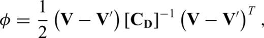
where V are the measured ray velocities (from all the selected source–receiver pairs), are the synthetic ray velocities associated with a given set of model parameters (for the same set of source–receiver pairs) and the superscript T stands for the transpose operator. [ C_D ]⁻¹ is the inverse of the covariance matrix of the errors in the ray velocity measurements. The diagonal elements of C_D are variances and are identical for all the measurements. Assuming there is no correlation between the residual errors of the ray velocities, the off-diagonal elements (covariances) of the matrix C_D are null. Where required, an additional minimization process is applied following the convergence of the VFSR algorithm, to achieve a convergence to the true solution. For this additional step, a non-linear conjugate gradient algorithm is used (Nocedal & Wright 1999; Press et al. 2007). Both minimization algorithms require the derivatives of the objective function with respect to the model parameters, namely,

13

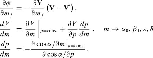
The derivatives of the ray velocity with respect to the model parameters and the ray parameter are available in eqs (1)–(3). The azimuth angle is related to the model parameters and to the ray parameter p through the ray angle in eq. (5). The derivatives of the ray velocity with respect to the coordinates of the symmetry axis are,

14

15

where , and can be computed from eqs (4) and (5). For a ray propagating within the bedding plane, the derivatives of the ray velocity V with respect to the anisotropy parameters can be obtained directly from eq. (11). Note that in this particular propagations direction, dV/dδ, dV/dϕ and dV/dω are null. To estimate the anisotropy parameters and the orientation of the symmetry axis, a prior set of values is randomly drawn from a uniform distribution constrained to the lower and upper bounds given in Table 1. To prevent the algorithms from converging towards an undesired set of model parameters, the following additional constraints are imposed on the sampling. In particular, the sampling of the anisotropy parameter should be given special attention such that it should never produce a negative elasticity stiffness C₁₃. In fact, a heuristic approach is employed to constrain C₁₃ (and ) to avoid any numerical instability in particular for the computation of the ray parameter,

Table 1

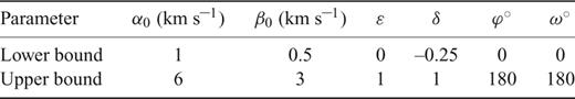
Lower and upper bounds imposed on model parameters during the minimization procedure.

Open in new tabDownload slide

The VFSR is run for example up to 5000 iterations (annealing temperature) with 100 model selections at each temperature, then the best jump is chosen by scanning the objective function at each iteration to find the minimum. The decay factor and initial temperature during the VFSR for all the model parameters are similar, that is 0.9 and 1000, respectively. As discussed thoroughly in Tsvankin (2001), in a transverse isotropic medium has negligible effect on the P-wave phase velocity even for uncommonly strong velocity anisotropy. In the context of the inverse problem, this small sensitivity would not be enough to have a reliable estimate of from actual experimental data. However, in a noise-free numerical example as discussed by Nadri et al. (2011b), it is possible to estimate using a gradient search method such as the conjugate gradient with a prior model close to solution. Within the limit of the weak anisotropy (), linearized P-wave phase velocity equation (Thomsen 1986) does not depend on the .

Application of the Method To Laboratory Data

As the first validation example, P-wave ray velocity measurements obtained on a spherical shale sample (Fig. 2) are used. The ultrasonic array consists of 132 source–receiver pairs evenly distributed over the entire sphere (Bóna et al. 2012). This argillaceous siltstone is of late Jurassic to early Cretaceous age and is fairly homogenous. As reported by Bóna et al. (2012), the original core sample was polished in different directions to form a sphere with 50 ± 0.01mm diameter. The sample was then covered with a thin layer of epoxy resin and placed in an oil-filled pressure vessel at ambient temperature and 40 MPa confining pressure. Source and receiver piezoceramic transducers were identical with a diameter of 5mm and a resonant frequency of 2 MHz. P-wave velocity measurements across the sphere are performed every 15° in the azimuthal and polar directions; for each measurement the source and the receiver face each other, at opposite ends of a diameter of the spherical sample (see Bóna et al. 2012). A comprehensive description of the experimental set-up is given by Pros et al. (1998). Table 2 shows a comparison between the estimates obtained with the current approach (‘coupled inversion’) and the previous approach described by Nadri et al. 2011a (‘uncoupled inversion’). The two estimates are very similar. Note that the results for are not displayed for the reasons given in the previous section.

Figure 2

A spherical shale sample from the North West Shelf in Western Australia.

Open in new tabDownload slide

Table 2

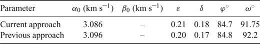
Comparison of Thomsen anisotropy parameters and symmetry axis orientation as estimated with the current approach (‘coupled inversion’) and with the earlier approach (‘uncoupled inversion’).

Open in new tabDownload slide

The ‘uncoupled inversion’ had some drawbacks that are overcome in the new ‘coupled inversion’. For instance, numerical derivates were used to compute the phase angle, although analytical expressions of the derivatives are now used. Also the data had to be linearly interpolated with respect to the azimuth and polar angles to improve the accuracy of the numerical derivatives. Such interpolations are no longer required in the current ‘coupled inversion’. Although the overall computation time is similar in both approaches, the ‘uncoupled inversion’ required more effort for manual data preparation and analysis to find the symmetry axis coordinates.

As a second example of application of the ‘coupled inversion’ we use the P-wave ray velocities measured on a cylindrical shale sample (Fig. 3) subjected to 45 MPa confining pressure and 5 MPa pore pressure in an Autonomous Triaxial Cell (ATC). This apparatus allows for the application of axisymmetric triaxial stresses (σ₁≠σ₂ =σ₃) using hydraulic oil as the confining medium and a hydraulic actuator to apply the axial stress. The data acquisition system consists of a multichannel ultrasonic monitoring apparatus directly attached to the ATC. An array of 16 miniature ultrasonic P wave transducers (6mm in diameter, 500 kHz resonant frequency) is directly attached to the lateral surface of the cylindrical shale sample through a Viton sleeve (Fig. 4). This sleeve aims at (i) isolating the specimen from the confining medium (hydraulic oil) and (ii) control the pore fluid pressure independently from the applied confining pressure. A comprehensive description of the experimental set-up is given by Sarout et al. (2010).

Figure 3

A cylindrical shale sample from the Opalinus Clay formation in Switzerland. The grey lines indicate the apparent orientation of the shale bedding plane.

Open in new tabDownload slide

Figure 4

Spatial arrangement of the array of P wave ultrasonic transducers attached directly to the lateral surface of the shale sample through a Viton sleeve.

Open in new tabDownload slide

A velocity survey is performed on the cylindrical shale sample: each of the 16 transducer acts sequentially as a source although the other transducers record the transmitted pulse on the same time basis. Of all possible source–receiver combinations, 204 direct arrival traveltimes are picked. Source–receiver combinations leading to ray paths propagating near the surface of the sample are not used. Some of the 204 measurements are recorded from reciprocal shots on a given pair of transducers; these repetitive measurements are averaged. To check the accuracy of the parameter estimation, we have estimated the model parameters using the noise-free synthetic data for the above cylinder with the same acquisition configuration (Nadri et al. 2011b). Although the VFSR recovered all the parameters except accurately, a conjugate gradient method applied afterward recovered all the parameters including . The VFSR does not always sample at the exact location of the minimum but rather around it, whereas gradient methods, such as the conjugate gradient converge to the exact minimum. In this context, where only P-wave velocities are available, is in a relatively flat area in the objective function. Hence, only in a noise-free system can it be estimated using for example a gradient minimization method.

The ray path lengths are then required to compute the P-wave ray velocities. The correct source–receiver ray path length is a challenging issue in ultrasonic measurements, in particular for source–receiver pairs not located directly opposite each other. The minimum distance between finite-sized transducers is not a good proxy for the actual distance energy travel. To address this issue, a velocity survey using the same array of transducers is performed on a cylinder made of isotropic Lucite with a size identical to that of the shale sample. The uncertainty in the spatial positioning of the ultrasonic transducers is of the order of 1mm. This calibration survey is used to determine the effective propagation length for each source–receiver pair since the P-wave velocity in Lucite is known. These effective propagation lengths are then used to compute the ray velocities for the actual shale sample. The estimated parameters for the best solution from the VFSR are shown in Table 3. This indicates that the symmetry axis for this shale sample is tilted with an angle of 30° with respect to the axis of the cylindrical sample, which is qualitatively consistent with the bedding plane orientation obtained by visual inspection of the lateral surface of the sample (see Fig. 3).

Table 3

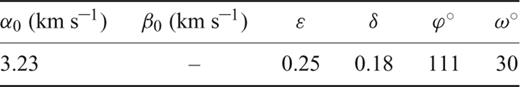
Estimated Thomsen anisotropy parameters and symmetry axis orientation estimated with the current approach (‘coupled inversion’) for the cylindrical shale sample.

Open in new tabDownload slide

Summary and Conclusions

A new method for simultaneously estimating Thomsen anisotropy parameters and the orientation of the symmetry axis for transversely isotropic rocks from laboratory P wave ultrasonic data is reported (‘coupled inversion’). This method has been validated against an earlier technique (‘uncoupled inversion’). Both methods are useful when the orientation of the symmetry plane or axis are unknown in transversely isotropic rocks such as shales. However, although the ‘uncoupled inversion’ method is hard to implement for geometrical shapes other than the spherical samples configuration (transducers facing each other) because of insufficient measurements along the polar and azimuthal directions to compute the spatial derivatives of the ray velocity, the new ‘coupled inversion’ technique can be used for any source–receiver configuration (any array of source–receiver arranged in a ‘tomography’-like configuration). It has been applied to a cylindrical shale sample in the laboratory and the estimated orientation of the symmetry axis appears to be qualitatively in agreement with the visual inspection of the sample.

The new method of geometry-independent, coupled inversion of P-wave ray velocity data to determine the magnitude and orientation of transverse isotropy in rocks, relies on the computation of the ray parameter and is extremely fast, in particular using the root-finding approach. We used VFSR to minimize the objective function of the ray velocity residuals, which guarantees convergence to the optimum solution. Note that no assumption is made regarding the magnitude of anisotropy (no weak anisotropy assumption), neither in the ray parameter computation nor in the minimization procedure. It has also been checked that the ‘coupled inversion’ does not fail in the case of strong anisotropy. Despite the stochastic nature of the VFSR, requiring up to a million evaluations of the objective function, the minimization procedure takes less than 5 min on a Quad core Intel processor X5570 series using a serial programming C++ code.

Acknowledgments

We would like to thank the Editor, Professor Jeannot Trampert and two reviewers, Professor Yves Guéguen and Dr. Tatiana Chichinina for their invaluable comments and suggestions which improved the quality of the manuscript.

References

Appendix

Fig. 1 shows the ray propagation vector and symmetry axis vector in a transversely isotropic medium. We can express these vectors in terms of the unit vectors and are given in expressions A1 and A2, respectively. Using the scalar product of the ray and symmetry axis vectors, we can express the ray angle in terms of other geometrical angles which is given in A3. is the ray angle of incidence, is the ray angle, is the tilt angle of the symmetry axis, is the azimuth of the ray vector and is the azimuth of the symmetry axis.

(A1)

(A2)

(A3)