Subevent location and rupture imaging using iterative backprojection for the 2011 Tohoku M_w 9.0 earthquake

Summary

1 Introduction

An important seismic problem is understanding the rupture processes of large earthquakes. Conventional (time-domain) backprojection of teleseismic P waves, starting with Ishii et al. (2005), is a popular and efficient method to determine the rupture extent, duration and speed of large earthquakes (Walker et al. 2005; Ishii et al. 2007; Walker & Shearer 2009; Xu et al. 2009; D'Amico et al. 2010; Kiser & Ishii 2011; Zhang & Ge 2010). Backprojection methods are similar to migration techniques in reflection seismology in that they use simple ray theory to compute time-shifts for stacking seismograms at candidate source locations. They are related to time-reversal (or reverse-time) imaging of sources or reflectors (e.g. Fink 1992; Ekström et al. 2003; Larmat et al. 2006), but are faster to compute because they do not need to solve for the complete Green's functions for the seismograms. Instead, the backprojection approach approximates the Green's function simply as a time delay that does not change the amplitude or shape of the waveforms. As such, backprojection works best for uncomplicated portions of body-wave traveltime curves that do not suffer from triplications, large amplitude changes or significant dispersion. Fortunately, mantle P waves at epicentral distances between 30° and 95° meet these criteria and include a large fraction of observed seismograms. Empirical corrections for the small time-shifts caused by 3-D mantle structure along the source-to-receiver ray paths can be obtained using waveform cross-correlation on the first arriving waveforms, which originate from the hypocentre (Ishii et al. 2005). These advantages make backprojection a valuable near-real-time technique to analyse large earthquake rupture processes. Backprojection provides information on high-frequency radiation, which is a useful complement to other approaches to study earthquakes, for example, seismic slip inversions (Ji et al. 2002; Uchide & Ide 2007), which use local or teleseismic low-frequency waveforms to invert for the detailed slip distribution, rupture speed and moment rate functions at one or multiple fault planes.

The resolution of the conventional backprojection method is limited by the frequency range of the data and the array geometry used. Low-frequency P waveforms (f < 0.1 Hz) are less affected by scattering and small-scale heterogeneity and therefore are easy to stack coherently. However, their relatively long wavelengths result in poor lateral resolution for backprojection source imaging. On the other hand, high-frequency data (f > 1 Hz) should be able to achieve good resolution considering their short wavelengths, but their waveforms are more easily distorted by small-scale heterogeneity and scattering, which results in less coherent waveform stacks and poorer source imaging. So far, the most successful frequency band for backprojection studies using teleseismic P waves is 0.2–1 Hz (e.g. Ishii et al. 2005; Walker & Shearer 2009; Xu et al. 2009). In this band the lateral resolution and waveform coherence are well balanced to produce optimal source images. Array geometry is another important factor that controls the lateral resolution of backprojection images. In theory, global stations should give better resolution due to their superior azimuthal coverage. However, in practice regional arrays seem to work better. This is probably because waveforms from regional arrays are less affected by 3-D heterogeneity, waveform complexities (e.g. depth phases), and source effects (e.g. due to focal mechanism) and therefore more coherent for stacking than the more distributed global stations. Results from a single regional array sometimes show smearing of source images in certain directions, which depends on the geometry of the array (Ishii et al. 2005; Xu et al. 2009). Thus, combining different regional arrays can often achieve better resolution and less smearing of the source images (Xu et al. 2009; Kiser & Ishii 2011). The depth resolution of backprojection images using only the teleseismic P phase is very poor due to nearly vertical take-off rays in the source region (Xu et al. 2009). However, Kiser et al. (2011) recently showed that combining depth phases (i.e. pP or sP) with the direct P phase in the backprojection method can provide good depth resolution for deep sources in which the depth phases are visible.

Although backprojection has been successful in imaging the gross rupture properties of big earthquakes, its ability to resolve small-scale details of the rupture process is limited by the relatively coarse resolution of the backprojection operator, the rapid oscillations in the raw backprojection time-series and the presence of ‘sweeping’ artefacts in backprojection images, which propagate towards the stations at high speed (i.e. the P-wave phase velocity at the recording stations). The conventional backprojection method first obtains the waveform stack, which is a time-series, at each grid location in the source region. To obtain stable estimates of energy radiation, the raw waveform stack is averaged over a smoothing interval that reduces the temporal resolution but removes some image artefacts. The duration of this time window is typically about 10–30 s (Ishii et al. 2005; Xu et al. 2009) and sometimes both space and time averaging are performed to suppress the ‘sweeping’ artefacts (Walker & Shearer 2009). Rupture velocity is then typically estimated by selecting locations and times of peak energy radiation along the fault (e.g. Ishii et al. 2005). However, this time averaging may limit the subevent details that can be resolved, such as their number, duration, location and time.

Our approach here is to consider more explicitly the possibility that the rupture can be modelled as a series of subevents (large energy bursts), rather than a smooth continuous rupture. Our method applies a waveform cross-correlation and signal stripping technique to iteratively identify subevents from the backprojection results. The time-shifts from the waveform cross-correlation can then be used to locate the subevents more precisely than can be obtained from the backprojection images. Once a subevent is found, its principal waveforms are determined from principal component analysis and then subtracted from the seismograms. The residual seismograms are then used to identify the next largest subevent. In this way, the waveforms are modelled as a series of subevents (defined by their times, locations and amplitudes), which can be used to characterize the rupture properties and dynamics of the earthquake.

The idea of decomposing a big earthquake into a number of subevents has a long history in seismology. For example, Wyss & Brune (1967) used six subevents to explain the pulses in teleseismic P records of the 1964 Alaska earthquake. Recently, Tsai et al. (2005) applied an iterative multiple-source centroid-moment-tensor (CMT) analysis (inversion) to the 2004 Sumatra earthquake and identified five subevents to fit the long-period waveforms. Our time-domain signal stripping technique shares some similar features to the mode-branch stripping technique for measuring surface wave overtone phase velocities (Van Heijst & Woodhouse 1997). It is also analogous to the CLEAN algorithm used in the frequency domain in radio astronomy (Högbom 1974) and for multimode surface wave dispersion analysis (Nolet & Panza 1975).

Because our method is largely empirical, it is difficult to address questions of uniqueness and resolution in our results formally. As a substitute, we perform both bootstrap resampling tests of our data and synthetic tests to evaluate how well we can recover various scenarios of subevent distributions and time histories. Ideally, with good data coverage in azimuth and distance, our method works if the subevents are separated in either space and time. However, in practice using a regional array with a limited aperture, our method works best when the subevent waveforms are well separated in time, in which case in principle we obtain better time and space resolution than conventional backprojection. Our method has trouble when the subevent waveforms overlap substantially in time at most stations. In this case, other methods, such as the frequency-domain approach of MUSIC (Schmidt 1986; Meng et al. 2011) and compressive sensing (Yao et al. 2011) work better in simultaneously resolving multiple subevents, but at the cost of poorer time resolution than our signal stripping approach.

To illustrate the method, we use teleseismic P-wave data recorded in the United States from the 2011 Tohoku M_w 9.0 earthquake in Japan. In Section 2, we provide the basic theory and mathematical formulation of the backprojection method for a large earthquake consisting of multiple subevents. The conventional backprojection method and the proposed iterative backprojection method are illustrated in Sections 3 and 4, respectively. Section 5 gives a method to relocate the subevents obtained from iterative backprojection. Section 6 shows the results of the spatial and temporal distribution of subevents of the Tohoku earthquake, which are used to estimate the rupture speed of this earthquake. In Section 7 we show some results of synthetic tests, the effects on subevents from depth phases, the reliability of the identified subevents from bootstrap approaches and compare our results with other backprojection results and slip inversion results.

2 Basic Theory of Backprojection

During the rupture of a large earthquake, seismic energy is radiated from the source region and recorded by seismometers around the globe. If we treat large energy bursts as subevents during the main shock, the record at each station can be viewed as a sum of waveforms generated by subevents. The received signal V_i(t) (usually a velocity seismogram) at the ith station due to N_s subevents can be modelled as

1

where t is the recording time, a_k(t) is the kth subevent source time function, G(x_k, x_i, t) is the Green's function from the source location x_k to the receiver location x_i and n_i(t) represents random noise. To determine the subevents, we assume that the Green's functions are mainly due to one wave type (e.g. direct P waves), therefore,

2

where G_ik is the amplitude of the dominant wave type, t_ik = t(x_k, x_i) gives its traveltime from x_k to x_i, and g(x_k, x_i, t) is the Green's function of other minor phases (including scattering) with amplitude much smaller than G_ik. Eq. (1) is then modified to

3

where is called the residual waveform.

We assume that all subevents are close enough relative to the propagation distance (e.g. at teleseismic distances) so the amplitudes of the subevent Green's function may be approximated as constant (G_ik = G_i) and therefore

4

We assume that each subevent has starting time t^(k), duration δt^(k) and amplitude C_k,

5

where is a normalized time history (). Hence, eq. (4) becomes

6

Each trace is then normalized with its maximum amplitude C^max = max{V_i(t)} so that

7

where v_i(t) =V_i(t)/C^max is the normalized waveform, , is the normalized residual waveform that includes waveforms of minor phases and noise and is the normalized kth subevent waveform.

The backprojection image is simply a slant stack of traces along some traveltime curve, which approximates the source time history at each model point as the weighted sum of the data points it affects. In a general case with consideration of other minor phases and noise (eq. 7), the source time history at grid location x_m is approximated by backprojection (slant stack) of all N normalized seismograms:

8

where t gives the source time. When the potential source location x_m is at a subevent location x_k, that is, t_im = t_ik, the waveforms due to the dominant phase will stack coherently only at the source location x_k (first term in eq. 8) and the other minor phases (with different traveltime moveout) and noise (second term in eq. 8) will stack incoherently, so

9

approximates the source time history at source location x_k. These methods thus allow for investigation of multiple subevents in both space and time from backprojection.

3 Conventional Backprojection

In this section, we demonstrate the conventional backprojection method using the first 170 s of vertical component waveforms of the M_w 9.0 Tohoku earthquake, which contain mainly teleseismic P-wave data, as recorded by about 500 stations in the western and central United States (including 370 USArray stations). The stations are at distances of 65°–94° from the epicentre. Waveform data are first filtered to a relatively broad band (0.05–4 Hz) and the amplitude of each trace is normalized to unit peak.

To obtain the coherent stack at the subevent location (eq. 8), we need to know the traveltime t_ik from the source location x_k to each receiver at x_i. The traveltimes are obtained from a 1-D Earth model, with empirical corrections for 3-D structure computed from waveform cross-correlation of the initial part of the P wave. The waveforms are first aligned after correcting for the predicted P-wave propagation time from the hypocentre location [lat 38.19°, lon 142.68°, depth 21 km; from Chu et al. (2011)] to the station using the IASP91 1-D earth reference model (Kennett & Engdahl 1991). However, due to 3-D heterogeneity of the Earth structure, the P waves are not perfectly aligned, and additional time corrections must be applied to ensure a coherent stack. This is usually achieved by cross-correlating the first few seconds of the P waves to determine the additional time-shifts for each seismogram. Here we apply a multichannel cross-correlation method (VanDecar & Crosson 1990) and clustering analysis (Romsburg 1984) for the first 8 s of the P waves. Seismograms from the largest cluster and with correlation coefficient above 0.6 are linearly stacked to generate a reference stack (the black trace in Fig. 2). The reference stack is then correlated against each seismogram (still for the first 8 s of the P waves) to obtain the correlation coefficient and polarity with respect to the reference stack. Then seismograms with correlation coefficients above 0.6 and positive polarity are stacked to generate the next-generation reference stack (Ishii et al. 2007). The process is repeated a few times to obtain the stable additional time-shifts and polarity information (p_i =±1, due to focal mechanism) with respect to the reference stack for each seismogram. For all subsequent analysis we use only data from stations that have initial P waves with positive polarity (relative to the reference stack). The distribution of stations is shown in Fig. 1. The selected trace is then 0.2–1 Hz bandpass filtered and normalized, denoted as v_i(t) at the ith station (i = 1,…, N = 476).

Figure 2

(a) Top panel: first 170 s of the vertical-component waveform (0.2–1 Hz bandpass-filtered and normalized) recorded by stations in the western and central United States (Fig. 1). Bottom panel: the stack s(x, y, t) (eq. 11, black) of all the traces and the time-averaged stack power P(x, y, t) (eq. 12, red) at the hypocentre (x, y) = (0, 0). The two vertical lines indicate the first 8 s of the P-wave window for the initial waveform cross-correlation and alignment using a broader frequency band (0.05–4 Hz). The traces are sorted in an azimuth-ascending order. (b) First 15 s of the P-wave window after alignment.

Open in new tabDownload slide

Figure 1

Epicentre of the 2011 Tohoku earthquake (red star) and the stations (blue triangles) in the western and central United States used for the iterative backprojection.

Open in new tabDownload slide

The final aligned P waveforms u_i(t) (Fig. 2) with respect to the hypocentre event are defined as

10

where t is the source time.

The traveltime perturbation accounts for the heterogeneity along the ray path from the hypocentre to the station. If we assume the source region (earthquake rupture area) is small compared to the epicentral distances and its structural variation is not large, should also approximate the traveltime shift with respect to the 1-D reference model from other grid locations in the source region to the station due to very similar paths. Therefore, the traveltime from each source location x to station at x_i is given by , where is the reference traveltime from x to x_i using the 1-D reference model.

For conventional backprojection using a linear stack, the seismograms are summed to make the stack s(x, t) as a function of the source time t and the source location x = (x, y, z):

11

where p_i and w_i are the polarity and amplitude weight of the ith seismogram, and . The amplitude weights are normalized such as . The weight w_i can be determined using a station-weighting scheme from the spatial density of stations (Walker et al. 2005; Walker & Shearer 2009). In this study we simply set w_i = 1/N considering the relatively even distribution of the array stations. Here we define the hypocentre location at x = (x, y, z) = (0, 0, H), where H = 21 km is the focal depth. For this study the coordinates of all other locations in the source region for backprojection are with respect to the hypocentre location, with x and y being positive to the east and north of the hypocentre. For teleseismic waveform backprojection only using P waves, the depth resolution is poor (Xu et al. 2009), thus we only backproject waveforms on the 2-D plane at the focal depth. From here on, we drop z in all expressions for simplicity.

Since s(x, y, t) is a stacked waveform, it cannot be directly used to represent the source power. We often compute a running-window time-averaging of s²(x, y, t) to obtain the time-averaged stack (or source) power P(x, y, t) and amplitude A(x, y, t) as

12

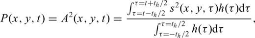
where h(t) is the window function and t_h gives the window duration. Typically h(t) is set to a boxcar function (Ishii et al. 2005), that is, h(t) = 1 for t∈ [−t_h/2,t_h/2], and therefore P(x, y, t) is the mean squared amplitude of the windowed stack waveform. In this study we set h(t) as the Hann window (symmetric cosine taper function) with for t∈ [−t_h/2,t_h/2]. The use of the Hann window instead of the boxcar window may suppress some edge effects of time averaging. An example of the stacked waveform and the stack power (with t_h = 10 s) is shown in Fig. 2(a).

The time-integrated stack power and amplitude from the backprojection is defined as

13

where t_s and t_e are the starting and ending source times for backprojection.

It is possible that strong 3-D local heterogeneities exist within the source region. Therefore, for subevents that are far away from the hypocentre, the traveltime perturbations due to regional 3-D structural heterogeneities are different from in eq. (10). This may result in less coherent stacks of the waveforms at some imaging locations. Ishii et al. (2007) introduced a time calibration method using aftershocks to account for this effect, but found that the changes were relatively small for the backprojection image of the 2004 Sumatra earthquake. However, this effect likely causes at least some underestimation of subevent amplitudes due to less coherent waveform stacks at increasing distances from the hypocentre.

For the backprojection waveform stack (eq. 11), we only use waveforms which have correlation coefficients above 0.6 and positive polarity with respect to the reference stack. For those traces with negative polarities and smaller correlation coefficients we can simply set the weight w_i = 0 in eq. (11). The time-integrated stack power of the Tohoku earthquake is around the hypocentral area if we use data filtered between 0.2 and 1 Hz (Fig. 3a). However, the peak stack power shifts about 70 km towards the Japan coast with respect to the hypocentre for high-frequency data (1–2 Hz; Fig. 3b), which suggests frequency-dependent energy radiation of this earthquake (Yao et al. 2011; Koper et al. 2011b).

Figure 3

Time-integrated stack power in the frequency band 0.2–1 Hz (left-hand side) and 1–2 Hz (right-hand side) from conventional backprojection with the epicentre location determined by Chu et al. (2011) and the strike orientation of the Tohoku earthquake from USGS W–Phase moment tensor solution (dashed) (; last accessed on 2012 February 15).

Open in new tabDownload slide

4 Methodology of Iterative Backprojection

In principle we can decompose the original seismograms v_i(t) as the sum of subevent waveforms and residual waveforms (eq. 7). Similarly for the aligned waveforms u_i(t), we decompose it as the sum of waveforms from N_s subevents, , and the residual waveforms as

14

We search for all local maxima of the time-averaged stack amplitude [A(x, y, t) in eq. 12] of the conventional backprojection (eq. 11; see Fig. 4a for an example). A few local maxima will cluster in space and time and tend to have similar arrival times to stations and many of them have small amplitudes. We perform a local maxima declustering process to remove insignificant maxima. First local maxima with amplitude less than 0.05 of the global maximum are removed. Secondly, starting from the largest local maximum, we remove any other smaller local maxima that will arrive at a similar time (within 5 s) with respect to the arrival time of the selected local maximum to a reference station in the centre of the array. This largest local maximum is considered as the ‘significant maximum’ and then removed from the list of the local maxima. This process is repeated for the remaining local maxima until there is only one local maximum left in the list. The obtained significant maxima (location and time) are shown in Fig. 4(b) and will be considered as possible subevents for the iterative backprojection analysis.

Figure 4

(a) Locations and times of all local maxima (coloured circles) and (b) the significant maxima (coloured circles) of the time-averaged stack amplitude A(x, y, t). The subevent waveform amplitude is proportional to the radius of circle. The colour bar shows the source times of maxima. The plus symbol (+) in (b) shows the maximum.

Open in new tabDownload slide

The iterative backprojection approach combines the conventional waveform backprojection method with subevent signal stripping to determine the location, time, duration and waveforms of each individual subevent in an iterative way. At each iteration, parameters for the next subevent (preliminary location and source time) are estimated from the local maxima (Fig. 4b) in the temporally smoothed stacked image. We then window subevent waveforms and re-cross-correlate them with their stack to compute correlation coefficients and additional traveltime shifts. The duration of each subevent is determined by the length over which the signals are well correlated with the stack using a short-time running-window cross-correlation method. Principal component analysis is then used to extract the subevent principal waveforms within the determined time window. The next-generation residual waveform is then obtained by subtracting the subevent principal waveforms from the current residual waveforms, which we term ‘subevent signal stripping’. This process is repeated until no more qualified subevents can be identified from the residual waveforms. After larger subevents have been identified and their waveforms are stripped out, smaller subevents can be identified one after another. The final residual waveforms and the waveforms from each subevent are individually backprojected and summed together to form the final backprojection stack. Using the additional time-shifts derived from the subevent waveform re-cross-correlation, we can locate the subevents more accurately than can be estimated from the conventional backprojection image, which should translate into improved estimates of rupture speed. The flow chart in Fig. 5 shows the steps of this iterative method, which are listed as follows:

Figure 5

Flow chart of the iterative backprojection method.

Open in new tabDownload slide

• 1

  Bandpass-filter and align (using waveform cross-correlation) the seismograms with respect to the initial hypocentre subevent using the first few seconds of the P waves (see Section 3 for the detail).

• 2

  Perform backprojection of the residual waveforms and obtain the stack s(x, y, t) at each grid location in the source region. The residual waveforms are initially the original seismograms u_i(t) (see eq. 10) and k = 1.

• 3

  Determine the preliminary subevent locations and source times. Here we first determine the significant maxima of the time-averaged stack amplitude (Fig. 4b). These maxima are potential subevents to be further analysed. The first subevent is the significant local maximum at the hypocentre (x⁽¹⁾, y⁽¹⁾) = (0, 0) with the source time corresponds to the maximum of the time-averaged stack amplitude A(x, y, t), using the first few seconds of the P waves. This is because the initiating subevent is free of contamination by later subevent waveforms. For later subevents, we choose the location and source time corresponding to the largest significant maximum (e.g. + in Fig. 4b) as the preliminary kth subevent location (x^(k), y^(k)) and source time . Note that if this is not a qualified subevent (see step 5), we choose the next largest significant maximum as the subevent.

• 4

  Obtain the additional traveltime shifts of the selected subevent waveforms by re-cross-correlating the windowed subevent waveforms with their reference stack using the adaptive stacking approach (Rawlinson & Kennett 2004). To achieve subsample accuracy of time-shifts from cross-correlation, we first interpolate the data and the reference stack to 50 Hz sampling rate using cubic spline interpolation. Based on the preliminary source time , we window the waveforms for the ith station in the time window to obtain the dominant subevent waveforms (e.g. within the two vertical lines in Fig. 6a), where Δt_w is the window length. Δt_w is set to 5 s, corresponding to the longest period in the frequency band ([0.2, 1] Hz here). The (windowed) reference stack is cross-correlated against each windowed subevent waveform to obtain the cross-correlation coefficient , polarity and additional time-shifts (Fig. 6b). Seismograms with positive polarities and correlation coefficients above 0.6 are stacked to create the next-generation reference stack. This step is repeated three times to obtain a stable reference stack and traveltime shifts for each trace. If the subevent location is close to the hypocentre, is small, mostly less than 0.5 s for most traces from our experience (see Fig. 6d for an example). Therefore, we set the maximum time-shifts (Δt_max) allowed in the re-cross-correlation to be 1.0 s. Small Δt_max may preclude some possible subevents from being selected, while large Δt_max may produce cycle-skipping problems in the cross-correlation and selection of unqualified subevents (see step 5 and eq. 15).

• 5
  Assess whether the identified subevent is a qualified subevent. Since smaller cross-correlation coefficients () and larger additional traveltime shifts ( of the subevent waveforms are likely to indicate a less reliable subevent, the quality coefficient r^(k) of the selected subevent is empirically defined as

  

  15

  where N^(k) is the number of qualifying traces that have a positive polarity ( =1) and correlation coefficients for the kth subevent, and is the standard deviation of the additional traveltime shifts () of the N^(k) qualifying traces, and the summation index j is only picked from the list of the N^(k) qualifying traces. For the first subevent, N⁽¹⁾ = 451 and the quality coefficient is 1.0. Since Δt_max = 1 s, is 0.92, 0.84 and 0.61 if is 0.1, 0.3 and 0.5 s, respectively. From this definition, the subevent with smaller N^(k) and and larger will naturally have a lower quality coefficient, which is reasonable. The subevent we are using as an example has a quality coefficient of 0.94 with N^(k) = 445 and = 0.1 s. If the quality coefficient of the selected subevent is less than 0.7, this subevent is defined as an unqualified subevent, and we go back to step (3) to choose the next significant local maximum (Fig. 4b). If none of the subevents corresponding to the significant maxima meets the threshold of the quality coefficient (0.7 here), we stop searching for subevents and jump to step (8).
• 6

  Determine the approximate duration of the selected subevent by performing a short-time running-window cross-correlation between each aligned qualifying trace [i.e. , with and ], and their reference stack (black trace in Fig. 7a). The window is centred at time t (for t∈ [t_s+ 0.5Δt_w,t_e− 0.5Δt_w]) with duration of Δt_w (5 s here). For each effective trace, we obtain a time-dependent correlation coefficient function (Fig. 7b), which is then averaged to obtain the mean correlation coefficient (MCC), shown as the black curve in Fig. 7(c) (low-pass filtered below 0.5Hz). We first find the peak MCC within the subevent time window in step (4) (within the two vertical lines in Fig. 7c). Typically the MCC deceases quickly from the peak MCC, implying that the waveforms from other subevents (or noise) dominates when t is away from the selected subevent. However, in some cases, the MCC curve may become flat or decrease very slowly, which probably indicates other subevents occurred at a nearby time and location. For determining the approximate duration of the subevent, we choose the time duration that corresponds to the MCC larger than 0.75 times the peak MCC value (red dashed line in Fig. 7c) within the time window bounded by the two most nearby local MCC minima. This approximates the duration of this subevent (with starting time τ_s and ending time τ_e), over which the signals are well correlated with the reference stack. A window function W(t), shown as the green curve in Fig. 7, is set to window the subevent waveforms. W(t) is 1 for t∈ [τ_s,τ_e] and has a cosine taper at each side with a time duration of 0.1Δt_w.

• 7

  Extract the subevent principal waveforms using principal component analysis for the windowed subevent waveforms (only for t∈ [τ_s− 0.1Δt_w,τ_e+ 0.1Δt_w], where W(t) is non-zero). We then subtract the principal waveforms from the current residual waveforms to obtain the next-generation residual waveforms. This step is termed ‘subevent signal stripping’. The windowed subevent waveform (Fig. 8b) can be expressed by an N×M data matrix , with N number of traces and M number of points in each windowed trace (M < N here). can be decomposed using singular value decomposition (SVD) as F = UΛV^T, where is a N×N matrix, is a N×M diagonal matrix with non-negative decreasing real numbers {λ₁,…, λ_M} on the diagonal, is a M×M matrix and ^T denotes the transpose. The principal signal matrix is given by F_P = UΛ_PV^T, where Λ_P is a N×M diagonal matrix with a few of the largest diagonal components {λ₁,…, λ_L} (L≪M) of . If we only keep the signals corresponding to the largest component, the extracted principal signal of each trace is very similar to that of the reference stack. However, the subevent waveforms recorded at different stations may be more complicated than the reference stack due to source complexities, propagation effects and site effects. Therefore, we keep a few of the largest diagonal components (Fig. 8c). We require λ_L > 0.25λ₁. Therefore, less coherent signals or noises associated with smaller diagonal components of are removed. The subevent principal waveform of each trace is obtained from each row of the principal signal matrix F_P. The next-generation residual waveforms (Fig. 8d) are updated by subtracting the subevent principal waveforms (Fig. 8c) from the current residual waveforms (Fig. 8a). Then we reiterate from step (2) for finding the next subevent and k = k+ 1.

• 8
  Perform the backprojection for the final residual waveforms and each subevent principal waveforms after N_s subevents have been identified. The final residual waveform stack S^R(x, y, t) is obtained using eq. (11). We use the additional time-shifts from waveform re-cross-correlation (step 4) to obtain each subevent waveform stack S^(k)(x, y, t) as

  

  16

  We set for non-qualifying traces (with negative polarity () and correlation coefficient ) and for the N^(k) qualifying traces. The complete iterative backprojection stack S(x, y, t) is thus obtained by summing the final residual waveform stack S^R(x, y, t) and all the subevent principal waveform stacks S^(k)(x, y, t), that is,

  

  17

Figure 6

Subevent waveform alignment. (a) Initial 5-s-long windowed subevent waveforms (background image, within the two vertical black lines) and their stack (solid). The subevent time is 88.3 s and the location is (x, y) = (− 30, 20), as shown in Fig. 4(b) (blue +). (b) Cross-correlation coefficients (background image) between the time-shifted subevent waveform and the stack [within the black lines in (a)]. The maximum absolute correlation coefficient is shown by the magenta (positive polarity) or yellow (negative polarity) dot. The colour bar gives the correlation coefficient (b or d) or the amplitude of each (normalized) trace (a or c). (c–d): similar as (a–b), but after three iterations.

Open in new tabDownload slide

Figure 7

(a) Aligned waveforms (background image) and their stack (black trace) for the identified subevent. (b) Short-time running-window correlation coefficients (background image) between each trace and the stack (see text for the detail). (c) Mean correlation coefficient after 0.5 Hz low-pass filtering below (black curve) and the subevent time window (green curve). The red dashed line has a correlation coefficient equal to 0.75 times the peak correlation coefficient within the initial subevent time window (between the vertical black lines).

Open in new tabDownload slide

Figure 8

(a) Aligned current residual waveforms for the identified subevent. (b) Windowed subevent waveforms (between the dashed lines). The window function is shown as the green curve, same as the window function in Fig. 7 (the green curve). (c) The subevent principal waveforms obtained from principal component analysis. (d) The next-generation residual waveforms obtained by subtracting the subevent principal waveforms in (c) from the current residual waveforms in (a).

Open in new tabDownload slide

Fig. 9(a) shows an example of the stack peak amplitude (A_p(x, y) = max{|A(x, y, t)|} for t∈ [t_s,t_e]) from the current residual waveforms (Fig. 8a). The stack peak amplitude using the determined current subevent waveforms (Fig. 8c) is shown as Fig. 9(b). After the waveforms of this subevent are stripped out, the stack peak amplitude of the next-generation residual waveforms (Fig. 8d) is shown as Fig. 9(c), where the next largest subevent (green × in Fig. 9c) appears more visible.

Figure 9

Stack peak amplitude A_p(x, y) = max{|A(x, y, t)|} for t∈ [t_s,t_e] of (a) the current residual waveforms, (b) current subevent waveforms and (c) the next-generation residual waveforms with the locations of the current (blue +) and next subevents (green ×).

Open in new tabDownload slide

Here we define the residual waveform energy ratio as

18

Fig. 10(a) shows the evolution of the residual waveform energy ratio versus number of identified subevents. After 16 subevents (with quality coefficients above 0.7) are identified, the residual waveform energy ratio decreases to 0.25, implying that the 16 subevents contribute 75 per cent of the energy in the waveforms. The final residual waveforms are shown in Fig. 10(b).

Figure 10

(a) Residual waveform energy ratio after each subevent waveforms have been stripped. (b) The final residual waveforms after 16 subevent waveforms have been stripped.

Open in new tabDownload slide

5 Relocation of Subevents

The preliminary subevent locations are determined at the pre-defined (coarse) grid locations corresponding to some significant maxima of the time-average stack amplitude (see the step 3 in Section 4). However, the subevent can be relocated using the relative traveltime shifts () for each subevent determined from subevent waveform re-cross-correlation. Here we use a grid search and ℓ₁-norm method (Shearer 1997) to improve the subevent locations and source times. Due to the poor depth resolution of teleseismic data, we only solve for horizontal locations at the plane of the hypocentre depth, just as for the backprojection imaging.

The predicted traveltime from a location (x, y) to a station using the 1-D model is . For the subevent at the location (x^(k), y^(k)) with the source time , the measured relative traveltime shifts (or traveltime residuals) are , where is the actual traveltime through the real heterogenous Earth. If the source is moved from (x^(k), y^(k)) to (x, y), the traveltime shifts becomes

19

Our goal is finding location (x, y) and a source time perturbation δT_s such that the ℓ₁-norm traveltime misfit function

20

is minimized. Since the source time perturbation δT_s simply gives the baseline shift of the traveltime shifts, we obtain it from the median of the traveltime shifts (Shearer 1997), that is,

21

The use of the ℓ₁-norm (eq. 20) and median (eq. 21) instead of the ℓ₂-norm and mean for source location problems has the advantage of more robust response of the former to outliers in the data (Shearer 1997). 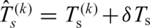We perform the grid search for the subevent relocation on much finer grids (2 km spacing) than the sparser grids used for backprojection (10 km spacing) to find the optimal subevent location and source time perturbation δT_s by minimizing the traveltime misfit function (eq. 20). The new source time at the optimal subevent location is updated by . We show one example of subevent relocation in Fig. 11. The optimal subevent location is about 12 km east and 6 km south of the preliminary subevent location (Fig. 11a) from the iterative backprojection. The traveltime shifts before and after relocation are shown in Figs 11(b) and (c). From the median of the new traveltime shifts after relocation (black line in Fig. 11c), we obtain the source time perturbation δT_s = 0.17 s. Although the traveltime misfit χ decreases as the subevent location moves to the optimal location, some trends in the azimuth-dependent traveltime residuals may remain, which are probably caused by local heterogeneities around the subevent location or contamination by waveforms of other subevents or noise.

Figure 11

Example of subevent relocation. (a) The traveltime misfit χ(s) (eq. 20) distribution with the preliminary subevent location from backprojection (black +) and the optimal subevent location after relocation (yellow +). (b) and (c) show traveltime shifts δt_i(x, y) (eq. 19) before and after subevent relocation, respectively. The black line in (c) gives the median of all traveltime shifts, that is, the source time perturbation δT_s by eq. (21). The trace number is sorted in an azimuth-ascending order.

Open in new tabDownload slide

The location uncertainties using traveltime shifts from waveform cross-correlation can be estimated using a bootstrap approach (Shearer 1997). Here, we randomly select N^(k) traveltime shifts from the total set of N^(k) observed shifts. Then we apply the relocation algorithm described earlier using the N^(k) randomly picked shifts to find the best location. This procedure is repeated 100 times. Finally, the location error is estimated from the standard deviation of the obtained 100 best locations. In the example we show here, the location error is estimated to be about 2.6 km in the E–W direction and 2.0 km in the S–N direction. Since the error of the subevent location is from the formal statistical bootstrap analysis, the true location error is likely larger because we are assuming a simple 1-D model and do not consider effects of contamination from other phases or coherent noise.

6 Results for the Tohoku Earthquake

The iterative backprojection method is used here to image the rupture of the 2011 Tohoku M_w 9.0 earthquake using teleseismic P-wave data (filtered to 0.2–1 Hz; Fig. 2) recorded by the stations in the central and western United States (Fig. 1). Figs 12(a) and (b) show the spatio–temporal distribution of 16 subevents before and after relocation, respectively. The detailed information about the 16 subevents after relocation is shown in Table 1. These 16 subevents are verified as reliable from bootstrap analysis (Section 7.3). The peak of the time-integrated stack power is slightly west of the hypocentre (Fig. 12a). Fig. 13 shows the rupture images (time-averaged stack power of the complete stack S(x, y, t)) at some representative times. The location differences between the subevent locations before and after relocation are shown in Fig. 14(a) and the relocation error is shown in Fig. 14(b), which gives the lower bound of the location error. The time versus distance to hypocentre along the strike of the relocated subevents is shown in Fig. 15.

Figure 12

(a) Normalized time-integrated stack power (red contours) and spatio-temporal distribution of 16 subevents (coloured circles with colour bar showing the subevent time—τ_max in Table 1) from iterative backprojection. (b) Location of 16 subevents (circles) after subevent relocation. (c) Location of aftershocks (M_j > 4, from JMA catalogue; circles) within the first 2 d after the main shock, the relocated subevents (magenta x, subevent time—black number) in the main shock and the dominant slip region [green shaded area (Chu et al. 2011)]. The subevent waveform peak amplitude is proportional to the radius of circle in (a) and (b) and to the size of the magenta x in (c). Each panel shows: epicentre location (black +), the trench location (blue line), the strike (dashed blue) and Japan coastline (black line).

Open in new tabDownload slide

Table 1

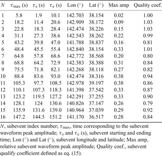
Relocated subevents of the 2011 M_w 9.0 Tohoku earthquake.

Open in new tabDownload slide

Figure 13

Time-averaged power of the complete stack S(x, y, t) at representative times. The colour bar and contours give the normalized power. In each plot: purple star—subevents occurred around the given time with its size proportional to subevent waveform amplitude, blue cross—hypocentre location.

Open in new tabDownload slide

Figure 14

(a) Relative location difference (coloured circles) between new (after relocation) and old locations of all subevents. Positive dx means the new location is more east (closer to the trench) and positive dy more north. The subevent waveform amplitude is proportional to the radius of circle and the colour bar shows the subevent source time. (b) Subevent source location uncertainties in x and y directions from bootstrap analysis of traveltime residuals.

Open in new tabDownload slide

Figure 15

Time versus distance to hypocentre along strike of the subevents. The radius of each circle is proportional to the subevent waveform amplitude and is centred at the time of the maximum amplitude of that subevent. The red bar shows the estimated time duration of each subevent. The numbers in red and black give the time (same as in Fig. 12) and the quality coefficient of the subevent, respectively. Distance is from south to north along the strike (blue dashed line in Fig. 12). Lines of constant rupture velocity are shown in dashed for reference.

Open in new tabDownload slide

From the distribution of subevents (Fig. 12b) this megathrust earthquake shows apparent bilateral rupture features along the strike (N–S) direction and also downdip rupture towards the coast of Japan. The spatial distribution of subevents is more similar to that of the aftershocks (with magnitude above 4.0) within the first 2 d after the main shock than to the major slip distribution inferred from slip inversion (Fig. 12c). Our results show quite complicated rupture behaviour during the first 90 s and dominant high-frequency (0.2–1 Hz) radiation near the hypocentre. In the first 50 s and also at later times (e.g. near 75 s and 88 s) a group of subevents occurred close to the hypocentre (within 30 km), which suggests repeating rupture around the hypocentre area, where few big aftershocks occurred in the first several days (Fig. 12c). The initial rupture speed appears slow (less than 1.5 kms⁻¹) from the distribution of the first three subevents at about 6, 18 and 23 s (Fig. 12c), which has also been inferred in slip inversion results (e.g. Lee et al. 2011).

A clear subevent is observed near the coast region at about 43 s at a distance about 106 km northwest of the hypocentre, which suggests an average speed of ∼2.5 kms⁻¹ for the northwestward downdip rupture. The largest subevent (i.e. with the largest subevent waveform amplitude) occurred about 30 km northwest of the hypocentre at about 88 s (Fig. 12c). At 65 s a subevent occurred about 43 km north of the hypocentre and at 105 s the second largest subevent occurred about 115 km north of the hypocentre and in a region also without big early aftershocks. Meng et al. (2011) suggest a supershear northward rupture speed of about 5.0 kms⁻¹ using a frequency-domain MUSIC backprojection method. If the subevent at 105 s to the north were initiated by the largest subevent at 88 s close to the hypocentre (Fig. 12c), the northward rupture speed would reach 5.0 kms⁻¹. However, it is very likely that the northward rupture speed is only about 2 kms⁻¹ as inferred from the northern subevents at 65 and 105 s (Figs 12c and 15), which is more consistent with the northward rupture speed from slip inversion results (Lee et al. 2011).The energy radiation in the northern rupture region appears to diminish after 110 s.

The southward rupture both along strike and downdip became energetic after about 110 s at a distance about 120 km away from the hypocentre. The deepest subevent in the southwestern rupture area occurred at 128 s, located beneath the coast region. The southernmost subevent occurred at 147 s at a distance about 230 km southwest of the hypocentre. There are three subevents that occurred close to the coast where the early aftershocks diminished. From the spatial and temporal distribution of subevents to the south of the hypocentre after 100 s, we estimate the average southward rupture speed along the strike is about 3.0 kms⁻¹ between 100 and 150 s (Fig. 15).

7 Discussion

7.1 Synthetic examples

Because our waveform iterative backprojection and subevents recovery method is essentially empirical, it is important to perform synthetic tests to verify that it correctly recovers multiple subevent times and locations. Here we simply consider the direct P waves from a series of subevents and ignore the depth phases and other multiple reflected and converted phases. In reality, depth phases and other reflected or scattered phases, which depend on the depth and focal mechanism of the earthquake as well as on structural heterogeneities, will also contribute to the waveforms, and we will discuss the effects of depth phases in the next section.

Our tests assume sources near the hypocentre and the same station locations as the real data. The synthetic P wave pulse for each subevent is from the first few seconds of the linear stack of the P waves (Fig. 2a). Assuming a location and source time for each subevent, we calculate the predicted P-wave traveltime to each station. The synthetic waveform at each station is the sum of the synthetic P-wave pulses at the arrival times of the subevents. We add Gaussian noise with standard deviation 20 per cent of the peak signal amplitude to the synthetic waveforms.

We simulate a bilateral earthquake rupture, which shares some features as the Tohoku earthquake. The synthetic waveforms (Fig. 16a) are formed from 13 subevents (Fig. 16b) with the same source amplitude. The P waves from five of these subevents have some degree of interference (between 30 and 55 s in Fig. 16a). In this case the iterative backprojection method exactly recovers all subevent locations and times (Fig. 16c).

Figure 16

Synthetic example of the iterative backprojection method. (a) Synthetic waveforms (with 20 per cent level of Gaussian noise added) by the array stations in Fig. 1 from contribution of 13 subevents shown as the coloured dots in (b); (c) shows the recovered subevent locations and source times from the iterative backprojection method. The location at (0, 0) in (b) and (c) is the hypocentre at (lat 38.19°, lon 142.68°). The synthetic waveforms are already aligned using the P waveforms from the first subevent at the hypocentre.

Open in new tabDownload slide

Our most realistic test is of bilateral rupture, using 15 subevents with different source amplitudes (Fig. 17). Waveforms from some of the subevents severely interfere with each other (i.e. between 10 and 70 s in Fig. 17a). The iterative backprojection method does resolve most of subevents correctly, particularly the larger amplitude subevents. Although several of the smaller subevents are not recovered, the general pattern of bilateral rupture is still apparent from the iterative backprojection results. The quality of the recovered subevents can be accessed from the defined quality coefficient (eq. 15) and the reliability of the subevents can be tested through a bootstrap approach (Section 7.3).

Figure 17

Synthetic example illustrating the iterative backprojection method, assuming subevents of varying amplitude (proportional to circle radius) and severe interference of some subevent waveforms.

Open in new tabDownload slide

7.2 Effects from depth phases

In most waveform backprojection studies, the effects on the images from depth phases (e.g. pP) are ignored. The amplitude and timing of the depth phases mostly depend on the focal mechanism and depth. For very shallow earthquakes (e.g. with focal depths less than 10 km) the depth phases closely follow the direct arrivals and have nearly identical moveout, and thus they have little distorting effect on the backprojection image. However, for deeper ruptures (e.g. focal depths of 30 km or more), the depth phases are separated enough from the direct P phase that they may introduce artefacts in the backprojection image, which appear at later times and offset in location from the direct phase image.

For the Tohoku main shock, the hypocentre depth is ∼20 km (e.g. from Chu et al. 2011) and the deepest rupture area may reach 40 km depth beneath the Japan island. Therefore, it is important to access how depth phases may affect the iterative backprojection results (e.g. the number of subevents and their locations). Depth phases for the Tohoku earthquake will include the pP phase (reflected back at the seafloor) and the water phase pwP [reflected back at the water surface; see examples in Chu et al. (2011)].

It is difficult to identify individual depth phases in the complicated main shock wave train. Thus, to assess the effect of depth phases on our results, we analyse USArray data from selected Tohoku aftershocks with short source-time functions and various focal depths using the same method we apply to the main shock. Fig. 18 shows results of iterative backprojection from six aftershocks of M_w∼ 6 within the main shock rupture region. For the two aftershocks with focal depths less than 20 km, we image only a single subevent at the epicentre. This is because the depth phases (pP and pwP) and the direct P phase are too close in time to be resolved separately. For the two aftershocks with focal depths at 27 and 28 km, we resolve two or three subevents. The first and largest subevent comes from the direct P wave and is located at the epicentre. The second, and most significant subevent, occurs 15 s later and results from the depth phases pP and pwP, but its location is close to the hypocentre. The most substantial backprojection artefacts occur for the two aftershocks with focal depths close to 40 km, in which the first depth-phase subevent has a slightly larger amplitude than the direct P-phase subevent, and is about 35–50 km northeast (towards the USArray direction) of the hypocentre. This occurs because the depth-phase surface bouncepoints are in the direction of the station array.

Figure 18

Subevents obtained using iterative backprojection of six aftershocks (M_w∼ 6.0 and with hypocentre at the red +) of the Tohoku earthquake (hypocentre at the red star). Colour circles within each ellipse are the identified subevents, with the colour bar showing the time corresponding to the subevent waveform peak amplitude and the circle radius proportional to the subevent waveform peak amplitude. The number in each eclipse gives the focal depth (km).

Open in new tabDownload slide

We can use these results to assess the likelihood that any of the subevents that we image for the Tohoku main shock are likely depth-phase artefacts by searching for event pairs in which the second event occurs 15–20 s after the first event and is displaced to the northeast by 30–50 km. No obvious candidates for such pairs are seen in Fig. 12. In addition, the waveform amplitudes increase rapidly during the first ∼60 s and we expect the depth phases from the earlier events will be swamped by higher-amplitude direct arrivals from later events, suggesting that the five subevents around the hypocentre with the highest quality coefficient (1.0 or 0.99; Fig. 15) are unlikely to be depth phase artefacts.

Thus, we are reasonably confident that our identified subevents are direct-P images (i.e. not displaced ‘ghost’ images caused by depth phases), although it remains possible that their timing and locations are biased to some extent by depth-phase contamination.

7.3 Reliability of subevents via bootstrap

We perform two types of bootstrap tests to access the reliability of the identified 16 subevents for the Tohoku earthquake (Fig. 12) by repeating the iterative backprojection for randomly perturbed versions of the data. Test 1: we investigate how the station coverage affects the subevent recovery by randomly selecting 75 per cent of the 476 traces used in the backprojection. Test 2: we assess the effects of noise on the data. The residual waveforms (Fig. 10b), after subtracting the subevent principal waveforms, provide realistic samples of randomly incoherent noise sources and other coherent but minor scattered arrivals (or phases). In this case we ‘synthesize’ waveforms composed of the extracted 16 subevent principal waveforms and a random permutation (to the trace number) of the residual waveforms (Fig. 10b). Ideally, each test would be performed a large number of times using these different randomized versions of the data. However, because the iterative backprojection is time-consuming, we only performed each test 10 times, which nonetheless provides some measure of the robustness of the results. For each test run, we compare the identified subevents with quality coefficients above 0.7 to those obtained from the real data. We find that the 16 data subevents appear in all the Test 1 runs and in nine out of 10 of the Test 2 runs. The single exception is a Test 2 run in which subevent 3 merges with the nearby larger subevent 4 (see Table 1). Therefore, our bootstrap tests suggest the reliability of the 16 subevents with respect to station coverage and realistic noise.

7.4 Comparison with other results

The spatial and temporal distribution of subevents resolved in this study (Figs 12b and 15) have similarities to results from conventional time-domain backprojection studies (Ishii 2011; Koper et al. 2011a,b; Wang & Mori 2011; Zhang et al. 2011), the frequency-domain MUSIC backprojection method (Meng et al. 2011), and the frequency-domain compressive sensing (inversion) method (Yao et al. 2011). For instance, all studies confirm that high-frequency energy radiation is dominant in the downdip region and after about 100 s the high-frequency radiation is confined to the region southwest to the hypocentre.

However, there are variations among these studies, which are primarily due to differences in (1) methodology (time or frequency domain, stacking or inversion), (2) frequency band of the data used, (3) station geometry, (4) hypocentre location (from JMA, USGS or Chu , 2011), (5) stacking method (linear, cubic or fourth root stacking) and (6) method for initial waveform alignment. In particular, the backprojection results are relative to the hypocentre location since waveforms are aligned using the initial hypocentre event (see Fig. 2 and Section 4). For example, using the USGS epicentral location (lat 38.322°, lon 142.369°; e.g. Koper et al. 2011a; Meng et al. 2011; Wang & Mori 2011) will systematically shift the subevents 30 km more northwestwards (closer to the coast) than using the hypocentre location (lat 38.19°, lon 142.68°) in this study.

Since this earthquake shows apparent frequency-dependent rupture modes (Yao et al. 2011; Koper et al. 2011b) with higher frequency (f > 0.5 Hz) radiation dominant in the downdip region and lower frequency (f < 0.1 Hz) radiation dominant in the updip area, subevent locations from waveform backprojection in different high-frequency bands will also be different [e.g. [0.2 1] Hz in this study; [0.5 2] Hz by Koper et al. (2011a); [0.5 1] Hz by Meng et al. (2011); [0.8 2] Hz by Ishii (2011); 0.2 Hz high-pass by Zhang et al. (2011); 0.5 and 1 Hz high-pass by Wang & Mori (2011)]. Since this study uses waveform data in a relatively lower frequency band ([0.2 1] Hz) than other backprojection studies, we observe a number of subevents and the strongest energy radiation close to the hypocentre region in the first 100 s of rupture, which is very similar to compressive sensing results in the frequency band between 0.2 and 0.5 Hz (fig. 4f in Yao et al. 2011). This suggests that the region around the hypocentre probably ruptured multiple times. Slip inversion of the Tohoku earthquake also indicates that large-scale repeating slip occurred near the hypocentre (Lee et al. 2011). After 100 s, all studies seem to agree that the dominant high-frequency radiation is in the downdip area southwest of the hypocentre.

The downdip high-frequency radiation from all backprojection results is significantly different from the updip (close to the trench) large slip from low-frequency seismic slip inversions, geodetic inversions or joint slip inversions using both geodetic and seismic data (e.g. Chu et al. 2011; Ide et al. 2011; Koper et al. 2011a; Shao et al. 2011; Simons et al. 2011). This reveals fundamental differences in frictional properties between the downdip and updip regions (Koper et al. 2011a; Yao et al. 2011). Since the high-frequency radiation of seismic energy is typically due to sudden changes in rupture speed or slip, very large slip and the lack of high-frequency radiation in the updip region suggest more continuous rupture towards the trench, probably due to more homogeneous frictional properties on the fault plane in the updip region. On the contrary, the downdip region likely consists of a number of small asperities or heterogeneous frictional patches that result in more intermittent rupture towards the coast and therefore large high-frequency energy radiation and relatively small slip. If the subevents we observed were at the slab interface, the subevents close to the coast region probably occurred around 40 km depth in the upper mantle, where the brittle–ductile transition occurs in the subduction zone (Scholz 1998). This suggests that a number of small brittle asperities may exist within a ductile matrix that generated high-frequency radiation during the rupture of this megathrust earthquake (Meng et al. 2011; Simons et al. 2011). The dominance of aftershocks in the downdip region in the first 2 d after the main shock (Fig. 12b) implies that many already existing or newly generated faults were brought to failure after the main shock due to the change of tectonic stress. The lack of aftershocks in the updip region (Fig. 12b) indicates that most of the accumulated slip in the updip region during the interseismic period (Loveless & Meade 2011) was probably released during the main shock.

8 Summary

We describe an iterative backprojection method with subevent signal stripping to identify subevents (large energy bursts) during the rupture of large earthquakes. The subevents are relocated using traveltime residuals from waveform cross-correlation and their reliability is assessed using a bootstrap method. This subevent detection method provides better constraints on the rupture characteristics of earthquakes than conventional backprojection.

We apply our method to the M_w 9.0 megathrust Tohoku earthquake using array data (filtered to 0.2–1 Hz) in the western and central United States. We identify 16 reliable subevents, which mostly occurred around or west of the hypocentre in the downdip region and reveal complicated bilateral rupture behaviour. Backprojection analysis of selected aftershocks indicates that our main shock subevents are not likely caused by depth phases. The dominant energy radiation (between 0.2 and 1 Hz) is close to the hypocentre during the first 90 s. A number of subevents occurred around the hypocentre in the first 90 s, suggesting a low initial rupture speed (less than 1.5 kms⁻¹) and repeated rupture or slip near the hypocentre. The rupture reached the coastal region about 106 km northwest of the hypocentre at 43 s and to the region about 110 km north of the hypocentre at 105 s with a northward rupture speed ∼2.0 kms⁻¹ between 60 and 110 s. After 110 s, a series of subevents occurred about 120–220 km southwest of the hypocentre, consistent with a rupture speed of about 3 kms⁻¹. The abundant high-frequency radiation in the downdip region and the lack of high-frequency radiation in the updip region reveals fundamental differences in frictional properties and rupture behaviour. The downdip rupture appears more intermittent, which may occur in the brittle–ductile transition zone where small brittle asperities are embedded in a ductile matrix. However, the updip rupture near the trench appears more continuous, probably due to more homogeneous frictional properties of the shallow slab interface. The lack of early aftershocks in the updip region indicates that most of the accumulated slip in the updip region during the interseismic period was probably released during the main shock.

Acknowledgments

We thank the editor Eiichi Fukuyama for handling this paper, the reviewer Keith Koper and the other anonymous reviewer for their constructive comments. This work was supported by a Green Scholarship at IGPP/SIO, UCSD to HY, NSF grants EAR-0710881, EAR-0944109 and OCE-1030022. All waveform data were downloaded from IRIS.

References