Magnitude conversion problem using general orthogonal regression

Summary

1 Introduction

Several magnitude scales have been developed towards estimation of the size of earthquakes occurring in different environs, ever since the first magnitude scale was introduced by Richter (1935) based on earthquake occurrences in southern California. For seismological applications dealing with earthquake catalogues including seismic hazard assessment for a seismic region, it is generally required to express the different magnitude types into a preferred magnitude type. Usually, the most preferred magnitude is moment magnitude M_w, as it is derived directly from the seismic moment (M₀) which is a fundamental physical property of the source, and M_w does not saturate for large magnitude earthquakes unlike other magnitude scales. Furthermore, energy magnitude M_e is also well developed (Choy & Boatwright 1995) and is scalable with seismic energy like M_w.

Standard linear regression (SR) is the simplest and most commonly used regression procedure for magnitude conversion assuming the independent variable is either error-free or the order of its error is very small compared to the measurement error of the dependent variable. However, the use of SR is not appropriate when considering the measurement errors inherent in the magnitude estimates reported by different data sources. As an alternative, it is better to use general orthogonal regression (GOR) relation, which takes into account the errors on both the magnitude types (Gusev 1991; Castellaro et al. 2006; Thingbaijam et al. 2008; Ristau 2009). Although a SR relation is derived by minimizing the squares of the vertical residuals, GOR is obtained through minimization of the squares of the perpendicular offsets to the best-fitting line.

Development of GOR relations between different magnitude types are reported in several studies (Ristau 2009; Thingbaijam et al. 2009; Das et al. 2011). However, since the derivation of GOR relation involves the orthogonal projection of observed magnitude data pairs on the GOR line, the computation of estimates of a preferred magnitude type using these GOR relations in their existing form is liable to introduce some error. As orthogonal residuals are used in the development of GOR relations, the computation of magnitude conversion of estimates also requires to take into account the orthogonality criteria.

A proper procedure to obtain magnitude estimates using GOR relation is outlined in this study which yields better estimates compared to the commonly used form of GOR. Towards this GOR relations have been derived between m_b (body wave magnitude) and M_w, m_b and M_s (surface wave magnitude) and m_b and M_e based on global data for the period 1976–2007 and using error variance ratio (η) values for different magnitude types as obtained by Das et al. (2011). Furthermore, GOR relations between M_s and M_w derived by Das et al. (2011) assuming η= 1 have also been modified in this paper according to the proposed procedure using a computed value of η= 0.56. The advantage of the proposed GOR procedure is demonstrated by comparing the computed estimates with the corresponding observed values for a set of m_b and M_s magnitudes, not calculated using the proposed GOR relations.

2 Gor Proceedure

GOR is designed to account for the effects of measurement errors in both magnitude types. The principle of GOR involves the minimization of perpendicular residuals between the given points and the corresponding points on the GOR line given by their orthogonal projections. The basic procedure for GOR is described in detail in the literature (Madansky 1959; Fuller 1987; Kendall & Stuart 1979; Carroll & Ruppert 1996; Das et al. 2011) and thus is not described here.

Considering events data of magnitude pairs (M_x, _obs, M_y, _obs), a GOR relation is expressed in the following form:

1

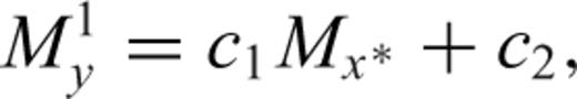
where is the abscissa of the point on the GOR line which is the orthogonal projection of the given point (M_x, _obs, M_y, _obs) and c₁ and c₂ represent the slope and the intercept of the line, respectively (Fig. 1).

Figure 1

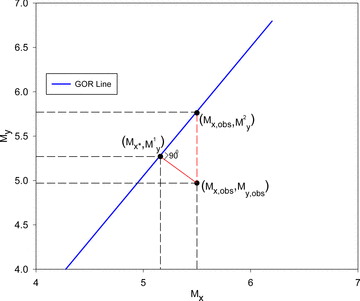
General orthogonal regression relation between M_x and M_y showing the given point (M_x, _obs, M_y, _obs) and the corresponding point (, M¹_y) on the GOR line. The estimate M²_y yielded by eq. (2) for the given point is also shown.

Open in new tabDownload slide

It is pertinent to note that the above GOR relation is commonly used by different researchers by replacing M_x* with M_x, _obs as follows:

2

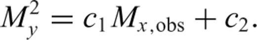
The estimate M²_y given by eq. (2) is different from the actual estimate M¹_y given by the GOR relation (eq. 1), as the abscissa of the projected point on the GOR line, , is different from the abscissa of the given point, that is, M_x, _obs (Fig. 1). Hence, the commonly used form of GOR relation (eq. 2) with c₁ and c₂ of eq. (1) yields biased estimates for M_y, that is the converted magnitude values. The abscissas of the observed and projected points are the same only in case of standard linear regression line which is obtained by minimizing vertical residuals.

Since the ultimate aim of the conversion process is to be able to get a reliable estimate for M_y (e.g. M_w) corresponding to any given value of M_x, _obs (e.g. m_b/M_s), the conversion relation should be expressed in a form where the given value can be substituted directly into the GOR relation with correct slope and intercept. To express the derived GOR relation appropriately in terms of M_x, _obs, a linear relationship needs to be developed between the given values of M_x, _obs and corresponding values, determined by the orthogonal projection of the given points (M_x, _obs, M_y, _obs) on the GOR line as given below.

3

where c₃ and c₄ represent the slope and the intercept of the straight line fit, respectively.

Using eqs (3) and (1), the GOR relation can be easily expressed into an equivalent form as

4

where c₅ = c₁c₃ and c₆ = c₂+c₁c₄. The above relation is referred hereafter as the proposed form of GOR relation for the given set of magnitude pairs (M_x, _obs, M_y, _obs).

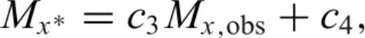
3 Data Set

Body and surface wave magnitudes of earthquakes for the entire globe from the International Seismological Centre (ISC, UK ), database and moment magnitudes from Global Centroid Moment Tensor (GCMT) database () during the period 1976–2007 have been compiled in this study. Body wave magnitudes for 71 339 events, surface wave magnitudes for 70 339 events and moment magnitudes for 27 229 events have been used in all. Some events are seen to be common within different data sets used for deriving relations for conversion of different magnitude types, and similarly within different testing data sets.

4 Conversion of Different Magnitude Types Using Gor Procedure

4.1 Body wave magnitude conversion

For the development and validation of a GOR relationship between m_b and M_w, a data set for 20 466 events with m_b, _obs and M_w, _obs magnitude values has been considered from ISC and GCMT databases for the entire globe for the period 1976–2007 in the magnitude range 4.4 ≤m_b≤ 6.2. This data set has been further subdivided into two subsets with 19 466 randomly selected events included in the first subset and the remaining 1000 events in the second subset. Although the first subset has been used to develop GOR relation, the second subset has been used to test and validate the proposed GOR.

The standard deviations of the measurement errors for M_w and m_b magnitudes are considered as 0.09 and 0.2, respectively, giving error variance ratio (η) as 0.2 (Das et al. 2011). The GOR relation is given below.

5

where m_b* is the abscissa of the point on the GOR line given by the orthogonal projection of the given point (m_b,obs, M_w,obs), R_XY is the correlation coefficient and RMSO is standard deviation of orthogonal errors.

The value of m_b* corresponding to any given point (m_b,obs, M_w,obs) is known by determining the point of orthogonal projection of the given point on the GOR line. The linear relation based on 19 466 values of m_b,obs and corresponding values is given by

6

From eqs (5) and (6), we finally get the GOR relationship for M_w estimates in terms of m_b,obs as given below.

7

This GOR relation and its commonly used form, that is eq. (5) with m_b* replaced by m_b,obs, are shown in Fig. 2(a).

Figure 2

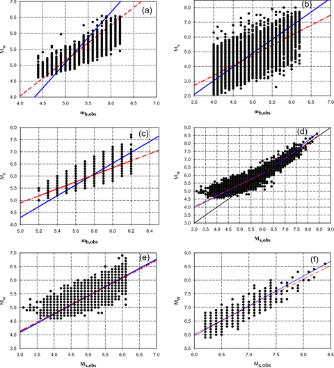
Plots of regression relations using commonly used form of GOR (solid line) and proposed form of GOR (dashed line): (a) between m_b,obs and M_w, (b) between m_b,obs and M_s, (c) between m_b,obs and M_e, (e) between M_s,obs and M_w in the range 3.1 ≤M_s≤ 6.1, (f) between M_s,obs and M_w in the range 6.2 ≤M_s≤ 8.4. A combined plot of M_s and M_w data pairs showing the bilinear trend is also given in (d).

Open in new tabDownload slide

Similarly, a GOR relation between m_b and M_s magnitudes using η= 0.36 (Das et al. 2011) has been developed based on 70 339 data points pairs (m_b,obs, M_s,obs) as given below.

8

The linear relation between m_b,obs and corresponding m_b* values based on 70 339 data points is given by

9

From eqs (8) and (9), we get the following GOR relationship between m_b,obs and M_s as given below.

10

This GOR relation and its commonly used form,that is eq. (8) with m_b* replaced by m_b,obs, are shown in Fig. 2(b).

A GOR relation is also obtained between m_b and M_e with η= 1 (Bormann et al. 2007) based on 739 data points as given below.

11

The linear relation between m_b,obs and corresponding m_b* values for the 739 data points is obtained as follows:

12

From eqs (11) and (12), we get the final GOR relation between m_b,obs and M_e as

13

This GOR relation and its commonly used form given by eq. (11) with m_b* replaced by m_b,obs are shown in Fig. 2(c).

The data shown in the Figs 2(a)–(f) contain measurement errors and the GOR best-fitting lines are drawn based on specific values of error variance ratio (η) between the magnitude types involved. It can be seen that the lines representing the GOR equations developed using proposed methodology are closer to the trend of the data compared to commonly used GOR forms.

An attempt has been made to validate the results of the proposed GOR procedure, using test samples of 1000 (in case of m_b to M_w and m_b to M_s relations) and 100 (in case of m_b to M_e relation) observed events data not used in deriving the GOR relations. Based on a comparison between the absolute average difference and the standard deviation for the corresponding estimates provided by the two GOR forms, it is observed that estimates of the converted magnitudes obtained using the proposed procedure are found to be in better agreement with the corresponding observed values than commonly used GOR methods as shown in Figs 3(a)–(f).

Figure 3

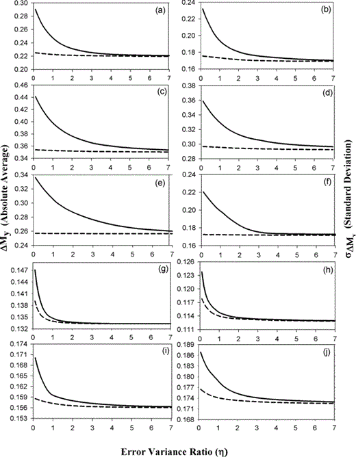
A Comparison of absolute average difference and standard deviation values for the estimates given by the proposed form shown as (dashed lines) and the commonly used form shown as (solid lines) of GOR relations for different η values for various magnitude conversions, (a and b) between m_b and M_w, (c and d) between m_b and M_s, (e and f) between m_b and M_e, (g and h) between M_s and M_w in the range 3.1 ≤M_s≤ 6.1, (i and j) between M_s and M_w in the range 6.2 ≤M_s≤ 8.4.

Open in new tabDownload slide

4.2 Surface wave magnitude conversion

It is observed that the 17 009 global M_s events for magnitude range 3.1 ≤M_s≤ 8.4, considered in this study depict a bilinear trend (Fig. 2d) as was also suggested by Scordilis (2006). Therefore, the magnitude range has been divided into two parts, that is 3.1 ≤M_s≤ 6.1 and 6.2 ≤M_s≤ 8.4, on the consideration that the distribution is linear in these respective magnitude ranges.

For conversion of surface wave magnitudes to M_w, we considered 14 728 events in the magnitude range 3.1 ≤M_s≤ 6.1 and 981 events in the magnitude range 6.2 ≤M_s≤ 8.4. Following the procedure as explained in the previous section, the GOR relation between M_s* and M_w with η= 0.56, the linear relation between M_s* and M_s,obs and the final GOR relation between M_s,obs and M_w for the magnitude range 3.1 ≤M_s≤ 6.1, are as given below.

(l4)

(l5)

and

(l6)

The corresponding relations for the magnitude range 6.2 ≤M_s≤ 8.4 are as follows:

17

18

19

The GOR relations given by eqs (16) and (19) are shown in Figs 2(e) and (f) along with commonly used GOR forms.

For testing these GOR relations for the magnitude ranges 3.1 ≤M_s≤ 6.1 and 6.2 ≤M_s≤ 8.4, we used 1000 and 300 randomly selected events, respectively. It can be seen in Figs 3(g)–(j), that the GOR relations derived in this study using the proposed procedure yield improved M_w estimates compared to the estimates given by their commonly used forms.

5 Validation of Gor Procedure for η Values

The proposed GOR procedure has been further verified for a range of η values from 0.1 to 7.0 based on the comparison of the absolute average difference and the standard deviation for the corresponding estimates provided by the two GOR forms.

In the case of m_b to M_w conversion relation, it is observed that the absolute average difference between the observed and the estimated values of M_w and its standard deviation are significantly lower for the proposed GOR procedure compared to the commonly used form for η values between 0.1 and 2.0 (Figs 3a and b). Similarly, for conversion of m_b to M_s and m_b to M_e, it is found that for η values between 0.1 and 4.0, the proposed GOR procedure yields significantly lower values of the absolute average difference and its standard deviation between observed and estimated values (Figs 3c–f).

For M_s to M_w conversion, the estimates provided by the two GOR forms are found to be almost similar. However, the absolute average difference and standard deviation values are always smaller in case of the proposed GOR procedure (Figs 3g–j).

6 Summary and Conclusions

In this study, we demonstrate a GOR procedure for the conversion of different magnitude types based on events for the whole globe during the period 1976–2007. In this regard, GOR relations have been first derived in terms of the abscissa () of the projected points on the line corresponding to the given data pairs (M_x, _obs, M_y, _obs). The GOR relations in this form have been derived for conversion of m_b to M_w,m_b to M_s and m_b to M_e using ISC data for 19 466, 70 339 and 739 events, respectively. Similarly, the GOR relationships for M_s to M_w conversion have been derived for magnitude ranges 3.1 ≤M_s≤ 6.1 and 6.2 ≤M_s≤ 8.4 using 15 709 M_s events from ISC. These GOR relations have been derived using specific η values as given by Das et al. (2011).

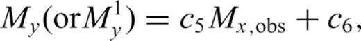
For convenience of estimation of a preferred magnitude type (M_y), the GOR relations are then expressed in a form allowing direct substitution of the observed value of the magnitude (M_x, _obs) as is shown in eq. (4). It is pertinent to note that direct substitution of M_x, _obs, in place of M_x* in the GOR relation given by eq. (1), which is the commonly used form of GOR, shall yield biased estimates since the GOR procedure is based on the minimization of perpendicular residuals instead of vertical residuals. Hence, the use of proper form of GOR relations becomes necessary to obtain accurate estimates.

The validity of the proposed form of GOR relations have been tested based on independent events data not used in developing regression relations for a range of η values from 0.1 to 7.0, by comparing the absolute average difference and the standard deviation for the corresponding estimates provided by the two GOR forms.

In the case of m_b to M_w conversion, the proposed GOR form with η= 0.2, gives the absolute average difference and standard deviation between observed and estimated M_w values as 0.224 and 0.175, respectively, whereas these values obtained by commonly used GOR form are 0.283 and 0.226. The proposed GOR form gives relatively lower values of absolute average difference and standard deviation for a range of η values between 0.1 and 2.0 (Figs 3a and b). For m_b to M_s conversion with η= 0.36, the absolute average difference and standard deviation values of 0.353 and 0.296, respectively, are obtained for the proposed GOR form compared to the corresponding values of 0.423 and 0.347 for the commonly used GOR form. These values are evaluated based on 1000 test events data. It is observed that for m_b to M_s conversion, proposed GOR gives lower values of absolute average difference and standard deviation for η values between 0.1 and 4.0 (Figs 3c and d).

Similarly, for m_b to M_e and M_s to M_w conversions, the proposed GOR form yields lower values of absolute average and standard deviation for the differences between observed and estimated values compared to the commonly used form (Figs 3e and f and g–j).

The GOR procedure demonstrated in this study thus provides an effective way of obtaining improved magnitude conversions that can be applied to obtain homogenized earthquake catalogues for a seismic region. The order of improvement in the estimates, however, depends on the magnitude type and the η value used.

Acknowledgments

The authors are grateful to the reviewers, for their critical reviews and constructive suggestions, which helped improve technical content significantly. The second author is thankful to AICTE, Govt. of India for award of National Doctoral Fellowship.

References