Finite-frequency structural sensitivities of short-period compressional body waves

Summary

1 Introduction

In seismic tomography, the resolution potential of a given data set depends critically on both spatial coverage and frequency content of seismic waves amongst other things. High resolution images of the mantle have been obtained in the past by inverting the global data set of the International Seismological Centre (e.g. van der Hilst 1997; Bijwaard 1998), which contains millions of compressional wave arrival times picked for the most part on short period records. In spite of the tremendous size of this data set, the resolution was still limited by uneven ray coverage, as a large part of the Earth's mantle is poorly sampled, and by the level of noise in traveltime data. With the ever-increasing number of temporary and permanent broadband stations worldwide, spatial coverage and consequently resolution is expected to improve dramatically in many parts of the mantle. To further improve our tomographic images of the Earth's interior, it is now necessary to build high quality global data sets of traveltime and amplitude measurements by exploiting the waveforms of a large number of seismic phases. Such an effort is currently underway, and the results will be reported soon in a forthcoming publication. To fully exploit this new data set, it is also necessary to develop efficient numerical methods to compute the exact sensitivity to 3-D structure of such traveltime and amplitude measurements. This is particularly challenging for the case of P or PKP waves, because the computations must be performed for periods as short as 1 s, around which these waves are best observed on seismic records.

Finite-frequency kernels can in principle be computed exactly in 3-D Earth models (e.g. Tromp 2005; Zhao 2005; Sieminski 2007; Fichtner 2008; Liu & Tromp 2008). However, these approaches require extremely large computational resources even at periods much longer than our target of 1 s, which prevents their application to massive P-wave traveltime data sets. Dahlen (2000) proposed an algorithm based upon far-field asymptotic solutions of the wave equation (ray theory) to make calculations of traveltime kernels for high frequency body waves tractable. A few tomographic studies subsequently used this approach to incorporate 3-D traveltime kernels into global tomography studies (e.g. Montelli 2004). While the asymptotic approach (Dahlen 2000) accounts for finite-frequency effects on traveltimes and amplitudes, it still suffers from important shortcomings. First, ray theory can not be used to describe diffracted waves such as P_diff or S_diff. This considerably limits our ability to image structures in the lowermost mantle, since waves diffracted by the core have the strongest sensitivity to structural heterogeneity at the base of the mantle. Secondly, neglecting the contribution of the near field can potentially bias traveltime sensitivity kernels in the vicinity of sources and stations, as shown by Favier (2004). Thirdly, asymptotic approximations do not fully describe the complexity of wavefields and it is often cumbersome to account for all the seismic phases that can contribute to the observed signal in the time window of interest. Finally, the computation of wave amplitudes with ray theory is difficult and requires interpolation of the spherical velocity model (Calvet & Chevrot 2005). This problem is important because inaccurate seismic amplitudes translate into errors in traveltime sensitivity kernels, and thus into biases in tomographic models. From this short overview, it is clear that there is a need to develop efficient numerical methods for computing exact sensitivity kernels.

A solution to this problem was proposed by Zhao & Chevrot (2011a) who showed that partial derivatives can be expressed as convolutions of the components of two types of strain Green's tensors (SGTs), emanating from the source and back-propagated from the receiver. These SGTs can be precalculated with any simulation method and stored in a database, so that they can be retrieved to compute partial derivatives very efficiently. Zhao & Chevrot (2011b) computed the SGTs by normal-mode summation and showed examples of kernel computations for various seismological observables on both body and surface waves. Because it is difficult to compute spheroidal modes at periods shorter than 8 s, they could only compute body wave kernels at relatively long periods.

Here, we will use the Direct Solution Method (DSM) to compute the SGT database, with the objective of being able to compute sensitivity kernels at periods as short as 1 s. The DSM is a Galerkin method that solves the weak form of the elastic equation of motion in the frequency domain (e.g. Geller & Ohminato 1994; Geller & Takeuchi 1995). By carefully tuning the vertical grid spacing, maximum angular order, and cut-off depth, the calculations can be made very efficient while keeping high accuracy, even at frequencies as high as 2 Hz (Kawai 2006). We first describe this method and derive the expressions of SGTs from the numerical solutions for displacement. We then explain an important improvement of our initial implementation that consists of interpolating SGTs, thereby avoiding the need to compute and store the SGT database in a grid with fine distance and depth sampling rates. This saves storage space and limits the volume of data that needs to be read for computing the sensitivity kernels. Another improvement comes from an adaptive algorithm that determines the domain where the values of the partial derivatives are significant, thereby avoiding the unnecessary computation of the kernels outside the first Fresnel zones. We illustrate our approach by computing Fréchet kernels for the traveltimes and amplitudes of high frequency P, PKP and P_diff phases. Finally, we compute waveform partial derivatives for different parts of the seismic wavefield and demonstrate their potential for high resolution imaging of the deep Earth by migration and waveform inversion.

2 Partial Derivatives Expressed in Terms of Strain Green's Tensors

2.1 Fréchet kernels expressed in terms of strain Green's tensors

The perturbation of the displacement from a source to a receiver due to structural perturbations at can be obtained by the convolution of the forward-propagating field at from and the adjoint (time-reversed back-propagated) field from (e.g. Geller & Hara 1993). In the frequency domain, this can be expressed as

1

where is the i-component of the forward propagated displacement at excited by a source (either a double couple or a force), and is the Green's tensor, that is, the i-component displacement at excited by a unit impulsive force applied in the n-direction at . Note that an asterisk superscript denotes complex conjugation. and are the perturbations to the density and elastic tensor, respectively. 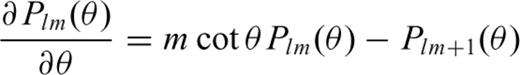The geometry of the locations and in the Earth and their projections onto the surface of the sphere are shown in Fig. 1. Einstein's summation rule is assumed throughout this paper. A comma in the subscript indicates spatial differentiation. For example,

is the local Cartesian derivative. Using the symmetry property of the elasticity tensor

2

and focusing only on the perturbation of the elastic tensor, we can further simplify eq. (1) as

3

where denotes the (i, j)-component of the strain of the forward field

4

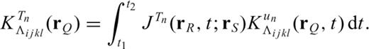
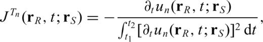
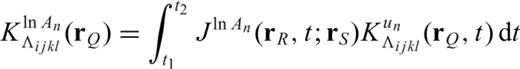
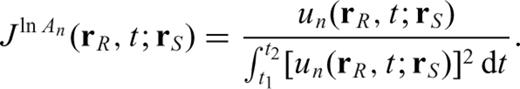
and is the (k, l)-component of the strain associated with the Green's tensor , that is, the single-side SGT defined in Zhao & Chevrot (2011a)

5

1

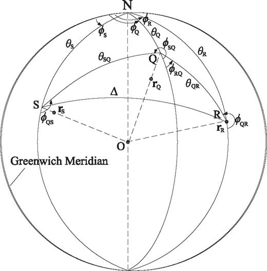
Geometry of the source at , receiver at and an arbitrary location at which the Fréchet kernel is calculated (from Zhao & Chevrot 2011a). s, R and Q are the surface projections of , and , respectively. Here and R coincide, since the receiver is assumed to be on the surface.

Open in new tabDownload slide

The forward strain field ε_ij produced by a moment tensor M_pq at can be expressed as

6

where H_ijpq is the two-side SGT defined in Zhao & Chevrot (2011a).

The DSM accounts for the effect of anelasticity in an exact manner (Fuji 2010). Therefore eq. (3) can be used to model the displacement perturbation due to a general complex perturbation to the elastic tensor, including the effects of perturbations in physical dispersion and attenuation. In this study, however, for simplicity, we only consider elastic perturbations relative to an anelastic reference model, that is, δΛ_ijkl is real and frequency independent.

For the perfectly elastic case, substituting eq. (6) into eq. (3) and transforming it to the time domain, we obtain the same expression of Zhao & Chevrot (2011a,b) for the waveform perturbation density

7

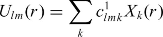
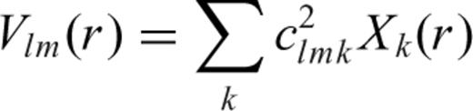
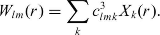
In this expression, is the third-order Single-side Strain Green's Tensor (SSGT) whose elements h_ijk represent the (j, k)-component of the strain field at due to an impulsive point force acting at along direction i-direction. Similarly, is the fourth-order Two-side Strain Green's Tensor (TSGT) whose elements H_ijkl represent the (i, j)-component of the strain field at due to an elementary double couple source M_kl applied at . Note that the symbol * denotes convolution in time. The waveform perturbation density in eq. (7) is the fundamental quantity to consider in the derivation of partial derivatives. For example, the partial derivative of a waveform at location and time t with respect to a perturbation δΛ_ijkl of the elasticity tensor is simply

8

Using the partial derivatives in eq. (8), we can derive the expressions for the Fréchet kernels of any seismic observables derived through linear operations of waveform. For example, the expression of the sensitivity kernel for the traveltime of a seismic phase obtained by cross-correlation of observed and synthetic seismograms in the time interval [t₁, t₂] can be written as (Dahlen 2000)

9

We can taper the time window so that the amplitude of the seismic phase being measured is zero at both ends of the time window, this leads to

10

while the amplitude kernel takes the form:

11

with

12

Therefore, to compute the value of a Fréchet kernel at an arbitrary location, we only need to know the elements of the third-order SSGT h and fourth-order TSGT H.

2.2 P-wave kernels

From now on, we will focus on the computation of kernels for high-frequency P waves. These waves are mostly sensitive to α, the compressional wave velocity. An isotropic elasticity tensor is given by

13

where λ and µ are the Lamé parameters, and δ_ij denotes the Kronecker delta. Substituting eq. (13) into eq. (7) and using the relation between the perturbations of P-wave speed and elastic moduli

14

we obtain the partial derivative of the n-component waveform for α

15

16

where for brevity the spatial and temporal dependence of the SGTs is omitted. From this expression, it can be seen that to compute P-wave kernels we only need the trace of the second-order strain tensor part of SSGT and TSGT at location . In addition, since P waves are generally observed on vertical components, it is sufficient to compute the components of the SSGT h corresponding to n=r.

2.3 Construction of a strain Green's tensor database

The numerical efficiency of our approach relies on the fact that we can evaluate expressions such as (16) by using a pre-calculated database of SGTs. For example, as shown in Fig. 1, if we can calculate in advance the TSGT H for all possible locations of r_S and r_Q and establish a database, then in the evaluation of any Fréchet kernels we can simply retrieve the TSGTs from the database, thus achieving a better efficiency. In general, each element of the TSGT H is a function of six variables: the 3-D coordinates of r_S and r_Q. As a result, the amount of computation and storage for the TSGT database are huge and can only be applied on small-scale studies (e.g. Zhao 2006; Chen 2007). However, for a spherically symmetric Earth model, the TSGT H only varies with four parameters: r_S and r_Q, the arc distance Δ_SQ, and the angle φ_QS. Furthermore, the spherical symmetry leads to the decoupling of the dependence on φ_QS from the other three variables. As a result, we can establish a TSGT database with all its elements sampled for a set of (r_S, r_Q, Δ_QS) values. The dependence on φ_QS, all in the form of its sines and cosines, can easily be taken into account during the kernel calculations.

In actual implementation, the TSGT elements in the database are calculated in a spherical polar system in which r_S is on the north pole and the arc SQ coincides with zero longitude. Then, when we use eq. (16) to compute the kernel, we need to first rotate the coordinate system at r_S by the angle φ_QS. Note that this rotation transforms the last two indices of the fourth-order TSGT, that is,

17

where R is the rotation matrix corresponding to a rotation of angle φ_QS around the vertical axis, and is the TSGT calculated and stored in the database. We thus obtain

18

19

20

21

22

23

In deriving these expressions, the contributions of and have been omitted, because they only contribute to the SH wavefield. Since the TSGT is a two-point tensor, a similar rotation of angle φ_SQ at r_Q is also needed to transform the first two indices of . Therefore, in general both φ_QS and φ_SQ are needed to transform the TSGT in the database to the one used in eq. (16). However, for the vertical-component P waves we consider in this study, terms involving φ_SQ cancel out.

The third-order SSGT h is also a two-point tensor and in practice its database involves its elements sampled on a set of (r_Q, r_R=a, Δ_QR) values, where a is simply the Earth's radius. Similar to the TSGT, coordinate rotations are required at r_Q and r_R to transform the SSGT in the database to that in eq. (16). Again, for vertical-component P waves all terms involving rotation angles cancel out, and we obtain the sensitivity of the vertical P wave to P-wave speed

24

25

26

27

28

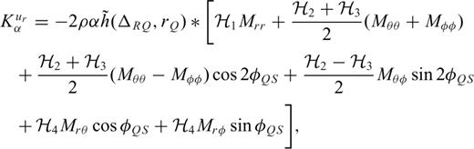
Here, is the trace of strain at distance Δ_QS and radius r_Q produced by an elementary double couple M_rr at radius r_S. Similarly, the other components , and , are for elementary double couple sources M_θθ, M_φφ and M_rθ, respectively. We point out that eq. (24) can be derived from a simplification of the general relations given in the appendices of Zhao & Chevrot (2011a).

In general, as demonstrated by Zhao & Chevrot (2011a), the computation of partial derivatives requires 10 components for and 20 components for . However, for the particular case of P waves, our derivation shows that only one component is actually required for and four components for (that we name ). Therefore, it is possible to design an optimal database of SGTs for the computation of P wave partial derivatives. Another advantage of defining specific databases for each type of seismic phase is that we can fine tune the time (or frequency) and spatial samplings in the computation of the SGTs. We explain in the next section how these strain tensors can be computed with the DSM.

3 Computation of Strain Green'S Tensors with the Direct Solution Method

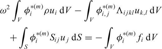
3.1 The direct solution method

We express the displacement as a linear combination of N vector trial functions

29

We use linear spline functions X_k(r) for the vertical dependence of the displacement

30

and complex vector spherical harmonics S¹_lm, S²_lm and T_lm to describe the lateral dependence of the displacement

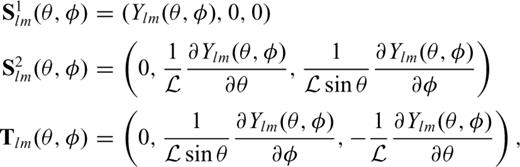
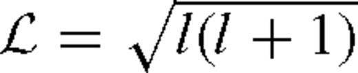where Y_lm(θ, φ) are fully normalized spherical harmonics and (Takeuchi & Saito 1972; Takeuchi 1996). In this vector spherical harmonics basis, the displacement vector is given by

31

where the radial functions are related to the radial trial functions through

32

33

34

The weak form of the equation of motion can be written as

35

with ρ and Λ, respectively the density and the fourth-order elasticity tensor, and f the excitation of the earthquake. Note that DSM can handle attenuation effects with no additional cost. In this expression, superscript * denotes the complex conjugate. By substituting eq. (29) into eq. (35), we obtain the Galerkin weak form of the equation of motion

36

where T is the mass matrix, H is the stiffness matrix, g is the force vector and R is an operator which enforces continuity conditions at fluid-solid boundaries. The elements of the matrices in eq. (36) are given by

37

38

39

40

This equation is directly solved to find the expansion coefficients of displacement contained in vector c.

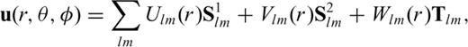
3.2 Computation of strain from the displacement solution

From the solution for displacement obtained using the DSM in eq. (29), we can derive the expressions for the various components of the SGTs. Since we only need the trace of the strain tensor, we need to compute

41

42

43

Note that in these expressions we only kept the contributions of S¹_lm and S²_lm which correspond to the P-SV wavefield and dropped the terms in T_lm which correspond to the SH wavefield. The derivatives of displacement with respect to φ and θ are obtained analytically, using the following identities

44

45

46

To derive derivatives of displacement with respect to the vertical direction, we use a three-point interpolation algorithm (Suetsugu 2005; Kawai & Geller 2010a). Since vertical strain is discontinuous at a discontinuity, we do not mix the displacements in the upper and lower zone when we interpolate. In this paper, for simplicity, we show the strains in the upper zone except the case for the surface.

The Green's functions are calculated for the ak135 reference Earth model (Kennett 1995) with a step of 0.1° in distance, 20 km in depth from the surface down to the bottom of the mantle, and 0.05 s in time, for frequencies up to 1.25 Hz. These Green's functions are then stored on a disk.

4 Interpolation of Green's Functions

While the calculation of partial derivatives with the SGT database approach is very efficient, it is still limited by the number of SGT that must be stored and accessed during execution. Kernels are usually computed in a fine 3-D grid, and we require access to both SSGT and TSGT inside each element of this grid, which means that we must compute and store the SGT with a fine distance sampling. For example, in their computation of traveltime kernels, Zhao & Chevrot (2011b) used a SGT grid with a distance step as small as 0.01° for 8 s period kernels. Such a fine distance sampling requires both a significant volume of storage and reading large flows of input files during the computations. We will now present the results of a first attempt to reduce very significantly the size of the SGT database, while keeping the accuracy of the resulting kernels.

The interpolation of uniformly sampled and non-aliased data is straightforward, and can be performed by a SINC filter in the frequency domain (e.g. Shannon 1949; Unser 2000)

47

48

A 20° distance range is typically considered to perform the interpolations. Since a spatial sampling of Δθ introduces a repetition of the spectrum with period 1/Δθ, spatial aliasing will occur if wavenumbers larger than 1/2Δθ (Nyquist wavenumber) contribute to the signal. In other words, to avoid aliasing, the spatial sampling must satisfy

49

with T_min the shortest period and p_max the maximum slowness in the signal. For example, a 1 s P wave recorded at an epicentral distance of 65° has a slowness of 6.5 s deg⁻¹ and Δθ must be smaller than 0.08°. Obviously, this minimum sampling interval can be doubled if we consider waves with a dominant period of 2 s. Fig. 2(a) shows the results of interpolating 1 s SSGT around an epicentral distance of 65° with a distance sampling of 0.25°. The interpolated traces are distorted by spatial aliasing and cannot be used to compute partial derivatives. For a PKPdf phase at 160° with a slowness of 1.1 s deg⁻¹, the spatial sampling must be smaller than 0.45°. Fig. 3(a) shows the results of interpolating 1 s SSGT around an epicentral distance of 170°. As expected, the interpolated traces are very accurate and it is thus possible to interpolate SGTs to compute PKP partial derivatives from a SGT database computed every 0.25°.

2

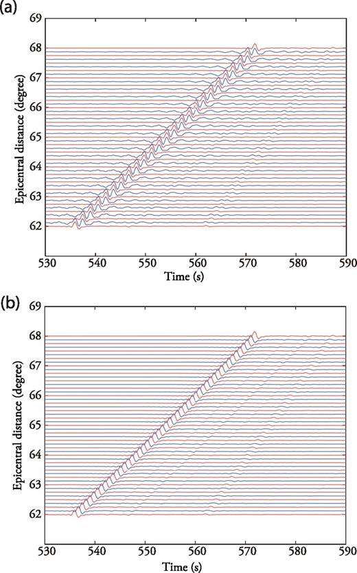
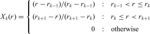
Interpolation of P wave Green's function. The ‘exact’ Single-Side Green's Tensors (red lines) are calculated with DSM at 20 km depth. The blue lines show the interpolated Single-Side Green's Tensors without (top panel) and with (bottom panel) normal move-out corrections for a slowness of 6.51 s deg⁻¹ which corresponds to a P wave observed at an epicentral distance of 65°. All the traces are bandpass filtered between 0.1 and 1.0 Hz. Note the strong spatial aliasing on the interpolated traces when the normal move-out corrections are omitted.

Open in new tabDownload slide

3

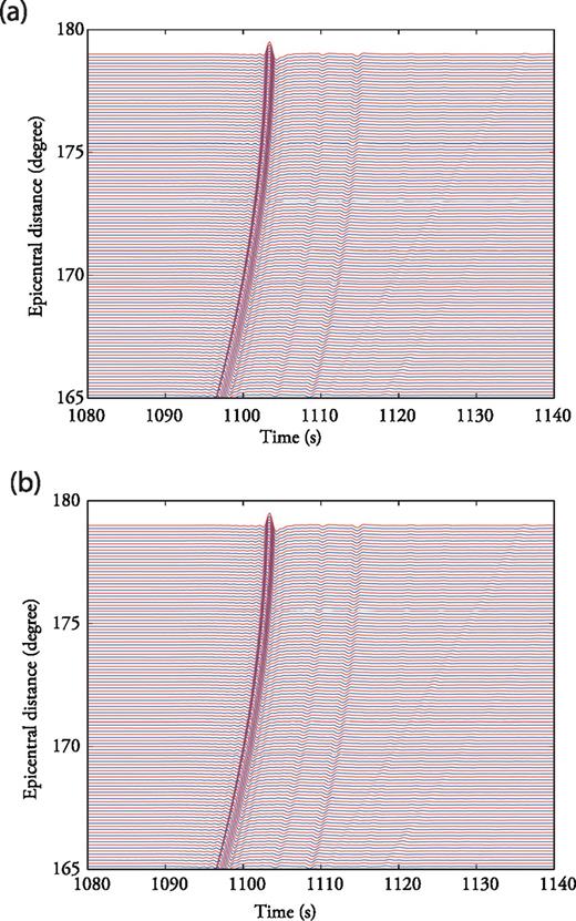
Interpolation of PKPdf wave Green's functions. The ‘exact’ Single-Side Green's Tensors (red lines) are calculated with DSM at 1000 km depth. The blue lines show the interpolated Single-Side Green's Tensors without (top panel) and with (bottom panel) normal move-out corrections for a slowness of 0.24 s deg⁻¹ which corresponds to a PKPdf wave observed at an epicentral distance of 176°. All the traces are bandpass filtered between 0.1 and 1.0 Hz. Note the absence of spatial aliasing on the interpolated traces when the normal move-out corrections are omitted.

Open in new tabDownload slide

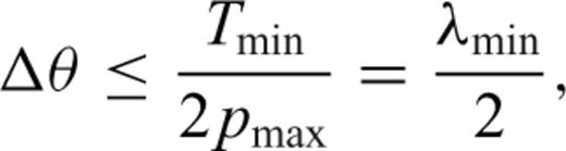
From these simple considerations, it can be seen that the computation of 3-D kernels for teleseismic P waves at frequencies up to 1 Hz and for any distance would require a database of SGTs sampled at about 0.05°. This would already constitute a significant improvement over our preliminary implementation which was based upon a distance sampling of 0.01°. However, it is possible to use a database with an even coarser sampling by reducing the spatial bandwidth before the interpolation. This is done by introducing a move-out correction with a slowness reduction based upon the theoretical ray parameter of the seismic phase. After correction, the seismic waves (for example the P waves) are aligned on all the records and their apparent slowness is then zero. The relation (49) is then satisfied for much larger spatial sampling. As can be seen in Fig. 2(b) the introduction of the normal move-out correction allows us to retrieve perfectly the P wave Green's functions at any intermediate location between the regularly sampled distances in the database. Using this trick, we are thus able to reduce the number of stored SGTs in the database by a factor of 25, which reduces very significantly the size of the database and the volume of input data to be read during the computation of the partial derivatives. The accuracy of the interpolation scheme is demonstrated by a test around the PKP triplication, where the seismic wavefield shows extreme complexities (Fig. 4). We are thus very confident that accurate partial derivatives can be obtained for any type of wave even when using a coarse grid for the SGT database.

4

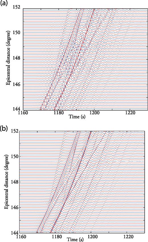
Interpolation of Green's function around the PKP triplication. The ‘exact’ Single-Side Green's Tensors (red lines) are calculated with DSM at 20 km depth. The blue lines show the interpolated Single-Side Green's Tensors without (top panel) and with (bottom panel) normal move-out corrections for a slowness of 2.56 s deg⁻¹ which corresponds to a PKPbc wave observed at an epicentral distance of 150°. All the traces are bandpass filtered between 0.1 and 1.0 Hz. Note the strong spatial aliasing on the interpolated traces when the normal move-out corrections are omitted.

Open in new tabDownload slide

It is interesting to note that the computation of kernels based upon the adjoint method (e.g. Nissen-Meyer et al. 2007a,b) also requires storing the direct and adjoint wavefields on a fine grid. It is likely that the interpolation of strain tensors would also significantly speed up the computations of partial derivatives using the adjoint method.

5 Optimization of the Algorithm

The simplest algorithm to compute 3-D kernels is to define a large domain surrounding the source-receiver great circle plane inside which the values of the derivatives are systematically calculated. However, these values are actually significant only in a much smaller volume, which is defined by the first Fresnel zone. For most classical waves, such as the P or S waves, very small values are also found along the reference path given by ray theory, and the kernels typically have a banana-doughnut shape (Dahlen 2000). This suggests that it is not necessary to compute the partial derivatives systematically inside a large domain, which led us to seek a more efficient and yet simple algorithm.

Our algorithm starts by computing, at each depth, the values of the kernel along the source-receiver great circle plane. We select along this line the points where the absolute value of the kernel exceeds 0.5 per cent of the maximum absolute value to define, at each depth, a mask that will be used for the adjacent planes. This mask is determined to closely follow the shape of the kernel. If the computed values are still above the threshold at one of the edges of the mask, the computation is extended along this direction. This allows the method to adapt to complicated kernel geometries such as the one for PP waves, for example. Fig. 5 shows the example of a kernel for a 10-s period PP wave at 200 km depth computed with this algorithm. As can be seen, this algorithm is able to capture and follow the complex shape of the kernel. This new implementation is interesting because it allows us to diminish the number of computed points by a factor of about 4, without losing any information.

5

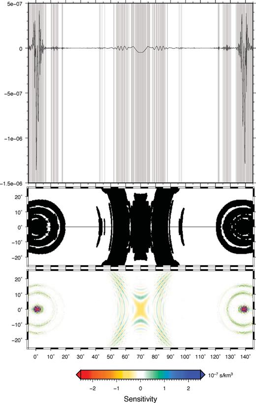
Illustration of the algorithm to compute the sensitivity kernels. In this example, we compute the traveltime sensitivity kernel at 200 km depth for a PP wave bandpass filtered between 0.01 and 0.1 Hz produced by an explosive source at 20 km depth at an epicentral distance of 140°. At each depth, we first detect the position of the significant values of the kernel along the great-circle path (grey regions on the top plot). These domains are then explored and extended along latitudinal lines when moving away from the great-circle path. The kernels are computed only inside these significant domains, marked in black in the middle plot. The bottom plot shows the PP sensitivity kernel at 200 km depth computed with this algorithm.

Open in new tabDownload slide

6 Examples Of 3-D Fréchet Kernels

We will now illustrate our approach by showing examples of traveltime, amplitude and waveform Fréchet kernels for different types of compressional waves. In these computations, we use an explosive source at 20 km depth, and only consider the dependence on °, the P-wave velocity. A finite frequency traveltime anomaly δT is measured by taking the maximum of the cross-correlation function between an observed and a reference seismic phase, inside the time window between t₁ and t₂. This time window is visually or automatically (Maggi 2009) selected by picking the beginning and end of the seismic phase of interest on the synthetic trace. The sensitivity kernels are computed inside a spherical grid with a step of 0.25° in latitude and longitude and 40 km in radius for frequencies up to 1.25 Hz. In all our computations, we considered an explosive source at the north pole and at 20 km depth.

6.1 PKP kernels

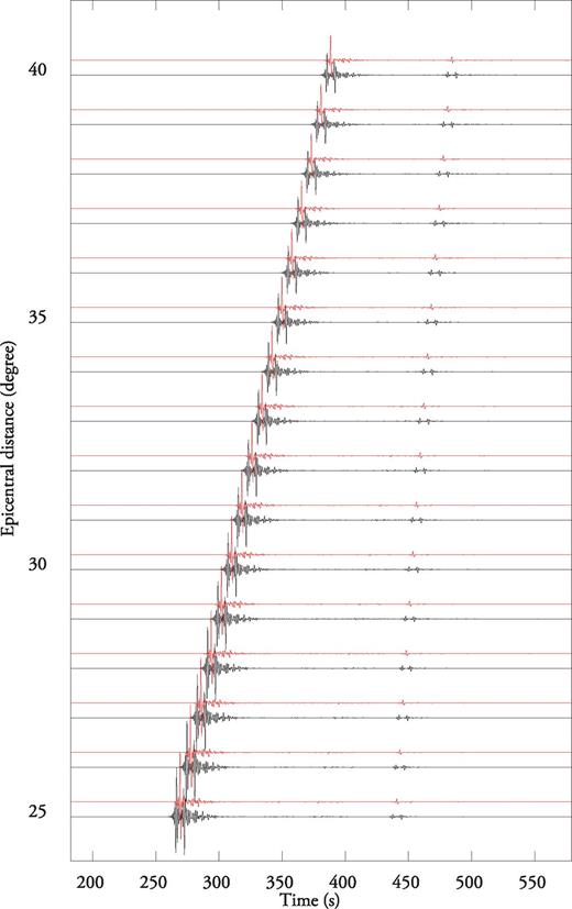
PKP waves are compressional waves that travel through Earth's core. Depending on the epicentral distance, three different PKP branches can be recorded: the PKPab, PKPbc, and PKPdf branches (Fig. 6). Among these, PKPdf is the only one that samples the inner core. The PKPab phase mostly samples the shallow part of the outer core while the PKPbc phase samples the deeper part. The number of PKP phases that can be observed depends on both epicentral distance and depth. At the free surface and for a shallow source, the three phases are simultaneously present only in the distance range 142–155°, often referred to as the PKP triplication. A global data set of PKP traveltimes that could be exploited in the framework of finite-frequency tomography has been recently obtained by Garcia (2006).

6

PKP waveforms (vertical component) with an explosive source at 20 km depth around their triplication. For epicentral distances between 142 and 155°, three PKP branches are recorded: PKPdf, PKPbc, and PKPab. To show the real amplitudes, the traces are not normalized. Note the strong amplification of PKPab and PKPbc phases in this distance range resulting from the B-caustic.

Open in new tabDownload slide

Following the asymptotic approach introduced by Dahlen (2000), Calvet & Chevrot (2005) showed that PKP traveltime kernels are complicated by interference effects between the different PKP branches. In addition, they found that the asymptotic approach suffers from serious limitations because it cannot describe the diffraction of the PKPab phase at the CMB, and because the computation of PKP amplitudes close to the B-caustic breaks down with ray theory. Liu & Tromp (2008) determined PKP kernels from complete forward and adjoint wavefields computed using the spectral element method. They found that PKPab, in contrast to PKPdf, has sensitivity to structure outside the typical banana-doughnut kernel shape, a feature that they did not try to further elucidate. However, their computations were performed for 9 s dominant period PKP waves, well above the periods at which these phases are typically observed.

We show sensitivity kernels only in the mantle part in this paper since no significant heterogeneity is expected inside the outer core. We computed sensitivity kernels for traveltime and amplitude of a 1 s PKPdf wave at a distance of 170° (Figs 7 and 8), using the precomputed SGT database obtained with DSM. Because the PKPdf phase travels faster than the PKPab phase, scattered PKPab waves arrive much later than the PKPdf wave and there is no coupling between the two branches. Consequently, PKPdf kernels display simple and classical shapes, very similar to those of the P wave. In comparison, the traveltime kernel for PKPab at 170° (Fig. 9) appear much more complicated. The strong semi-circular streaks are produced by the contribution of scattered PKPbc and PKPdf phases (and their depth phases), which have very strong amplitudes close to the B-caustic, as can be seen in Fig. 6. However, since their contributions to the PKPab kernels oscillate rapidly, these scattered phases are only sensitive to the very short wavelengths of the power spectrum of the spatial heterogeneity. Another notable feature is that the Fresnel zones of the different PKP waves differ in size and shape, even though the different waves have a similar frequency content. A comparison of traveltime kernels for the three PKP branches at 150° obtained using ray theory (Calvet & Chevrot 2005) and using DSM (this study) is shown in Figs 10 and 11. It is interesting to note that while the PKPdf kernels are very similar, the PKPab and PKPbc kernels show significant differences. These differences are direct consequences of the different approximations involved in ray theory. First, the diffraction of PKPab on the CMB is not accounted for by ray theory and a sharp cut-off is observed at the edges of the shadow zone of PKPab. Second, the amplitudes of PKPab and PKPbc close to the B-caustic determined by ray theory from the geometrical spreading of these phases are incorrect. This introduces strong biases in the traveltime kernels of PKPab and PKPbc. Finally, it can be seen that scattered depth phases contribute to the PKPab kernel. These depth phases are not taken into account in the ray theory computations. This clearly emphasizes another limitation of the asymptotic approach to compute sensitivity kernels, as this requires modelling all the seismic phases that can potentially interfere and contribute to the finite-frequency traveltime measurement in the time window of interest. When the wavefield is complicated, this can be cumbersome and there is always the risk of omitting a phase that makes a significant contribution. Obviously, full waveform modelling approaches such as DSM do not suffer from this limitation.

7

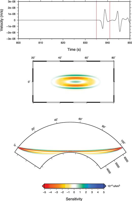
PKPdf synthetic bandpass filtered between 0.1 and 1.0 Hz at 170° epicentral distance with an explosive source at 20 km depth (top panel). Cross-section in the great-circle plane (bottom panel) and map view at 2870 km depth (middle panel) of the traveltime sensitivity kernel for P-wave velocity for a PKPdf phase (the selected window is shown with red lines on the synthetic).

Open in new tabDownload slide

8

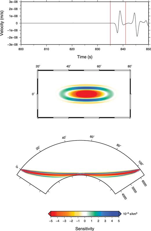
PKPdf synthetic bandpass filtered between 0.1 and 1.0 Hz at 170° epicentral distance with an explosive source at 20 km depth (top panel). Cross-section in the great-circle plane (bottom panel) and map view at 2870 km depth (middle panel) of the amplitude sensitivity kernel for P-wave velocity for a PKPdf phase (the selected window is shown with red lines on the synthetic).

Open in new tabDownload slide

9

PKPab synthetic bandpass filtered between 0.1 and 1.0 Hz at 170° epicentral distance with an explosive source at 20 km depth (top panel). Cross-section in the great-circle plane (bottom panel) and map view at 2870 km depth (middle panel) of the traveltime sensitivity kernel for P-wave velocity for a PKPab phase (the selected window shown as red lines in the synthetic).

Open in new tabDownload slide

10

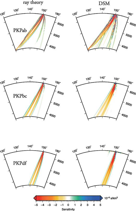
Cross-section comparison between traveltime kernels for P-wave velocity computed with ray theory (left-hand side) and with DSM (right-hand side) for PKPab (top panel), PKPbc (middle panel) and PKPdf (bottom panel) at 150° distance with an explosive source at 20 km depth.

Open in new tabDownload slide

11

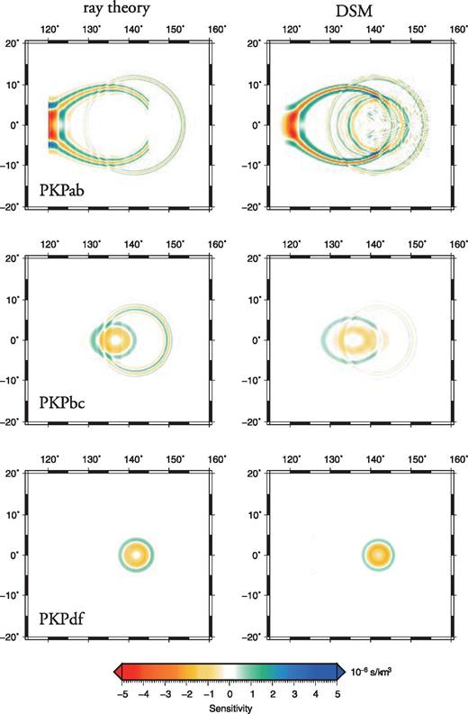
Comparison between traveltime kernels at 2870 km depth for P-wave velocity computed with ray theory (left-hand side) and with DSM (right-hand side) for PKPab (top panel), PKPbc (middle panel) and PKPdf (bottom panel) at 150° distance with an explosive source of 20 km depth.

Open in new tabDownload slide

Since they are mostly sensitive to lowermost mantle structure, PKPab-PKPdf and PKPbc-PKPdf differential traveltimes have been used to constrain the heterogeneities in the D″ layer (e.g. Garcia 2009). Kernels for these differential traveltimes are simply obtained by computing the difference of the kernels corresponding to the two PKP branches involved (Calvet & Chevrot 2005).

6.2 P_diff kernels

P waves diffracted along the core—mantle boundary (CMB) are also very sensitive to heterogeneity at the base of the mantle. However, because these waves cannot be described by ray theory, they have been rarely used in tomographic studies. For example, Karason & van der Hilst (2001) used three P_diff kernels computed by normal mode coupling (Zhao 2000) which were interpolated to determine P_diff kernels at specific distances. This basic approach was the first step to account for the finite Fresnel volumes of diffracted waves, even though the frequency content of the analysed P_diff records and those used in the computed kernels did not match. Figs 12 and 13 show respectively the traveltime and amplitude kernels of a 1 s P_diff at 103° distance. These kernels clearly demonstrate that these waves have a strong sensitivity to heterogeneity in the lowermost mantle, and that the depth of the maximum sensitivity strongly varies as a function of the dominant period of the diffracted wave. Indeed, in their computations based upon normal mode summation down to 8 s, Zhao & Chevrot (2011b) observed that the maximum sensitivity of P_diff waves was about 500 km thick just above the CMB, while in our computations made around 1 s period, we found that the maximum sensitivity is thinner to the CMB (about 100–200 km thick above the CMB). Owing to the variable thickness of the D″ layer and to the strong, small-scale, variability of heterogeneities at the base of the mantle (Garcia 2009), the traveltime and amplitude anomalies of P_diff phases are expected to vary strongly with their frequency content. It is thus crucial to build a high-quality database of finite-frequency measurements of traveltime and amplitude anomalies of diffracted waves and to account for these finite-frequency effects in inversions if we are to improve the resolution of tomographic models at the base of the mantle.

12

P_diff synthetic bandpass filtered between 0.1 and 1.0 Hz at an epicentral distance of 103.3° with an explosive source at 20 km depth (top panel). Cross-section in the great-circle plane (bottom panel) and map view at 2880 km depth (middle panel) of the traveltime sensitivity kernel for P-wave velocity for a P_diff wave The selected window is shown with red lines on the synthetic.

Open in new tabDownload slide

13

P_diff synthetic bandpass filtered between 0.1 and 1.0 Hz at an epicentral distance of 103.3° with an explosive source at 20 km depth (top panel). Cross-section in the great-circle plane (bottom panel) and map view at 2880 km depth (middle panel) of the amplitude sensitivity kernel for P-wave velocity for a P_diff wave The selected window is shown with red lines on the synthetic.

Open in new tabDownload slide

7 Waveform Partial Derivatives

Besides velocity tomography, another approach to image mantle structures is to exploit waves scattered by mantle discontinuities or localized heterogeneities by migration or waveform inversion. In this case, relation (1 or 16) can be used directly to relate the scattered wavefield to the velocity perturbations in the underlying medium. Very often, this is implemented by using simplified migration schemes, relying on asymptotic approximations of the seismic wavefield or by trial and error fitting of 1-D synthetic seismograms. In the following, we examine two different source—receiver configurations that have been used to constrain transition zone discontinuities and D″ layer structure by waveform inversion. Note that for the past several years, three of the authors of the present paper have used these partial derivatives to conduct waveform inversion for the localized 1-D S-wave velocity structure of D″ (Kawai 2007a,b, 2009, 2010; Konishi 2009; Kawai & Geller 2010a,b,c) and for the localized 1-D elastic and anelastic structure of the MTZ (Fuji 2010). Note that Kawai & Geller (2010b) inverted waveform data to directly infer anisotropic structure.

7.1 P waves around the 410-discontinuity triplication

Detailed velocity profiles have been obtained from the exploitation of P wave records in different tectonic regions (e.g. Burdick & Helmberger 1978; Given & Helmberger 1980; Walck 1984), by comparing observed P waveforms to synthetic seismograms computed with a 1-D modelling approach. These models yielded important constraints on the thickness of the high-velocity lid, on the intermittent existence of a low-velocity zone around 150 km depth, and on the depth of transition zone discontinuities, all of which are important clues for understanding mantle dynamics.

We computed the Fréchet kernel given by eq. (16) for the vertical component waveform recorded at a distance of 17° from the source. Fig. 14 shows the values of the partial derivative with respect to ° in the source-receiver plane at different times. The snapshots correspond to times t₁= 236.2 s, t₂= 238.1 s, t₃= 241.0 s and t₄= 243.0 s. The top trace shows the vertical component of the synthetic seismogram around the first P-wave arrival. At this epicentral distance, the P waveform is very complicated. It is a superposition of arrivals that interfere in the time domain. This complexity is produced by the 410 discontinuity, which is responsible for a triplication of the P wave. The first arrival is a P wave that propagates purely in the upper mantle, which is followed by a wave that has been reflected at the top of the 410 discontinuity and by a wave refracted at the discontinuity, that propagates below the 410 discontinuity. These different seismic arrivals can be clearly identified in the waveform Fréchet kernels at onset times t₁, t₂ and t₄. It is interesting to note that the significant values of the waveform partial derivative at this particular distance span a large depth interval, from the surface down to about 600 km depth. This confirms that waveforms recorded around this epicentral distance range are particularly well adapted to constrain upper mantle velocity profiles. The partial derivatives at mid-distance between the source and the receiver at 400 (red cross in Fig. 14) and 500 km depth (blue cross in Fig. 14) are shown in Fig. 15. While sensitivity can be strong at both locations at some particular onsets, the two Fréchet derivatives have very different temporal variations. This demonstrates that a perturbation of seismic velocity inside the mantle has a signature on the seismograms that strongly depends on its location. Waveform inversion identifies these signatures inside observed seismological records to obtain the distribution of velocity perturbations inside Earth's mantle. In contrast to traveltime kernels, for which sensitivity is broadly distributed over the first Fresnel zones, waveform kernels thus have a much better resolution potential but it is essential to consider long time windows to optimize this spatial resolution. In our example, the partial derivatives are computed with respect to a spherically symmetric reference medium. These waveform kernels can be used to migrate seismic waveforms to obtain high resolution images of small-scale mantle heterogeneities and/or seismic discontinuities. Full iterative waveform inversion would require computing SGTs in 3-D models, which is clearly beyond the scope of this study.

14

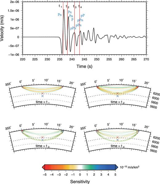
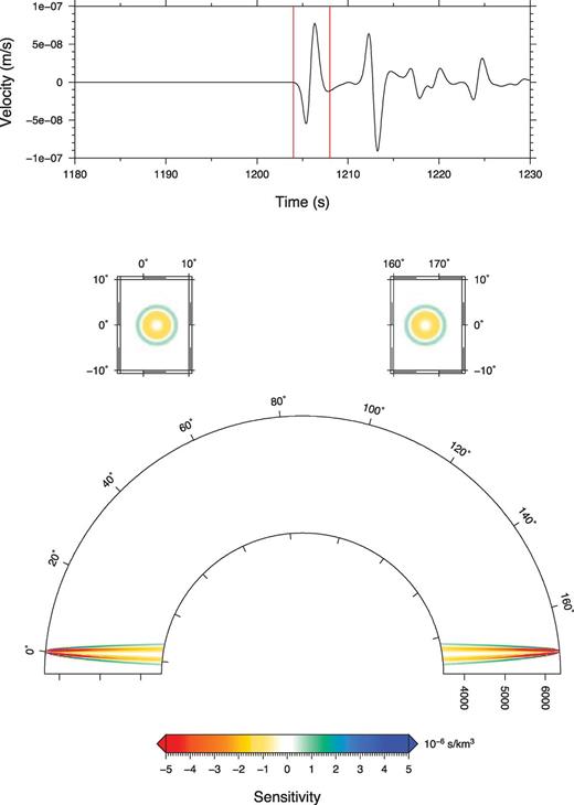
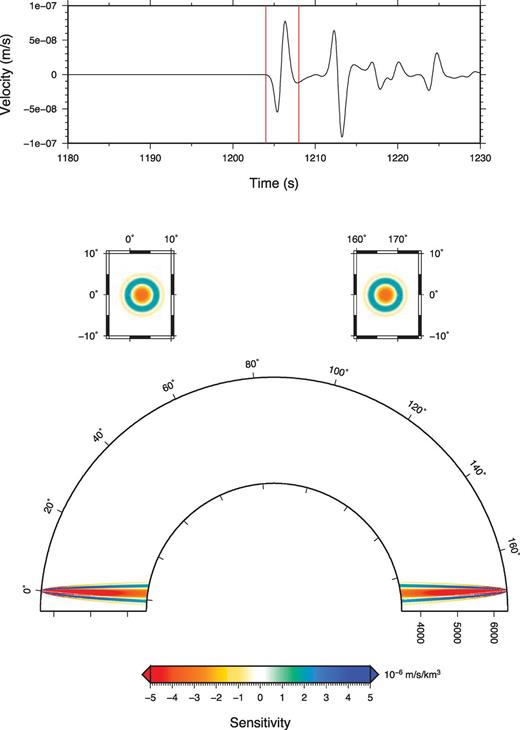
Waveform partial derivatives bandpass filtered between 0.1 and 1.0 Hz for P-wave velocity for a receiver located 17° from an explosive source at 20 km depth at time t₁= 236.2 s, t₂= 238.1 s, t₃= 241.0 s and t₄= 243.0 s. The top trace shows the vertical component of a synthetic seismogram at a receiver located 17° from the source.

Open in new tabDownload slide

15

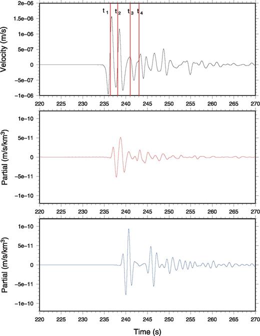
Waveform partial derivatives for P-wave velocity at a point located at 8.5° from the source at 20 km depth at 400 km depth (red) and at 500 km depth (blue). The signals were bandpass filtered between 0.1 and 1.0 Hz. The position of these points are marked with the red and blue crosses in Fig. 14. The top trace shows the synthetic seismogram at a receiver located 17° from the source.

Open in new tabDownload slide

7.2 PcP precursors

The base of the mantle is another part of the Earth's interior that has also been extensively studied by waveform inversion. For example, for epicentral distances between 50 and 90°, in the time interval between P and PcP waves, it is possible to detect PcP precursors corresponding to waves reflected on top of an ultra low velocity layer (e.g. Persh 2001) or scattered by strong heterogeneities in the D″ layer (e.g. Freybourger 2000; Kito & Krüger 2001).

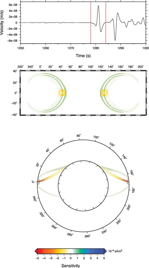
Fig. 16 shows snapshots corresponding to times t₁= 670.0 s, t₂= 678.6 s, t₃= 684.2 s and t₄= 691.7 s, for the partial derivative , computed for a receiver located 70° from the source. The top trace shows the vertical component of the synthetic seismogram around the PcP arrival. The partial derivatives at t=t₁ and t=t₂ clearly show that the sensitivity is concentrated inside the first Fresnel zone of the P wave. The partial derivative at t=t₄ shows some sensitivity inside the Fresnel zone of the PcP wave, but significant sensitivity is also observed at the top of the lower mantle. This suggests that scattering at the top of the lower mantle could also produce a signal in the PcP precursor time window. This can be seen in Fig. 17 where we have plotted the SSGT and TSGT at 940 km depth at mid distance between the source and the receiver. The P waves on each component arrive around 340 s, which means that P waves scattered in this part of the mantle will indeed arrive between the P and PcP waves. The values of the partial derivatives in the mid-mantle are actually larger than those in the bottom part of the lower mantle. Scattered waves resulting from P-P scattering on heterogeneities in the mid-mantle travel through a caustic, and their waveforms are thus expected to be the Hilbert transform of either the direct P wave or the PcP wave. Interestingly, such a difference in waveform has been observed by Freybourger (2000), which could suggest that the PcP precursors that they detected for paths going from Kuril Islands earthquakes to stations in western Europe are actually located in the mid-mantle and not at the base of the mantle.

16

Waveform partial derivatives bandpass filtered between 0.1 and 1.0 Hz for P-wave velocity for a receiver located 70° from the source whose depth is 20 km at time t₁= 670.0 s, t₂= 675.5 s, t₃= 678.6 s and t₄= 692.0 s. The top trace shows the vertical component of a synthetic seismogram at a receiver located 70° from the source.

Open in new tabDownload slide

17

Single-Side Green's Tensors (red lines) and Two-Side Green's Tensors (black lines) at 940 km depth calculated up to 1.25 Hz and filtered between 0.1 and 1.0 Hz for an explosive source at 35° distance. The direct P wave arrives around t= 340 s.

Open in new tabDownload slide

8 Conclusions

We have developed an efficient method to compute accurate 3-D partial derivatives for delay-time, amplitude and waveform anomalies with respect to P-velocities up to 1 s period. This method relies on the exploitation of a precomputed database of SGTs that are calculated with the DSM. To be able to compute kernels for high-frequency teleseismic P waves, we introduced several improvements to the original implementation by Zhao & Chevrot (2011a,b). First, we derived the specific forms of the Green's tensors that are involved in the computation of P wave kernels. This allowed us to reduce drastically the number of SGT components that need to be computed and stored: from 10 to 1 for SSGT, and from 20 to 4 for TSGT. Second, to limit the size of the SGT database, we showed that it is possible to obtain accurate results by interpolating SGTs computed in a coarse grid. Compared to our initial implementation, we were able to reduce the size of the SGT database by a factor 25 without loss of accuracy. This considerably speeds up the computations. Finally, we have optimized the algorithm to compute the values of partial derivatives only where they are significant. This reduces the number of computations by a factor 4. The combination of these different optimizations now allows us to compute partial derivatives for high-frequency teleseismic body waves with very modest computer resources. It takes around 64 days on a single processor to compute P-wave SGTs (1 SSGT and 4 TSGTs) with a length of 1638.2 s up to 1.25 Hz for a grid sampling of 20 km along the vertical dimension and 0.2° along distance. Storing those SGTs requires around 5 Gb of disk space. These numbers are considerably reduced when performing computations at lower frequencies. For example, the same computation would take only 16 days for a frequency cut-off of 0.625 Hz. Once the SGTs are obtained, the computation of a 1 Hz PKP kernel takes around 30 min on a single processor. Using a moderate size cluster, our approach makes finite-frequency tomography feasible, even on rather large data sets.

We have computed traveltime and amplitude kernels for PKP phases up to 1 s period. We found that PKPab and PKPbc kernels show significant differences compared to those computed with the asymptotic forms of the Green's tensors by Calvet & Chevrot (2005). This clearly demonstrates the limitations of the asymptotic approach introduced by Dahlen (2000) to compute sensitivity kernels, even in the high frequency limit where ray theory is expected to give satisfactory solutions to the wave equation. Our approach also allows an efficient computation of waveform partial derivatives. Such quantities will be most useful for waveform inversion of high-frequency teleseismic P wave fields. For example, scattering points located at 400 and 500 km depth have very different temporal contributions to the waveform signal recorded at 17°. This clearly demonstrates that waveform inversion has the potential to resolve heterogeneities with a fine resolution, even with a limited number of records. In comparison, the sensitivity is more broadly distributed in traveltime kernels, and a fine spatial resolution can only be obtained with a very good path coverage. The waveform partial derivatives computed in the spatial and temporal window corresponding to PcP precursors show a complex distribution of sensitivity. In particular, sensitivity is particularly strong in the mid-mantle, way above the base of the mantle where all studies placed the origin of these PcP precursors. In studies of deep Earth structures, it is thus important to consider accurate and complete partial derivatives, which are often complex, and sometimes counter-intuitive. Simple interpretations of seismological records based upon 1-D modelling and/or asymptotic theory can sometimes be seriously misleading.

Acknowledgments

The authors thank Marie Calvet for discussions about the PKP kernels, Tarje Nissen-Meyer for discussions about the kernel calculation in general, and Vadim Monteiller for fruitful discussions about SGT calculation. KK is supported by a JSPS Fellowship for Young Scientists. This study was funded by the ANR-blanc project PYROPE (ANR-09-BLAN-0229) and also was supported by a grant from the JSPS (No.22540433). LZ is supported by a Career Development Award of Academia Sinica in Taiwan.

References