


Summary
We investigate the effect of azimuthal anisotropy on coupling between spheroidal and toroidal modes at frequencies below 4 mHz after large earthquakes of Mw > 7.8, based on the seismic records from Broad-band Array in Taiwan for Seismology stations. Strong coupling of 0S25–0T25 is widely observed at Taiwan Island, but Earth's rotation cannot cause coupling between 0S25 and 0T25 according to coupling selection rules. Different from the Coriolis coupling, the anisotropic coupling of 0S25–0T25 becomes notable only when stations close to nodal lines of 0S25, and the coupling attenuates so rapidly that it is notable on the spectra of 18–24 hr vertical-component records. Modelling indicates that local azimuthal anisotropy is the most possible cause for the strong coupling. The abnormally strong coupling of 0S20–0T21 observed at Taiwan Island also shows similar characteristic of nodal nature and fast attenuation, suggesting local azimuthal anisotropy as the dominant factor for the coupling rather than the Earth's rotation, isotropy and transverse isotropy. Our estimation of sensitivity kernels indicates that the coupled modes 0S20–0T21 and 0S25–0T25 show peak sensitivity to azimuthal anisotropy at depth of 400–650 km, suggesting that the strong coupling may be explained by the presence of azimuthal anisotropy in the upper-mantle transition zone beneath Taiwan Island. The east-dipping Eurasian slab and the north-dipping Philippine Sea Plate beneath the Taiwan orogen are responsible for the formation of the anisotropy.
1 Introduction
Azimuthal anisotropy is seismic anisotropy with a horizontal axis of symmetry, which affects the propagation of body and surface waves as well as the free oscillations of the Earth. Hess (1964) first observed azimuthal anisotropy through the azimuthal dependence of Pn velocities in the Pacific Ocean. Since then, it has been found at various regions in the uppermost mantle, using seismic investigation such as shear wave splitting (e.g. Mitchell & Helmberger 1973; Silver & Chan 1991; Vinnik 1992) and surface wave dispersion measurements (e.g. Forsyth 1975; Montagner & Tanimoto 1990).
Seismic investigations for azimuthal anisotropy in the transition zone of the upper mantle at a depth range of about 410–660 km, however, are quite difficult because fundamental surface waves have poor sensitivity in this range and teleseismic body waves have a very low depth resolution. In body wave studies, comparisons of shear wave splitting from core phases and deep local S phases or converted phases sometimes turn up evidence for splitting associated with azimuthal anisotropy in the transition zone (e.g. Fouch & Fischer 1996; Vinnik & Montagner 1996; Vinnik 1998). Wookey (2002, 2003) and Chen & Brudzinski (2003) use modelling to infer anisotropy in the transition zone beneath the Tonga–Kermadec subduction zone when they detected large S-wave split time, but Saul & Vinnik (2003) argued that S–P conversions near the surface may contaminate the shear wave splitting analysis and hence the inference of transition zone anisotropy. In surface wave studies, Trampert & van Heijst (2002) proved that toroidal overtones show strong sensitivity to azimuth elastic parameter in 400–660 km depth, and thus infer global distribution of azimuthal anisotropy in the transition zone.
Theoretical studies have shown that the azimuthal anisotropy in Earth's upper mantle can cause spheroidal–toroidal normal modes coupling (S–T coupling). Park & Yu indicated that a few per cent perturbations of azimuthal anisotropy on P and S-wave speeds could cause S–T coupling, and thus generate observable “quasi-Love” (QL) waves on vertical component of seismic data in the frequency band of 0–20 mHz (Park & Yu 1992; Park 1993; Yu & Park 1993). Isotropic and radially anisotropic structure may induce coupled modes nSl–n′Tl′ in the upper mantle (e.g. Beghein 2008). Nevertheless, some previous theoretical studies have shown that azimuthal anisotropy is much more ‘efficient’ than isotropy and radially anisotropy for generating QL waves through S–T coupling (Park & Yu 1992; Park 1993; Yu & Park 1993; Yu 1995; Oda & Ohnishi 2001; Oda 2005; Rieger & Park 2010). Using earth model and synthetic tests, Oda (2005) demonstrated that S–T coupling by azimuthal anisotropy can generate significant quasi-toroidal modes on vertical component at frequencies below 3 mHz, but isotropic lateral structure could hardly do this.
Resovsky & Ritzwoller (1998) estimated degree 2 structure coefficients for fundamental modes by observations of 11 coupled modes 0Sl–0Tl+1 below 3 mHz. Comparing these coupling coefficients to the predictions of mantle models, data-to-model differences are unusually large relative to the differences for self-coupling coefficients of the same degree and depth sensitivity. Such large differences may be explained well when anisotropy effects are taken into account (Beghein 2008). The low-frequency anisotropic S–T couplings are sensitive to anisotropic lateral structures throughout most of the mantle, and their energy are mostly situated above approximately 1200 km depth, and therefore, these coupling data have the potential to constrain transition zone anisotropy (Beghein 2008).
Some fundamental principles of geophysics for generating anisotropic S–T coupling are understood through modelling coupled modes. However, it has been thought impossible to directly observe coupled modes 0Sl–0Tl+1 at frequencies below 3 mHz, because such S–T coupling caused by Earth's rotation is strong (Masters 1983). The only exception is that Hu (2009) directly observed significant anisotropic coupling at the seismic stations close to the equator after the 2004 and 2005 great Sumatra earthquakes. It is because that both stations and seismic sources are close to the equator, and thus rotational effects on S–T coupling are negligible when surface waves propagate along near-equatorial paths. The results of their investigation are that the anisotropic coupling are observable at stations close to the nodal lines of harmonics of spheroidal modes, and are notable in the early time after origin time. This characteristic can discriminate anisotropic coupling from rotational coupling in seismic observations.
Taiwan is ideal place for study of anisotropic S–T coupling as it is an island with complicated upper-mantle structures, which caused by the active oblique collision between the Eurasian and the Philippine Sea plates, and it owns dense seismic network that is able to observe normal modes. The purpose of this paper is to analyse coupled modes caused by anisotropy and to demonstrate that the signal of azimuthal anisotropy in the coupling of normal modes can help us constrain anisotropy in the upper-mantle transition zone beneath Taiwan Island.
2 Data and Modelling
Seismic data records used in this study mainly come from the Broad-band Array in Taiwan for Seismology (BATS). Fig. 1 shows the distribution of BATS stations used in this study. Some seismic records from Incorporated Research Institutions for Seismology (IRIS) data management centre and Full Range Seismograph Network of Japan (F-net) are also included in this study. We focus on long-period normal modes excited by seven earthquakes of Mw > 7.8 (Table 1). Data records after these events have sufficient quality to observe normal modes with high signal-to-noise ratios in the frequency band of 1.5-4.0 mHz within 48 hr.
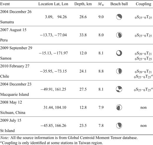
Seismic events concerned by this study.
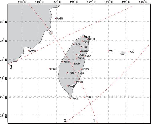
Map of the Taiwan region showing the distribution of seismic stations from BATS and F-net and IRIS DMC. Dashed curves indicate some nodal lines of  : (1) the nodal line with the radius of 160.56° for the 2007 August 15 Peru earthquake; (2) the nodal line with the radius of 160.56° for the 2010 February 27 Chile earthquake; (3) the nodal line with the radius of 82.94° for the 2004 December 23 Macquarie earthquake.
3 Observations
3.1, Observations of coupling 0S25–0T25
Anomalous S–T coupling are often widely observed at seismic stations on Taiwan Island. We first present observations from the 2004 December 26 Sumatra earthquake (Mw= 9.3) recorded at 15 seismic stations of Taiwan in Fig. 2. Amplitude spectra of the vertical component records show small peaks in the frequency band 3.3–3.4 mHz. Close inspection of the vertical component spectra expectedly reveals strong coupling between 0S25 and 0T25. The spectral peak of 0S25 significantly deviate from its theoretical position and quasi-0T25 is obviously present on the spectra. Note that Earth's rotation cannot cause the coupling between 0S25 and 0T25 according to the angular selection rule for coupled multiplets (e.g. Dahlen & Tromp 1998; Zürn 2000). Coupled modes 0S25–0T25 are remarkable at central and northern Taiwan, with characteristic of very small amplitude of 0S25. At stations of central Taiwan, such as NACB and SSLB, the spectral peak of 0S25 is even smaller than that of quasi-0T25. However, we note that high amplitude of 0S25 and no sign of 0S25–0T25 coupling are observed at YNK and IGK, two stations of F-net, although the two stations are close to the northern coast of Taiwan (see Fig. 1). This suggests that 0S25–0T25 coupling observed at stations of BATS is related to the local anisotropic structure near Taiwan Island.
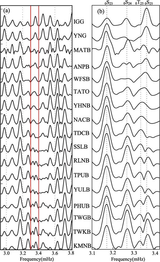
The section of vertical-component spectra at stations in the Taiwan region after the 2004 December 26 Sumatra earthquake. (a) Amplitudes are small in the band of 3.3-3.4 mHz (within the red lines). (b) The magnification of spectra in the band 3.1-3.4 mHz displays significant coupled modes 0S25-0T25. Hanning-tapered Fourier transform is applied to 18-hr time-series, which start at 1000 s after the origin time. Dot lines indicate the theoretical frequencies of normal modes from the PREM model. Labels denote observing site codes.
We explore the spectra around 0S25 recorded at TWKB, SSLB, NACB and WFSB, which are representative stations located at southern, central and northern Taiwan, respectively. We make a comparison among the vertical spectra of 18, 24 and 36 (or 48)-hr records in Fig. 3. The spectra around 0S25 are quite different at the four stations, suggesting that local anisotropy is responsible for strong coupling of 0S25–0T25. Fig. 4 compares the vertical and horizontal spectra at the four stations. 0S25 has small vertical amplitude, but it has very large amplitude on the radial component. In fact, its radial amplitude is the largest one below 3.5 mHz. We note that the radial and transverse spectra are similar around 0S25 at two nearby stations SSLB and NACB, but their vertical spectra are quite different. This observation suggests the presence of strong lateral gradient of anisotropy beneath central Taiwan.
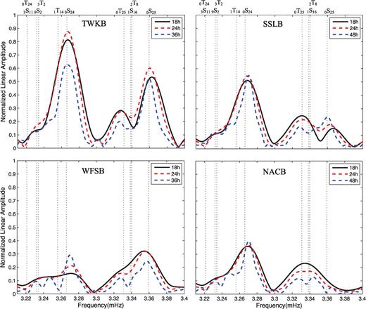
Comparisons among the spectra of 18, 24 and 36 (or 48)-hr vertical component records at BATS stations after the 2004 December 26 Sumatra earthquake. Coupled modes 0S25–0T25 show highest resolution in the spectrum of 18-hr records, indicating a rapid attenuation of the coupling process.
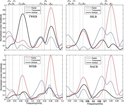
Comparison among 24-hr vertical, radial and transverse spectra at BATS stations after the 2004 December 26 Sumatra earthquake. Coupled mode 0S25 has the largest peak on the radial spectra in the frequency band of 0.3–3.8 mHz. Note that at two nearby stations SSLB and NACB, the radial and transverse spectra are similar around coupled modes 0S25–0T25 but their vertical spectra are quite different, suggesting that lateral gradient of local azimuthal anisotropy is responsible for strong coupling of 0S25–0T25 .
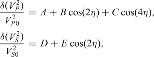
Both radially and azimuthal anisotropic structure can generate S–T coupling. The radially anisotropy causes nSl–n′Tl′ coupling under condition that l+l′+s is odd (s is Earth structural degree), whereas the azimuthal anisotropy causing S–T coupling does not depend on the parity of l+l′+s (e.g. Dahlen & Tromp 1998; Beghein 2008). It seems that azimuthal anisotropy is a more efficient structure than radially anisotropy for generating S–T coupling. In fact, previous studies have demonstrated with Earth's models that S–T coupling is most efficient generated by the presence of azimuthal anisotropy rather than that of isotropy and radial anisotropy (Park & Yu 1992, 1993; Yu & Park 1993). We further demonstrate that azimuthal anisotropy plays a leading role for generating S–T coupling by modelling coupled modes 0S25–0T25 recorded at SSLB. The synthetic coupled modes 0S25–0T25 are computed on the PREM model, where we add elastic perturbations of isotropy, azimuthal anisotropy and radially anisotropy, respectively. We take the global CMT solution as a double-couple point source and compute synthetic coupled modes using the Galerkin method (e.g. Gilbert & Dziewonski 1975; Park & Gilbert 1986). Only fundamental spheroidal–toroidal modes are included in computation. In the case of isotropy and azimuthal anisotropy, we assume that isotropic or anisotropic perturbations are in the upper mantle from the Moho discontinuity to 1000 km depth and they are restricted to the band reaching from 20°N to 24.5°N. When the anisotropy is placed in the band, the fast axis is set to be oriented parallel to the equator. We set parameters B, C and E in (1) equal to 0.1, and A and D equal to 0.0 for the azimuthal anisotropic perturbations, which represents a 10 per cent peak variation in anisotropic wave speed. For the isotropic perturbation in the band, we set A and D equal to 0.1 but B, C and E equal to 0.0, which represents a 10 per cent perturbation in isotropic wave speed. In the case of radially anisotropy, we only add S-wave speed perturbations related to parameters N and L to the upper mantle of PREM model, and radially divide the upper mantle in four layers. The top and bottom depths of these layers are, in kilometres, (24, 120), (120, 220), (220,400), (400, 660). The modelling results are shown in Fig. 5(a). It is easily observed that significant coupling of 0S25–0T25 occur in the presence of azimuthal anisotropy.
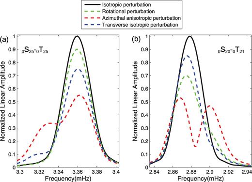
(a) Synthetic spectra of coupled modes 0S25–0T25 recorded at station SSLB after the 2004 December 26 Sumatra earthquake. (b) Synthetic spectra of coupled modes 0S20–0T21 recorded at station SSLB after the 2010 February 27 Chile earthquake. The spectra are computed for a 18-hr record length which is tapered by using a Hanning window.
To investigate the nodal feature of 0S25–0T25 coupling, we present another example from the 2007 August 15 Peru earthquake (Mw= 8.0) recorded at Taiwan Island in Fig. 6. Coupled modes 0S25–0T25 are again remarkable at central Taiwan, with the characteristic of small amplitude of 0S25. Comparisons between vertical spectra of 18 and 48 hr records at RLNB, TPUB and YULB show fast attenuation of the coupling. According to the previous studies, the S–T coupling caused by azimuthal anisotropy is best observed at station near the minima of Rayleigh source-radiation or the nodal lines of spheroidal mode (Oda 2005; Hu 2009). The nodal lines of spheroidal mode  for a point seismic source on a spherical earth are determined by function
  , where
  is normalized associated Legendre function and θ are angular distances from the epicentre to nodal lines. For m= 0, the nodal lines (or antinodal lines) for a point source are estimated by cos((l+1/2)θ-45°) = 0 (or = 1), and thus the nodal lines of
  are a set of small circles on the Earth, with their centre at epicentre and radiuses of θ. The seismic source of the 2007 Peru earthquake is very far away from Taiwan Island, which can be taken as a point source for BATS stations. We note that the nodal line of
  with the radius of 160.56° passes through central Taiwan, but it is little far away from stations KMNB, YNK and IGK (see the line in Fig. 1). This causes small amplitude of 0S25 and strong coupling of 0S25–0T25 at central Taiwan stations, such as at SSLB, TPUB and YULB, but large amplitude of 0S25 and no sign of the coupling at KMNB, YNK and IGK (see Fig. 6a).
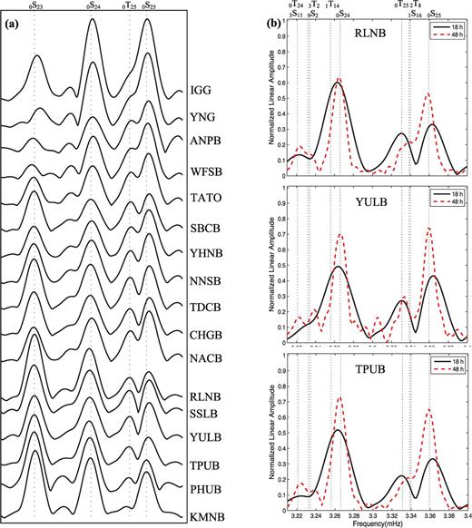
(a) The 18-hr vertical spectra at seismic stations in the Taiwan region showing significant coupling of 0S25–0T25 after the 2007 August 15 Peru earthquake. (b) Comparison between 18- and 48-hr vertical spectra at three BATS stations. Hanning-tapered Fourier transform is applied to time-series, which start at 1000 s after the origin time.
To further demonstrate the nodal nature of anisotropic coupling of 0S25–0T25, we present more examples in Fig. 7. Significant coupling of 0S25–0T25 is remarkable at the central Taiwan station SSLB in our previous examples. However, Fig. 7(a) shows that no sign of 0S25–0T25 coupling occurs at SSLB but it is remarkable at KMNB after the 2004 December 23 Macquarie earthquake (Mw= 8.1). We note 0S25 at SSLB has large amplitude and the nodal line of  with the radius of 82.94° is far from SSLB but very close to KMNB (see Fig. 1). The similar case presented in Fig. 7(b) is that coupled modes 0S25–0T25 do not occur at SSLB but is significant at TWKB, the southernmost station of Taiwan, after the 2010 February 27 earthquake (Mw= 8.8), as the nodal line of
  with the radius of 160.55° is close to southern Taiwan but far from central Taiwan (see Fig. 1). The two examples indicate that even if local azimuthal anisotropy exists beneath seismic stations, significant anisotropic coupling cannot be observed when the stations are far from nodal lines of spheroidal modes.
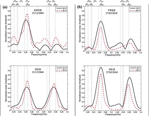
Examples demonstrating the nodal nature of anisotropic coupling of 0S25–0T25 at Taiwan Island. (a) Coupled modes 0S25–0T25 are well observed at KMNB but not at SSLB after the 2004 December 23 Macquarie earthquake, as the nodal line of  with the radius of 82.94° is very close to KMNB but a little far from SSLB (see the nodal line in Fig. 1). (b) Coupled modes 0S25–0T25 coupling are well observed at TWKB but not at SSLB after the 2010 February 27 Chile earthquake, as the nodal line of
  with the radius of 160.55° is close to TWKB but far from SSLB (see the nodal line Fig. 1).
Fig. 8 shows that both SSLB and LSA are very close to the nodal line of  with the radius of 160.56° for the 2007 August 15 Peru earthquake. We note that coupled modes 0S25–0T25 with low amplitude of 0S25 is significant at SSLB. In contrast, there is no coupling at LSA, a seismic station located at Tibet of China. This comparison indicates that the local anisotropy rather than the globe anisotropy causes the 0S25–0T25 coupling at Taiwan Island.
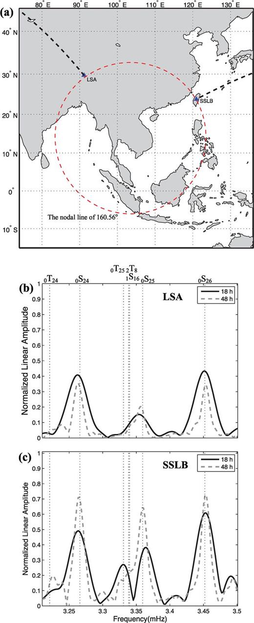
(a) Map showing that stations LSA and SSLB are very close to the nodal line of  with radius of 160.56° for the 2007 August 15 Peru earthquake. The bold dashed lines are the great circle paths for LSA and SSLB. (b) No coupling of 0S25–0T25 is observed at LSA. (c) Coupled modes 0S25–0T25 are significant at SSLB. Hanning-tapered Fourier transform is applied to 18 hr time-series, which start at 1000 s after the origin time.
3.2,Observations of coupling 0S20-0T21
Another typical case of anomalous S-T coupling widely observed at Taiwan Island is coupling between 0S20 and 0T21. Fig. 9(a) shows significant coupled modes 0S20-0T21, with very small amplitude of 0S20, are observed at BATS after the 2010 February 27 Chile earthquake (Mw= 8.8). The coupling is very strong at stations located at central and northern Taiwan, such as TDCB, SSLB and RLNB, and the amplitude of 0S20 is obviously smaller than that of quasi-0T21 at these stations. We note that nodal line of  with the radius of 164.57° is near these stations.
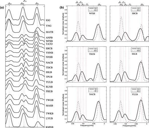
(a) The 18-hr vertical spectra at stations in the Taiwan region showing significant coupled modes 0S20-0T21 after the 2010 February 27 Chile earthquake. (b) Comparison between the 18-hr and 48-hr vertical spectra at six BATS stations. Coupled modes 0S20-0T21 are very strong in the 18-hr spectrum but not identified in the 48-hr spectrum, indicating a rapid attenuation of the coupling process. Hanning-tapered Fourier transform is applied to the records, which start at 1000 s after the origin time.
The Earth&s rotation may also generate coupling between 0S20 and 0T21. However, we note that in Fig. 9(a) coupled modes 0S20-0T21 does not occur at KMAN, MATB, YNK and IGK. The four stations are apart from Taiwan Island about 100-200 km and their azimuths of epicentre station are approximate to these of stations at Taiwan Island. Therefore, the effects of Coriolis force on normal modes at the four stations are almost the same as those at Taiwan Island. No coupling of 0S20-0T21 occurring at KMAN, MATB, YNK and IGK argues strongly that local structure rather than the Earth's rotation is the dominant cause for the strong coupling of 0S20-0T21 observed at Taiwan Island.
Another feature that negates the rotational effects on the coupling is that the coupled modes 0S20-0T21 decay away quickly at Taiwan Island. Fig. 9(b) shows that coupled modes 0S20-0T21 have high resolution on the 18-hr vertical spectra, but the coupling totally unidentified on the 48-hr spectra. The rotational coupling usually has high resolution on 35-48 hr vertical spectrum, and Q for coupled toroidal modes are increased (Masters 1983). The high attenuation of the 0S20-0T21 coupling at Taiwan Island is mainly because 0T21 is a low Q mode, with 1000/Q= 7.118 according to the PREM model. This suggests that the anisotropic coupling does not much increase the Q of coupled toroidal modes as the rotational coupling does.
The nodal feature and fast attenuation of S20-0T21 are similar to those of 0S25-0T25 at Taiwan Island, implicating that azimuthal anisotropy is responsible for generating coupled modes 0S20-0T21. We demonstrate this by modelling coupled modes 0S20-0T21 with the same methods as these for 0S25-0T25 coupling. In Fig. 5(b), we compare 18-hr synthetic data of coupled modes 0S20-0T21 recorded at station SSLB after the great Chile earthquake of 2010, which computed on PREM model by adding perturbations of the Earth's rotation, azimuthal anisotropy, isotropy and transverse isotropy, respectively. The results show that significant quasi-0T21 only occurs in the presence of azimuthal anisotropy, and the 18-hr data are too short to identify the quasi-0T21 caused by the Earth's rotation.
4, Depth Sensitivity of the Anisotropic Coupling
Splitting observations from S, ScS and SKS waves at Taiwan Island have been reported, and large split times are about 1.5-2.6 s located at central collision orogen and fast waves are approximately parallel to the Taiwan orogen (e.g. Rau 2000; Huang 2006). Based on the assumption of a single-layer anisotropy, implications suggest that the observed splitting parameters are related to the upper-mantle anisotropy with thickness of 115-230 km resulting from the collisional tectonics that built the Taiwan orogen.
Lateral variations of azimuthal anisotropy in the upper mantle can cause polarization anomalies of Love waves, a Love-to-Rayleigh scattered wave, called QL waves (e.g. Park & Yu 1992; Park 1993). The delay of the QL wave relative to the Love wave is an efficient indicator for judging anisotropy location. A QL wave that is coincident with the corresponding Love wave, or nearly so, implies that azimuthal anisotropy is close to the receiver, and is close to the Rayleigh wave indicates azimuthal anisotropy close to the earthquake source (e.g. Yu 1995; Levin 2007). Fig. 10 shows that obvious QL waves in frequencies of 2-8 mHz do appear on the records of BATS stations for the great Chile earthquake of 2010. The QL waves arrive almost simultaneously with the main Love waves at SSLB and NACB, suggesting that azimuthal anisotropic structure lies in the upper mantle near stations. QL waves about 100 s have peak sensitivity to azimuthal anisotropy at depth range 100-200 km, according to sensitivity kernels of coupled modes (Levin 2007). At Taiwan Island, the depth range of anisotropy estimated by observations of QL wave agrees with that inferred from observations of splitting of teleseismic shear waves.
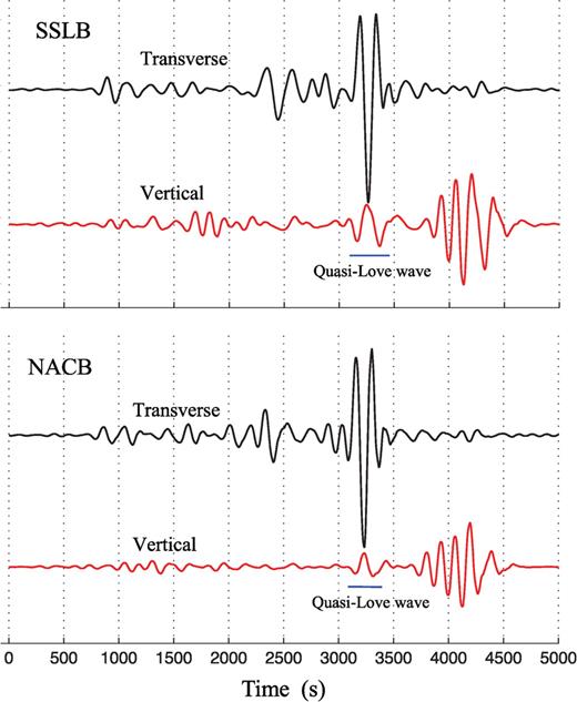
Vertical component seismograms recorded at SSLB and NACB showing obvious quasi-Love after the 2010 February 27 Chile earthquake. Waveforms shown are corrected for the instrument response and filtered between 2 and 8 mHz.
Observations of anisotropic coupling modes below 3.5 mHz remind us that we cannot ignore the possibility that the azimuthal anisotropic structures may be extend to the transition zone beneath Taiwan Island. Fig. 11 shows the energy distribution of coupled modes discussed in this paper. The maximum energy densities of modes 0S20 and 0S25 are concentrated to a depth range of about 400-650 km, just within the transition zone, but these of 0T20 and 0T25 are mainly concentrated to the upper mantle above the transition zone. To estimate the depth sensitivity ranges of coupled modes 0S25-0T25 and 0S20-0T21, we estimate their coupling sensitivity kernels according to PREM model and formula (1). In Fig. 12, the coupling kernels for coupled modes 0S25-0T25 and 0S20-0T21, governing Love wave interaction, show peak sensitivity to anisotropic VP and VS parameters B and E at the depth range about 400-650 km, but show no sensitivity to the isotropic VS parameter D. This result is consistent with the computation results of Beghein (2008) that S-T coupling shows peak sensitive to some elastic parameters describing azimuthal anisotropy at the depth range about 400-700 km. The strong S-T coupling observed at stations of BATS most likely arise from the presence of azimuthal anisotropy in the upper-mantle transition zone beneath Taiwan Island.
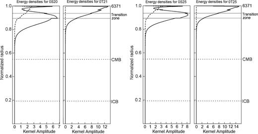
Energy densities of 0S20, 0T21 and 0S25, 0T25 for PREM model. Minos software package (Woodhouse 1988) is used in the calculations.
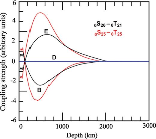
Depth sensitivity ranges of coupling pair 0S25-0T25 and 0S20-0T21. Dimensionless parameter D represents the isotropic velocity perturbations of S-wave, and B and E represents the azimuthal anisotropic velocity perturbations of P and S waves, respectively.
5, Interpretation and Discussion
Taiwan Island is the result of oblique collision between the Eurasian and the Philippine Sea plates. The convergence between two plates causes Taiwan moving at rate about 8.2 cm yr–1 in the direction of N54°W (Yu 1997). According to previous studies (e.g. Rau 2000; Teng 2000), the tectonic framework is complex at Taiwan Island. To the south of Taiwan, the Eurasian Plate is actively subducting eastward beneath the Luzon Arc, the oceanic lithosphere of the South China Sea and transitional lithosphere of the China continental slope sequentially going down into the Luzon subduction zone. Drastic collision commences in southern Taiwan, and the collision orogen grows to its maximum height in central Taiwan, as the continental lithosphere continues to subduct eastward. However, in northeastern Taiwan the subduction polarity has flipped, as the Philippine Sea Plate is underthrusting the Eurasian Plate. The orogen, no longer subjected to collision, is under the influence of lithospheric stretching and Ryukyu arc magmatism.
To form anisotropic structures in Earth's mid-mantle, lattice-preferred orientation (LPO) of anisotropic minerals or shape-preferred orientation (SPO) of secondary phases must be abundant and aligned into a strong petrofabric. LPO of α-phase is commonly accepted as the cause of strong anisotropy in the lithosphere (e.g. Savage 1999), so in general such an interpretation seems feasible for anisotropy in subducted slab. In contrast, SPO of hydrous phases or melt pockets requires a regional stress pattern (Chen & Brudzinski 2001). SPO of partial melt inclusions has been evoked to explained observed anisotropy in the lower mantle (Kendall 2000), but the presence of partial melt in the transition zone is not as likely (Boehler 1996). Focal mechanisms indicate that the subducted Eurasia slab is in downdip extension for depth of 150–230 km in southern Taiwan but switches to downdip compression at greater depths (Kao 2000). Therefore, SPO of hydrous phases may be responsible for deep anisotropy beneath southern Taiwan.
The breakoff of the east-dipping Eurasian slab beneath the Taiwan orogen may account for the anisotropy in the transition zone beneath northern–central Taiwan. According to the Taiwan plate motion model of Teng (2000), the breakoff of the subducted Eurasian slab first began in southern Ryukyu in the early Pliocene and has since propagated into northeast Taiwan, creating a mantle window for the north-dipping Philippine Sea Plate to fill in. Geological and geophysical observations at Taiwan Island in the past 20 yr are consistent with the notion that the Eurasian slab has broken off and sink into the deep mantle beneath northern Taiwan, and is in the process of breaking beneath central Taiwan (e.g. Crespi 1996; Rau 1996; Lee 1997; Kao 1998). Metastable phases such as olivine αphase, volatiles in the form of hydrous phases must be brought down to the mantle by subduction. As the breakoff of the Eurasian slab, a cold slab, descends into the mid-mantle and most of its olivine-polymorph remain in αphase, metastable olivine would make the leading edge of slab buoyant (e.g. Bina 1996; Marton 1999). However, this portion will never float above the 410-km discontinuity where warmer olivine of the ambient mantle is also in αphase. The transition zone holds subducted material and hinders slab penetration into the lower mantle. Thus, buoyancy of the slab is a self-limiting process confined to the transition zone (Chen & Brudzinski 2001). Northern–central Taiwan is a region where impounding of breakoff material is significant, favouring accumulation of metastable olivine or volatiles. Cold breakoff slab forms petrologic anomaly that is buoyant and stagnates in the transition zone beneath northern–central Taiwan, and can manifest itself through strong S–T coupling.
The S–T coupling caused by azimuthal anisotropy is strongest on the Rayleigh wave nodal lines and disappears at Rayleigh wave loop lines (Oda 2005), and it is significant at geometric nodes of spheroidal modes (Hu 2009). The data analysis in this report confirms that even with the existence of local azimuthal anisotropic structure near seismic stations, observable nSl–n′Tl′ coupling cannot be induced by the anisotropy when the stations are far from nodal lines of spheroidal mode of nSl. Small amplitude of spheroidal mode is a precondition for observing anisotropic coupling. It is therefore no surprise that sometimes the anisotropic coupling is unnotable at Taiwan Island after some other large earthquakes (see Table 1).
In summary, azimuthal anisotropy in the mid-mantle can cause notable long-period coupled modes at seismic stations near nodal lines of spheroidal harmonics, which provides an unignorable signal in analyzing of geodynamic structures. The details of the anisotropic coupling, being well worth a further study, can provide constraints on the results of anisotropy study by other methods.
Acknowledgments
We appreciate BATS, F-net and IRIS-DMC for their data being used in this study. The National Natural Sciences Foundation of China, under grants 41174022 and 41021003, supports this study.
References
