


Summary
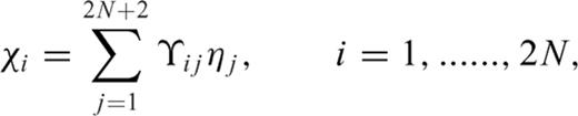
Crack models suitable to describe transcurrent faulting in the presence of a softer shallow layer are presented. We employ the asymptotic theory of generalized Cauchy kernel equations to study the singular behaviour of a strike-slip crack crossing the welded interface between two different media. If a planar crack cuts vertically across a material discontinuity, the dislocation density is bounded at the interface, but a stress drop discontinuity condition must be met, in which the stress drop is proportional to the local rigidity. Such a condition cannot be fulfilled in several cases. Two antiplane strain models are proposed to avoid this difficulty. In the first model (Fault bending model), the fault surface is affected by a sharp change of the dip angle at the intersection with the interface. An unbounded singularity in the dislocation density distribution (and in the stress field) appears at the interface and its dependence from model parameters is studied. A generalized stress drop condition is obtained which can be interpreted in terms of the interaction of the crack with the welded boundary condition. In the second model (Fault branching model), the crack is split into three interacting sections, with the lower section vertical and the other two sections inclined with respect to the vertical. In this case the order of the singularity at the interface remains undetermined. This result may be interpreted in terms of the further degree of freedom introduced by the presence of a second fracture in the upper layer. In the case of branching, two conditions are obtained for the stress drop on the three sections. According to both models, the generalized stress drop conditions may account for a stress drop ratio, between the soft layer and the hard basement, lower than the rigidity ratio.
1 Introduction
Surface maps of faults usually show complex geometrical patterns: fault bending and branching along the strike direction is the rule rather than the exception, suggesting a fractal distribution of faults (e.g. Shaw 1981; Aviles 1987; Okubo & Aki 1987). The irregular fault geometry is considered to be responsible for the generation and preservation of stress heterogeneities (e.g. Andrews 1989). These features are generally interpreted as the result of processes of near-surface segmentation. Many field observations support this interpretation: recent geological and geophysical studies of several stepover zones along the San Andreas Fault system in California reveal that the complex nature of the fault zone at the surface masks a much simpler geometry at depths (>5 km) associated with large earthquakes, as determined by accurately relocated hypocentres (Graymer 2007). In particular, gravity, magnetic and seismicity studies suggest that the Hayward and Calaveras faults in Northern California merge at 3-5 km depth (Ponce 2004); in the Parkfield region (Central California), the complexity shown by surface traces and the discordance of the location and geometry of the mainfault trace relative to the seismicity appears limited to the upper few kilometres (Simpson 2006). It is not a coincidence, probably, that in the fault region a sharp transition of seismic wave velocity is observed at comparable depth (Lin 2010).
Simple at depth extensional stepovers have been also proposed for the North Anatolian Fault section activated during the 1999 Ismit (Turkey) earthquake (Aochi & Madariaga 2003), for the Nojima-Rokko Fault system of the 1995 Kobe (Japan) earthquake (Wald 1996) and for the complex fault system associated with the 1992 Landers, California, earthquake (Felzer & Beroza 1999). In Fig. 1 the system of fractures is shown, which was left in the South Iceland Seismic Zone (SISZ) after the M6.6 earthquake of 2000 June 17. Lines of fractures parallel to the strike direction, but distant hundreds of metres from the fault trace, have been identified and clearly cannot be justified only in terms of the stress released by the vertically dipping main fault, well costrained by the distribution of aftershocks and by the fault plane solution (Stefánsson 2011). The post-seismic microearthquake activity is sharply confined below 3 km depth, so that the bending/branching point is inferred to be shallower and probably connected with major discontinuities in the velocity profile (Vogfjörd 2002; Antonioli 2006).
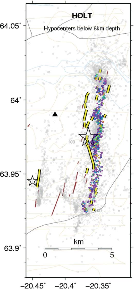
Aftershocks (dots) and pattern of surface fractures (double lines) in the SISZ earthquake of 2000 June 17 (Hjaltadóttir & Vogfjörd 2005).
When surface fractures appear laterally on one side of the deep fault strike, they can be ascribed to a bending process (Fig. 2a) while a branching process can be invoked when two or more parallel fractures are found on both sides (Fig. 2b).
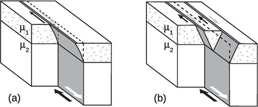
Schematic representation of a bending process (a) and a branching process (b). The fault sections are shown in grey, the slip is shown by the large arrows. Double lines denote surface fractures, the dashed line is the surface strike of the deep section.
Non-planar fault geometries have been investigated by many authors since geometrical complexities, such as bending (change of strike and/or dip), branching and stepovers, may play an important role in nucleation, propagation and termination processes of an earthquake rupture. The change in strike (bending process) of a strike-slip fault was studied by Duan & Oglesby (2005) to examine the long-term effects of a non-planar fault geometry. Kame (2003) considered the propagation of a mode-II rupture on a pre-existing branched fault to study the effects of pre-stress state and rupture velocity on dynamic branching. Also many experimental studies were performed to study the influence of bending and branching on shear ruptures (e.g. Rousseau & Rosakis 2003), with the purpose of simulating earthquake rupture processes. An important question is why and how such complexities originate since quasi-static crack solutions in a homogeneous medium show that an isolated model fault never bends if the fault extends in the direction of maximum shear traction beyond the tip. Kame & Yamashita (1999) showed that fault bending may take place even in a homogeneous medium if the rupture velocity approaches the shear wave speed, due to dynamic stresses deflecting the direction of maximum shear traction. Employing the same technique, Ando (2004) describe the interaction between fault segments, resulting in cohalescence or repulsion depending on their offset distance. Even if dynamic effects may produce fault bending in a homogeneous medium, non-planar fault geometries must be necessarily taken into account when the faulted medium is heterogeneous, as pointed out by Rybicki & Yamashita (2008), because the fault may bend abruptly at the interface between different media, where the orientation of principal stresses changes discontinuously. In particular, an explanation in terms of elastic heterogeneities allows preserving the fault bending geometry during several earthquake cycles.
The effects of crustal heterogeneities on transcurrent faulting processes have been investigated by many authors. A review of dislocation models in layered media is provided in a beautiful book by Segall (2010). A numerical code for solving point-dislocation problems in elastic and viscoelastic media is provided by Wang (2006). Rybicki (1971) studied the deformation field due to a strike-slip fault in a layered medium, showing that aftershock activity is affected by the residual stress field left after a major earthquake. Rybicki & Yamashita (1998) have shown that low-rigidity media may represent a barrier for fracture propagation in the case of faulting in vertically inhomogeneous media. Analogous results were obtained by Kame (2008) studying the quasi-static growth of strike-slip faults in presence of layered media and Hirano & Yamashita (2011) providing a convenient mathematical framework to analyse faults located along or across a material interface. The presence of a shallow soft layer was invoked by Belardinelli (2000) to interpret the complex pattern of surface fractures observed in the SISZ.
Dislocation models assume that the displacement discontinuity is assigned (and typically is piecewise constant) over the fault surface. On the contrary, crack models assume that the stress drop is assigned as a bounded function prescribed over the fault surface. The stress drop must be bounded because unbounded tractions cannot be sustained over a faulted surface. Due to the singular nature of the integral equation describing crack equilibrium, bounded tractions over the failure surface are generally accompanied by stress singularities beyond crack tips, even in a homogeneous medium. If a crack meets the welded interface between two different elastic media, a further singularity appears at the intersection (e.g. Erdogan 1973).
Bonafede (2002) have employed crack models to study theoretically the deformation and the stress fields induced by a planar strike-slip fault cutting the interface between different layers. A stress drop discontinuity condition was derived as a necessary condition that has considerable influence on the style of faulting in layered media. In fact many relevant geophysical cases are incompatible with the development of a planar fault and therefore complexities including fault bending, fault branching and the development of en echelon system of fractures must be involved in transcurrent fault processes within layered media. The aim of this work is to study fault bending and fault branching using the mathematical framework of crack models in 2-D antiplane configuration. This approach allows finding admissible solutions taking into account that singular stress values are unacceptable over the crack surface even if the dislocation density is found to be generally singular at the interface.
2 Preliminaries
Dislocation models are generally employed to model the deformation and stress fields after faulting events. The simplest dislocation model (hereafter termed ‘elementary dislocation’ accounts for a constant discontinuity Δu of the displacement field (Burgers vector), prescribed over a half-plane terminating at the dislocation line (e.g. Landau & Lifshitz 1967). It is well known that elementary dislocations face severe physical problems: the stress field in proximity of the dislocation line has a non-integrable singularity (of order -1) both within the faulted half-plane and beyond, the energy required to generate an elementary dislocation is infinite, continuity and impenetrability of matter are violated. If Δu is not constant and vanishes approaching the dislocation line, the order of singularity of the stress field changes.

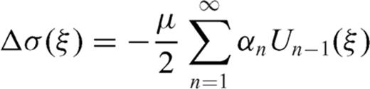
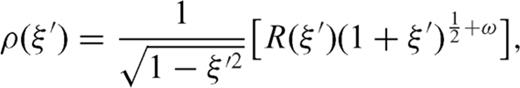
 . In order that finite values of Δσ are obtained over the crack surface -1 < ξ < 1, the dislocation density distribution ρ(ξ′) must possess a singularity of order
  close to crack tips (e.g. Muskhelishvili 1953):

 (with ξ= cosθ) are Chebyshev polynomials of the second kind.
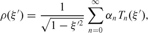
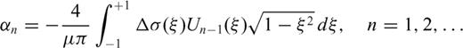
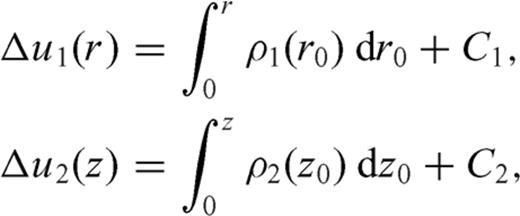
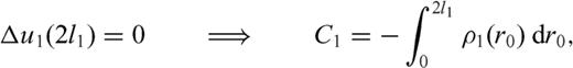
From eq. (2) it appears that the coefficient α0 is left undetermined by the integral equation, since the term n= 0 does not provide any stress release over the crack surface (the term n= 0 is solution of the homogeneous version of the integral eq. 1). In simple problems, α0 must vanish if we assume that the crack slip vanishes at both ends. Some dislocation problems however require that a crack may be open at one end: an example is provided by a crack opening at the free surface of a half-space (see case B1 in Bonafede & Rivalta 1999b) and in such a case a supplementary condition must be provided to fix α0, which may be obtained from the requirement that tractions on the free surface vanish at the intersection with the crack tip. More generally, one might conceive the problem in which one crack is split into two interacting sections: then both sections must be open at the merging point and each of the two dislocation distributions ρ1 and ρ2 will contain an undetermined coefficient for n= 0. Two supplementary conditions are then needed: one is simply provided by the request that slip is continuous passing from one section to the other, while the second can be obtained imposing that the singular traction produced by section 1 onto its own crack surface cancels with the contribution produced by section 2 and vice versa. Even if this case may seem only of academic interest, its solution is required to address the more complex problems in which two crack sections are embedded in different media with rigidity µ1 and µ2 (see e.g. Bonafede 2002) and/or are not coplanar, which is the target of this paper.
 ):
): 

3 Fault Bending Model
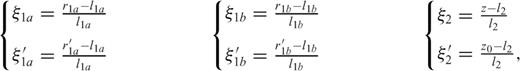
We consider an elastic half-space in z < 0 with rigidity µ1 welded to an elastic half-space in z > 0 with rigidity µ2. The origin of the reference system is placed at the intersection between the crack and the interface, with the z-axis pointing downwards. We consider an antiplane strain configuration in which the only non-vanishing component of the displacement field is uy(x, z), which is independent of the y-coordinate.
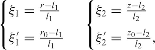
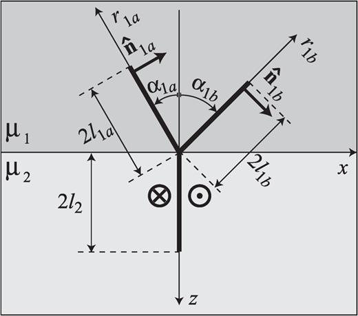
It is convenient to split the crack into two interacting sections, each embedded in one medium and both open at the interface. The section in the upper layer has length 2l1, it is inclined by an angle  with respect to the negative z-axis and its unit normal is
  The section embedded in the lower half-space is normal to the interface and its length is 2l2. A sketch of the model is presented in Fig. 3.
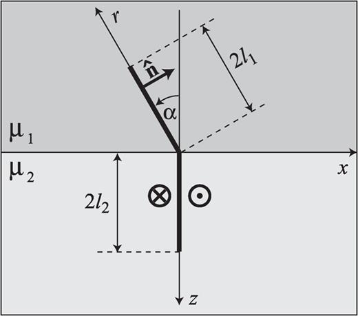
Bending model: the fault sections are shown as thick segments and the slip is normal to the plane of the figure.
- (i)
 are the tractions induced on section 1 due to crack slip on section 1 (I) and on section 2 (II), respectively;
 - (ii)
 are the stresses induced on section 2 due to crack slip on section 2 (II) and on section 1 (I), respectively.
 relative to a surface having
  as normal versor; we have
 and
and  are singular when r=r0 and z=z0,
  is singular only when r=z0= 0 and
  is singular only in z=r0= 0, so that integrals must be evaluated in the principle-value sense.
The integral kernels  , for an elementary screw dislocation of arbitrary dip embedded in the upper layer are given by Singh & Rani (1994), while the kernels
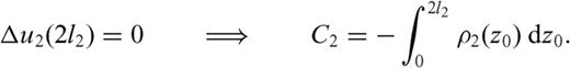
  can be obtained using the analytical solutions proper to a vertical screw dislocation (Bonafede 2002). Once the stress drops Δσ1, Δσ2 are assigned, the equilibrium equations become a system of coupled integral equations for the unknown functions ρ1, ρ2.


3.1 Supplementary conditions


 and
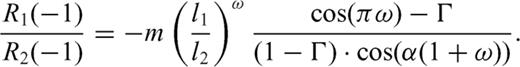
and  are regular functions [with R1(± 1), R2(± 1) ≠ 0]. With respect to the case of a planar fault, a singularity of order ω now appears at the interface and its value is dependent from model parameters α, m, as shown in Fig. 4, while the relative lengths of the two crack sections have no influence on its value [the ratio
  disappears in the derivation of eq. (A16)]. Once the inclination angle α is fixed, Fig. 4(a) shows that an increase of the rigidity contrast determines a significant increase of the singular degree ω only for m≲ 5. Instead, however we fix the rigidity contrast, the increase of α always determines a significant increase of ω, as shown in Fig. 4(b). We can also observe that the singularity degree ω is always greater than
  (see Fig. 4b), and this consideration will be useful in the next section to deploy a method of solution.
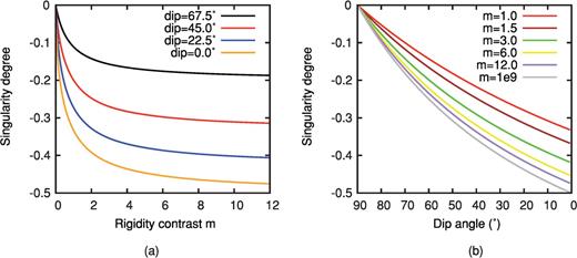
Dependence of the singularity degree ω from the rigidity contrast m=µ1/µ2 and the dip angle δ = 90° -α. Note that the dislocation density is bounded at the interface (ω= 0) only if the two crack sections are coplanar (vertical). The dislocation density must be singular at the bending point even if medium is homogeneous (m= 1).
 , it is easy to verify that
  .
.In the homogeneous case, ω takes lower absolute values with respect to the heterogeneous case (m > 1) since only two singular terms must be balanced on both crack sections. The third singular terms are only present if m≠ 1 (Γ≠ 0) and they describe how the rigidity contrast affects the stress release which each crack section produces on itself (second term on the right-hand side of eqs 13 and 14).
3.2 Method of solution
 in Jacobi polynomials
  , which are the orthogonal polynomials for the weight function
 , since we know that the singularity degree is always in the interval
  (as shown in Fig. 4b, Section 1.1); in this case
  can be expanded in a uniformly convergent series of Chebyshev polynomials even if the correct order of singularity of ρ(ξ′) near ξ=-1 cannot be reproduced when the series is truncated to a finite index. After these considerations, the dislocation distributions ρ1, ρ2 can be written as
 and
and  in the integral equations, the singular Cauchy kernels can be disposed of analytically.

 and integrating on the interval -1, 1 in the variable ξ1 we obtain
 and then integrate on the interval -1, +1 in the variable ξ2 we obtain
 and
and  are, respectively, the coefficients of the expansion of the stress drops Δσ1 and Δσ2 in Uk polynomials. If Δσ1 and Δσ2 are constants, then only
  and
and  differ from zero. The system of eqs (33) and (36) may yield a unique solution if we consider the supplementary conditions introduced in Section 3.1. If we introduce in (20) the expansions of ρ1 and ρ2 in Chebychev polynomials and we use the orthogonality relation between these polynomials
 and
and  coefficients can be obtained considering the ratio between ρ1 and ρ2 and letting t→-1
 , as expressed in eq. (23).
To provide an approximate solution to the crack problem, the infinite sums in (33) and (36) are truncated to a finite index N. More specifically, this means that in (33) and (36) we take
- (i)
Sij(k, n) = 0 for k > N- 1 ∧n > N;
- (ii)
 for k > N- 1.
 and
and 


3.3 Generalized stress drop condition

 , we obtain
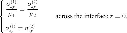

 and
and  must be continuous across the interface and the residual tractions acting on the fault sections are
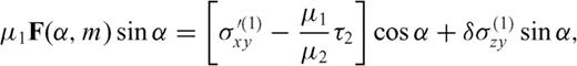
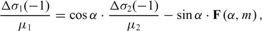
 is the zy-component of released stress at the bottom of the inclined fault section. The first term on the right-hand side vanishes due to the first condition (50) in the primed configuration, so that µ1F(α, m) can be always interpreted as
  at the intersection between the crack and the interface. Once µ1, µ2, α, Δσ1 and Δσ2 are fixed, the stress change
  is determined; alternatively, if
  is assigned, α is determined. For instance, in the limit case
  , we have
  ; vice versa, if
  , then
  . Since
  has no influence on the deep fault section, a configuration can be always conceived in which
  ; then F(α, m) = 0 and
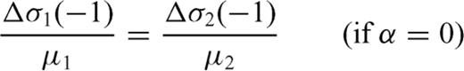
 : if the equality sign holds, then α= 0 (the fault crosses the interface without bending); if Δσ1= 0 (the initial stress in the upper layer equals the residual frictional level, as expected e.g. in an elasto-plastic medium with Mohr-Coulomb rheology), then
  and the upper layer unwelds from the deeper layer.
3.4 Numerical results
Following the previous analytic scheme, numerical computations have been performed assuming:
- (i)
ν1=ν2= 0.25 and µ2= 3µ1= 30 GPa,
- (ii)
2l1= 2l2= 8 km for the length of crack sections,
- (iii)
a stepwise constant stress drop profile with Δσ2= 3 MPa and
 .
.
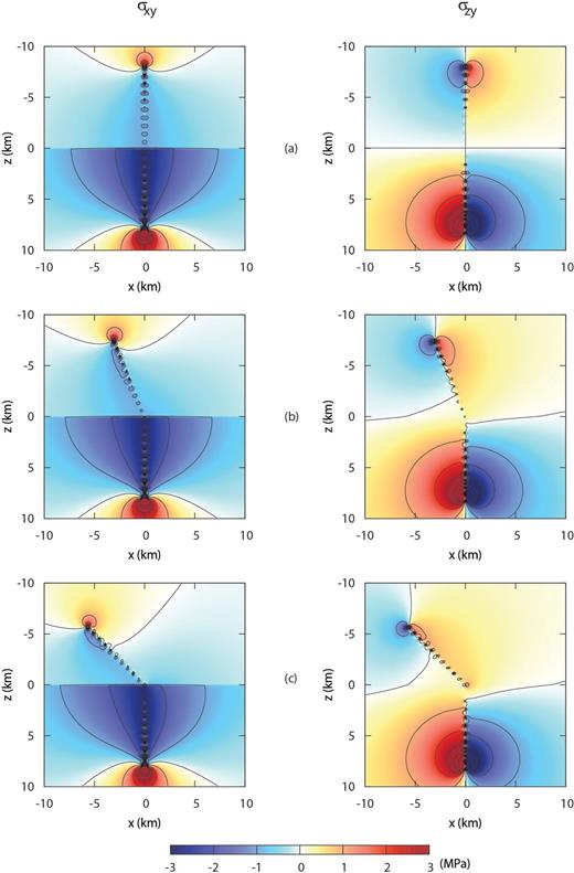
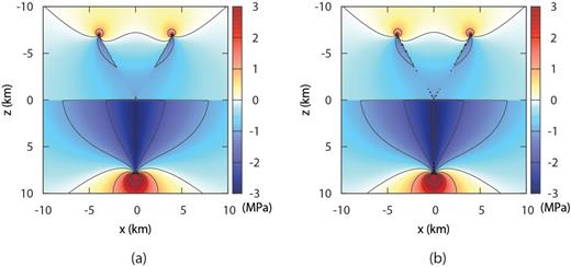
The non-vanishing stress components σxy and σzy induced by shear cracks corresponding cases
- 1
α= 0,
- 2
 ,
, - 3
 ,
,
are shown in Fig. 5. If we compare cases (2) and (3) with the case of a planar shear crack (Fig. 5a), we observe an asymmetric stress release with respect to the negative z-axis; the stress release is concentrated in the footwall block, while a minor release of σxy is observed in the hanging block, which is accordingly candidate to host new fractures.

Non-vanishing stress components σxy, σzy induced by shear crack with: (a) α= 0°, (b) α= 22.5°α and (c) α= 45°. A mild singularity is present (out of the crack surface), which can be barely appreciated only when α is large (insets in the lower panels).
From the asymptotic study we know that ρ1 and ρ2 are singular at ξ=-1 if α≠ 0 and this implies that also the stress components σxy and σzy are singular, but from Figs 5(a) and (b) we see that these singularities affect only a limited region around the bending point.
To check the accuracy of the approximate solution found, we show in Fig. 6 the stress components σxy, σzy computed according to the displacement discontinuity method (Crouch & Starfied 1983). This numerical technique does not involve a study of the singular nature (assuming that the order of singularity is equal to -1 at the ends of each boundary element) and provides accurate results only at distances from the fault much greater than the length of the dislocation elements. Therefore we can check the correctness of the results found employing the crack model. The comparison of stress maps shown in Figs 5 and 6 is satisfactory (away from the fault surface, of course), confirming the crack model approach. It must be stressed that the boundary element method cannot provide indications on fault bending, because singular stress values are always obtained over the fault surface, which must be assumed known a priori, while the crack model provides such indications since singular tractions are not admissible over the crack surface and the bending angle α is strictly linked to the stress drop discontinuity condition.
Non-vanishing stress components σxy, σzy computed according to the displacement discontinuity method: (a) α= 0°, (b) α= 22.5° and (c) α= 45°.
4 Fault Branching Model
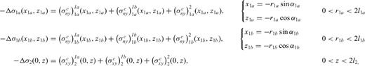
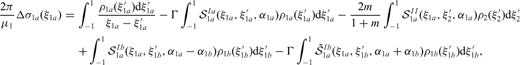
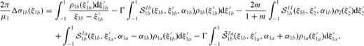
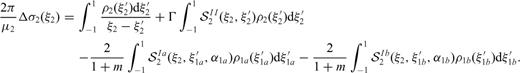
The bending crack model is clearly symmetric if we change the sign of the bending angle α. We have already noted that more stress is released in the footwall block than in the hanging block and this leads to envisage that the hanging block will host an inclined fault section accompanying future deep events. Therefore we consider in the following a branching crack model in which the crack is split into three interacting sections, all open at the interface, but with sections 1a and 1b embedded in the upper layer and section 2 embedded in the lower half-space (Fig. 7). The sections 1a and 1b have length 2l1a and 2l1b, respectively; both sections are inclined with respect to the negative z-axis ( and
and  represents the normal versor of section 1a, while
  is the normal versor of section 1b. As in the previous model, section 2 is normal to the interface, with length 2l2.
Branching model: fault sections are shown as thick lines. Slip is normal to the plane of the figure.
- (i)
 are the tractions induced on section 1a due to crack slip on section 1a (Ia) and 1b (Ib), respectively, while
  is the traction induced on section 1a due to crack slip on section 2 (II);
 - (ii)
 are the tractions induced on section 1b due to crack slip on section 1a (Ia) and 1b (Ib), respectively, while
  is the traction induced on section 1b due to crack slip on section 2 (II);
 - (iii)
 is the stress induced on section 2 due to crack slip on section 2 (II), while
  are the stresses induced on section 2 due to crack slip on section 1a (Ia) and on section 1b (Ib), respectively.
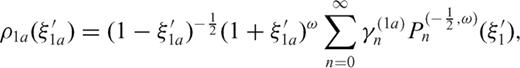
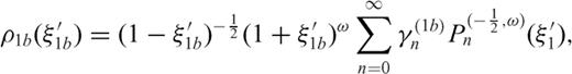
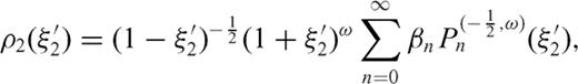
 , a distribution ρ1b with dislocation lines in the interval
  and a distribution ρ2 with dislocation lines in the interval 0 < z0 < 2l2; the dislocation density distribution ρ is so split into three subdomains
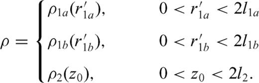


 and
and  are equal to the integral kernels
  and
and  in eqs. (16) and (17) if we put α=α1a in case of section 1a and α=α1b in case of section 1b. Instead
  are generalized Cauchy kernels that describe the stress drop induced on section 1a due to slip on section 1b.

 and
and  describe the stress drop induced on section 1b due to slip on section 1a and have the same expressions of the integral kernels
  and
and  if we exchange the suffix 1a and 1b in the eqs (60) and (61).
In eq. (59), the singular kernel  has been already introduced in eq. (18), while
  and
and  are equal to the integral kernel
  presented in eq. (19) if we put α=α1a and α=α1b, respectively.
4.1 Method of solution
 and b1a=b1b=b2=ω are necessary conditions to have finite stress release over each crack section (all the three dislocation densities must have the same singularity degree at the interface). To evaluate ω, the condition is imposed that the traction is bounded over the crack surface at the intersection: accordingly, compensation of singular terms provided by each crack section must be imposed and this condition provides three homogeneous linear equations for R1a(-1), R1b(-1) and R2(-1), with coefficients aij depending on ω and on α1a, α1b, m, l1a, l1b and l2.
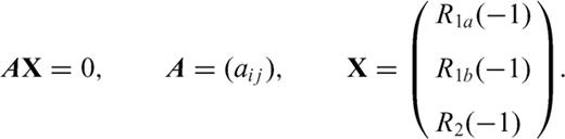
 ), so that no condition is extracted for ω. Therefore, any value of ω within the allowable interval) - 1, 0] can be considered as acceptable and only the ratios R1a(-1)/R2(-1), R1b(-1)/R2(-1) can be evaluated
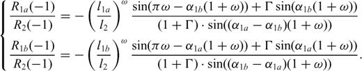
- (i)
the angles α1a, α1b must be different (α1a≠ α1b) in order that the denominators in (63) do not vanish,
- (ii)
the values ω=ω1a and ω=ω1b for which a single fracture develops in the upper medium with angle α=α1a and α=α1b, respectively, must be excluded since R1a(-1), R1b(-1) must not vanish. In fact the numerators in (63) reproduce the second factor in eq. (A17), the condition that identifies the singular degree of the dislocation density at ξ=-1 in presence of a single fracture in the upper medium (fault bending model).
To obtain information about the singular nature of the dislocation density at the interface, we are forced to adopt a different approach. We choose to use the displacement discontinuity method, since this numerical technique can be applied without any previous knowledge about the singular nature at crack tips. To apply this method, we need to know which are the stress drops to assign over the crack sections and therefore we must compare, as done for the fault bending model, the finite contributes to stress drop at the branching point.
4.1.1 Stress drop conditions


 has this form


 undefined.
 as the zy-component of released stress at the bottom of the two inclined fault sections. If we assume that only σxy is released then the stress conditions derived reduce to
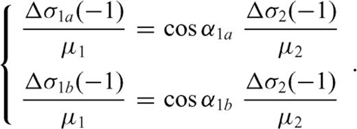
Once the stress drop conditions have been derived, then we can apply the displacement discontinuity method. If we consider Fig. 8(a), no singularity seems to be present at the crack tip ξ=-1 (the origin of the reference system) and if we perform a more detailed calculation with higher resolution in proximity of the interface (Fig. 8b) this conclusion is confirmed. Thus, there is no need to assume a singularity for ρ at the branching point and in the following we will consider ω= 0.
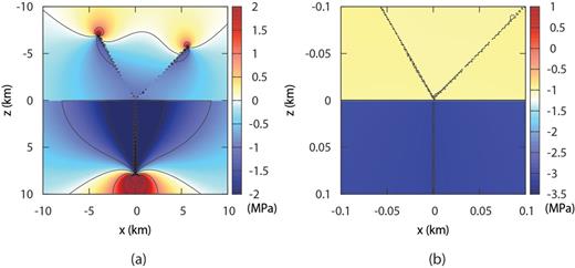
Stress component σxy computed according to the displacement discontinuity method (with α1a= 30°, α1b=-45°): (a) in a region of 20 km x 20 km (with N= 20 boundary elements for each crack section), (b) in a region of 200 m x 200 m (in this case a non-uniform distribution of boundary elements was used, with higher density close the origin).
In this case the form of the singular factors suggests expanding R(ξ′) in Jacobi polynomials  , which are orthogonal if the weight function w(ξ′) = (1 -ξ′)-1/2 is employed and the relations (64)-(66) reduce to


Each crack section is open at the interface, therefore we must supply three supplementary conditions in order that the problem may yield a unique solution.
4.2 Supplementary conditions


 are ultraspherical polynomials that, if
  , reproduce Legendre polynomials Pk(t). The normalized dislocation density
  can then be rewritten in the following form:
 coefficients differ from βk in eq. (75c) by a factor of
  . The presence of the singular factor t2-1 in eq. (78) should be of no concern, since ρ2 always appears through integrals when observable quantities are considered and
  . For instance, if we compute the displacement discontinuity Δu2, we obtain
 can be written through expansions similar to (78).

 and between

4.3 Approximate solution: truncated problem


- (i)
substitution of (78), (81) and (82) in the integral equations and
- (ii)use of the integral relationvalid for Jacobi polynomials to perform analytically the first integration, where Qk(t) are Legendre function of the second type (e.g. Gradshteyn & Ryzhik 1965);(92)

- (iii)
each equation must be multiplied by
 and then integrated on the interval [-1, 1] in the variable ξ to obtain Sij(k, n) coefficients.
 and
and  are the coefficients of the expansion in Uk polynomials of the stress drops Δσ1a, Δσ1b and Δσ2, respectively. If Δσ1a, Δσ1b and Δσ2 are constants then
  and
and  are the only coefficients different from zero.
To provide an approximate solution to the crack problem, the infinite sums in (87)-(91) are truncated to a finite index N. More specifically, this means that in (89)- (91) we take
- (i)
Sij(k, n) = 0 for k > N- 1 ∧n > N and
- (ii)
 for k > N- 1.


4.4 Numerical results
The computations have been performed assuming:
- (i)
ν1=ν2= 0.25 and µ2= 3µ1= 30 GPa;
- (ii)
2l1= 2l2= 8 km for the length of crack sections;
- (iii)
a stepwise constant stress drop profile with Δσ2= 3 MPa and
- 1
 ,
, - 2

- 1
In Fig. 9, we show the stress drop and the crack slip corresponding to the following three cases:
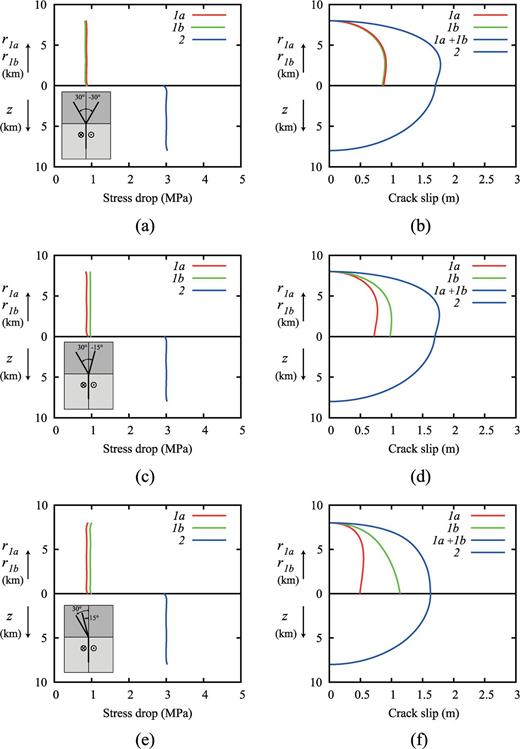
Stress drop and crack slip on crack sections in three different geometrical configurations: (a,b) α1a= 30°, α1b=-30°, (c,d) α1a= 30°, α1b=-15°, (e,f) α1a= 30°, α1b= 15°.
(I)  ;
;
(II)  ;
;
(III)  .
.
The approximate solutions reproduce with great accuracy the stress drop profile if the infinite sums in (78), (81) and (82) are truncated to N= 10. In case I (Fig. 9a) the stress drop over crack section 1a and over crack section 1b have the same value and furthermore (Figs 10b and c) are identical since the stress drop on section 1b have the same value in both cases.
Stress component σxy induced by a fault branching process (with α1a= 30°, α1b=-30°) calculated by the method of solution proposed in Section 4 (a) and, for comparison, with a boundary element approach (b) in which 20 elements for each sections have been considered.
As expected, the crack slip on the inclined sections has the same profile when the sections are symmetric with respect to the negative z-axis (Fig. 9b), while in cases II and III the crack slip is significantly affected by the relative position of sections 1a and 1b (Figs 9d and f). First, we can note that the crack slip is split between section 1a and section 1b so that greater slip is observed on the less inclined section, since the other section feels more the higher rigidity of the lower medium (Fig. 9d). If both sections are in the same quadrant (Fig. 9e), the effect is amplified so that the crack slip has very different trends on section 1a and on section 1b.
To evaluate the accuracy of the approximate solution found, we show in Fig. 10 the stress component σxy computed according to the displacement discontinuity method. The comparison is satisfactory since the stress map obtained with the boundary element approach is reproduced with great accuracy apart from the very proximity to the crack surface.
Observing the stress maps corresponding to cases I-III (Fig. 11), we note that when the inclined sections are in opposite quadrants, case I (Figs 11a and b) and case II (Figs 11c and d), the release of the stress component σxy affects a wider region, while in case III (Figs 11e and f) the pattern of stress release is similar to that obtained in the case of a single inclined section, where no significant stress release is observed in the opposite quadrant. Further we can observe that the presence of two inclined sections provides a very variable pattern for the stress component σzy, since this component changes sign across each crack section (Figs 11b, d and f).
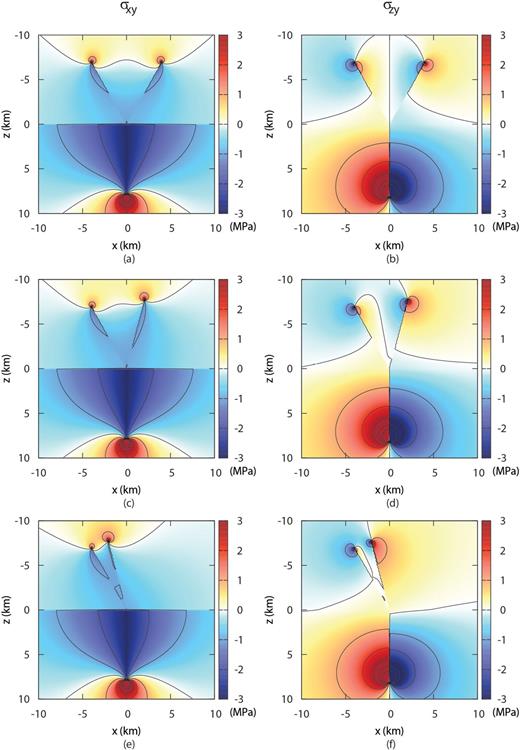
Non-vanishing stress components σxy, σzy induced by branching shear cracks with: (a,b) α1a= 30°, α1b=-30°, (c,d) α1a= 30°, α1b=-15°, (e,f) α1a= 30°, α1b= 15°.
The method of solution proposed involves the expansion of the dislocation density in Legendre polynomials since we have assumed ω= 0. The asymptotic study shows that the singularity degree can assume all the values in the interval] -1, 0]. Therefore a solution can be derived considering another value for ω and in Fig. 12 we show the stress drop computed according to the expansion of the dislocation density in Chebyshev polynomials, the method used to obtain numerical solutions for the fault bending model. As expected, this method of solution has a slower convergence, since now for N= 10 (Fig. 12a) the stress drop is very variable and even increasing the order of truncation to N= 100 (Fig. 12b) the accuracy decreases approaching the interface.
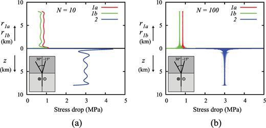
Stress drop on crack sections computed according to the expansion of the dislocation density in Chebyshev polynomials with truncation order N = 10 (a) and N = 100 (b).
5 Conclusions
We have presented two models of non-planar cracks cutting across a rigidity discontinuity, which may be suitable to describe strike-slip faulting in the presence of a shallow soft layer. If we consider the fault bending model, a singularity appears in the dislocation density at the bending point. An asymptotic study shows that the dislocation density has an infinite singularity ˜rω at the interface with  , depending on the dip angle δ = 90°-α of the upper crack section and on the rigidity contrast m. Once this singularity is properly accounted for, crack equilibrium requires that the stress drop values on either sides of the interface must satisfy eq. (51) to match the welded boundary conditions. Then, if the stress drop is assigned over both faults sections (according to fault rheology), a vertically dipping fault can cross the interface if the upper section is suitably inclined.
Considering the fault branching model, the study of the asymptotic behaviour leaves the singular degree of the dislocation density undetermined, with ω∈] -1, 0]. This indeterminacy has only a mathematical character and it can be interpreted in terms of a further degree of freedom introduced by the presence of the third crack surface. From a physical point of view, the simplest explanation is that no singularity is required at the interface and this guess is supported by the numerical results obtained employing the boundary element method. The stress drop on the three fault sections must satisfy two generalized conditions (67) and (68).
Large rigidity contrasts are typically found in the upper crust and the driving stress of strike-slip faults is strongly discontinuous across such layer interfaces. According to the previous models, we may assess that the presence of crustal layering calls for the formation of geometrical complexities in transcurrent fault regions.
Several field observations regarding the complex pattern of surface fractures connected with major strike-slip earthquakes may be explained in terms of such a mechanism. For instance, if we consider the case of the Ms= 6.6 earthquake of 2000 June 17 in Iceland (Fig. 1), the aftershock activity (dots) shows very well the NS orientation of the vertical main fault, confirming the fault plane solution, while lines of surface fractures (double lines) are observed laterally shifted up to ˜1 km from the deep fault strike.
Considering the fault geometry, since major rigidity discontinuities in the SISZ are found at 3 km and 1.5 km (Antonioli 2006), α can be inferred to be α˜18° or α˜ 30°, respectively, and the stress drop on the shallow section is negligible with respect to the deep section, suggesting that faulting propagated passively to the surface, as suggested also by the lack of aftershocks in the shallower 3 km (Stefànsson 2011). Similar considerations can be proposed also for the San Andreas Fault sections mentioned in the Introduction.
In the bending model, the inclination of the upper section determines an asymmetric stress release with respect to the negative z-axis, therefore the region with minor release is candidate to host new fractures. The stress singularity which is present close to the bending point (see insets in Fig. 5c) may be responsible for the localized microearthquake activity along the slip direction detected on strike-slip faults (e.g. Rubin 1999).
If the generalized stress drop condition (51) imposes low values of the inclination angle, it is reasonable to expect that only a bending process takes place since the singularity degree at the bending point is low (Fig. 3b). Instead, when very low stress drop values are applied on the upper section, the stress drop condition requires higher values for α and the higher values of the singularity should favour a branching process. In Fig. 1 we can observe that multiple surface fractures appear when their distance from the deep fault strike increases.
A limit case of fault branching takes place when a low level of the driving stress ( ) in the upper layer does not allow the propagation of the main fracture across the interface and the σzy stress component in excess of the frictional threshold is released; then the unwelding of the interface takes place
  . In Ferrari & Bonafede (2011) a parametric study of this process was performed employing a boundary element method in a layered medium bounded by a free surface to study the stress redistribution following the unwelding of near surface layers.
It must be mentioned that the models presented in this paper apply to a strictly antiplane strain configuration, assuming laterally uniform properties within each layer. Even in this framework, complexities of fault regions might be generated according to other mechanisms, such as dynamic effects mentioned in the Introduction, the presence of pre-existent weakness planes or strength heterogeneities of shallow layers. Finally, the study of stepover zones, where a planar fault section bifurcates into two separate sections near the surface, requires intrinsically 3-D fault models and cannot be addressed employing the present semi-analytic asymptotic approach.
Acknowledgments
This paper originates from several discussions with our partners in the framework of the UE project PREPARED, focusing on the SISZ (FP5RTD). We thank Eleonora Rivalta and an anonymous reviewer for constructive criticism on a previous version of this paper.
Appendices
Appendix A: Asymptothic Study
 or
or  .
.

A1 Singularities of ρ at crack tips

 and
and  are functions whose behaviour is similar to that of Φ0(ς).
A2 Singularity at ξ = 1
 and letting → 1, we find
 and considering the limit ξ→ 1, we obtain
A3 Singularity at the interface
 and letting ξ-1
 and considering the limit ξ→1,


Appendix B: Stress Drop Condition

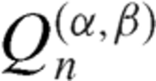 are Jacobi functions of second type that admit this representation
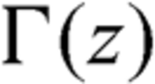 represent the gamma function while F(a, b; c; x) is the hypergeometric function
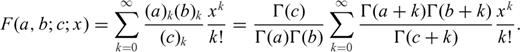


References
