


Summary
We present a series of 1-D shear velocity models for the Sumatran Forearc and Arc derived from Rayleigh wave group dispersion in noise correlation functions from vertical and pressure records from an onshore–offshore seismic deployment. The 1-D models represent the crustal structure of the downgoing Indian Plate, the accretionary prism and the arc. There is a progression in shear velocity across the forearc to the arc associated with thickening of the accretionary prism and the development of an arc crust. The velocity structure inferred for the upper 20 km based on path averages between stations on the accretionary prism has velocities consistent with a thick sediment package in agreement with estimates of depth to the plate boundary determined from active source experiments. We also find low Indian Plate shear velocities, <4 km s-’1 to 25 km depth beneath our station locations on the downgoing plate. These low seismic velocities are consistent with at least 14–24 per cent serpentinization of the oceanic crust and upper mantle of the downgoing plate. This high degree of serpentinization, may weaken the plate interface and explain the segmentation observed in the great Sumatran thrust earthquakes if the serpentinization is localized. The success of this study suggests that future onshore–offshore seismic deployments will be able to utilize this method.
1 Introduction
The Sumatran subduction system has produced three of the largest megathrust earthquakes in the past decade along different segments, the Andaman 2004 December 26 Mw 9.1–9.3 event, the Nias, Mw 8.7 2005 March 28 (Ammon et al. 2005; Lay et al. 2005; Konca et al. 2007) and the 2007 September 12, Benkulu Mw 8.5 events (Konca et al. 2008). These great earthquakes have ruptured most of the segments of the fault that have produced earthquakes of similar magnitude over the past 300 years, except one remaining segment of the fault, centred on Siberut Island. This segment produced an earthquake of Mw > 8.7–8.9 in 1797 but has not ruptured since (Chlieh et al. 2008). It now has a total slip deficit equivalent to an Mw 8.8 event (Sieh et al. 2008). The segment of the fault appears to be kinematically coupled to the downgoing plate based on uplift rates from geodetic and coral banding data, but is adjacent to an uncoupled region to the north near the Batu Islands (Chlieh et al. 2008). The weak coupling beneath the Batu Islands might be due to the subduction of the Investigator Fracture zone (Chlieh et al. 2008). In order to assess the potential hazard through studying the patterns of seismicity (Lange et al. 2010) and imaging the upper plate structure (Dean et al. 2010), the United Kingdom′s Natural Environment Research Council′s Sumatra Consortium project deployed short period ocean bottom seismometers (Minshull et al. 2005) equipped with differential pressure gauges (DPGs) for 10 months in conjunction with land deployments in the forearc between Nias and Siberut Islands (Henstock et al. 2010; Fig. 1).
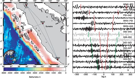
(A) Map of the region showing seafloor bathymetry, station locations (red triangles) and station-to-station paths presented in this study (grey lines connecting stations). Investigator fracture zone (IFZ) and nearby islands are labelled on the map. Inset map shows location of study area on the globe as a yellow star. (B) NCF for selecting station-to-station paths presented in this study (black) and results for shallow water stations 40 and 48 (grey) which did not produce usable results. Positive lags correspond to waves travelling from the first station to the second station, while negative lags correspond to waves travelling in the reverse direction. Red markers are predicted 3.5 km s-’1 traveltimes, green markers indicate 1.0 km s-’1 traveltimes.
Variations in the elastic properties of the materials along and across a fault segment can alter the effective normal stress on a fault to inhibit or initiate earthquake rupture either directly or through poroelastic effects (Rudnicki & Rice 2006). In addition, shear modulus is important for estimating displacement on a fault from seismic moment (Kanamori 1977). In remote inhospitable regions such as the seafloor, these properties are often not well known. The ocean bottom seismometer deployment provides a unique opportunity to examine the crustal shear velocity structure of the downgoing slab, as well as the accretionary prism using passive seismic techniques.
In this paper, our goal is to constrain the crustal structure of the Sumatran forearc in order to place better constraints on the physical properties of the upper part of the seismogenic zone. We use the DPG data, along with GEOFON network seismic stations to estimate the crustal shear velocity structure using short period Rayleigh wave group dispersion estimated from seismic noise correlation functions (NCFs; Shapiro & Campillo 2004; Sabra et al. 2005). While this technique has been successfully applied to ocean bottom data in the deep ocean (Harmon et al. 2007; Yao et al. 2011), across ocean basins it has only been shown that this method works at the longest periods (>70 s; Lin et al. 2006; Schimmel et al. 2011). Therefore, we also evaluate the effectiveness of DPGs for onshore–offshore noise correlation for future deployments.
2 Data and methods
We use 200 d of continuous ocean bottom DPG records from nine stations collected during the 10-month ocean bottom seismic deployment from 2008 April to 2009 February and vertical component data from land stations PSI operated by the Pacific21 network and stations BKNI (Bangkinang, Sumatra), MNAI (Manna, Sumatra), operated by the GEOFON network. Station locations are shown in Fig. 1. Instrument responses were removed from the land station data, converting the data to velocity traces and all data were down sampled to 1 Hz.
Prior to cross correlation, we normalize each seismogram with its envelope after Harmon et al. (2010), which is similar to the approach of Bensen et al. (2007). The data for each day were zero padded and Fourier transformed, spectrally whitened by amplitude normalization and cross-correlated (Bensen et al. 2007). The daily correlations for each station-to-station pair were stacked to generate the NCF. For our analyses, we use the symmetric component of the NCF.
We use spectrograms to estimate Rayleigh wave group velocity dispersion in the NCF (Figs 2 and 3). Using a sliding 60 s Hanning window (∼2× longer than the longest period of interest, 28 s), with a 1 s time step, we estimate the power through the NCF through time. Group velocities at each period of interest were then selected based on the maximum of the power. The data were in general noisy, therefore we chose group velocities only if the maximum was a factor of 10 or greater than the average background, that is, a signal-to-noise ratio (SNR) >10 in power. There are also numerous arrivals visible in the spectrogram at both super- and subsurface wave velocities, so we limited our picks to be between 0.50 and 4.50 km s-’1. Error in the group velocity pick is scaled to the width of region within 99 per cent of the maximum value at a given period (∼1 dB fall-off), which gives reasonable error ranges of 0.01–0.50 km s-’1.
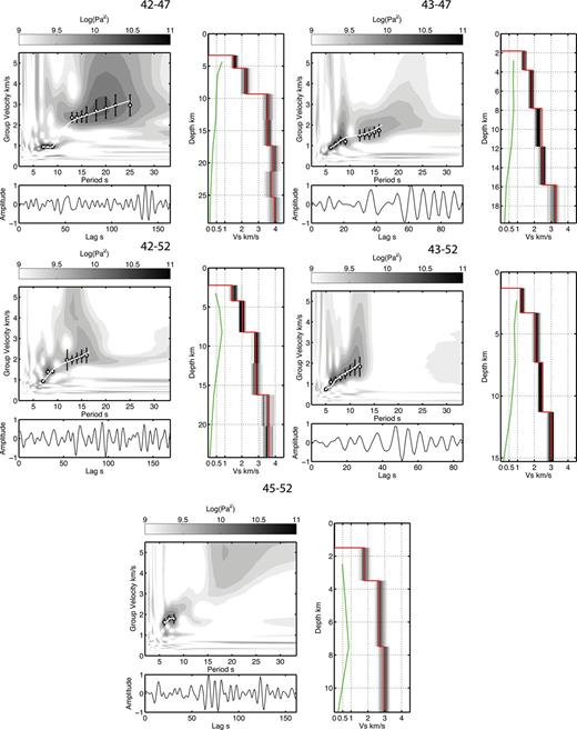
Offshore station-to-station path symmetric NCFs, spectrogram plots and shear velocity models. Each path is labelled above its respective plot group. NCFs are plotted beneath the corresponding spectrograms. Our picks for group velocity are plotted in each spectrogram (white circles), with the corresponding predicted group dispersion curve (white line) for the corresponding shear velocity plotted to the right-hand side (red line). Darker gray shading indicates higher probability density of acceptable shear velocity models. The green line in the shear velocity model indicates the diagonal elements of the resolution matrix corresponding to the different layers; models are only plotted to the deepest resolved model parameter (R > 0.1).
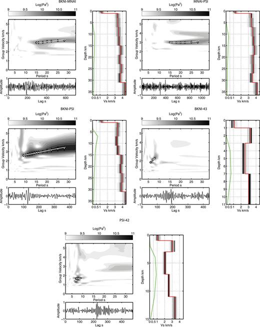
Onshore and onshore–offshore station-to-station path symmetric NCFs, spectrogram plots and shear velocity models. See Fig. 2 for format description.

We calculate the group velocity sensitivity kernels with respect to shear velocity using DISPER80 (Saito 1988). We use a starting model which has a generic crustal structure loosely based on the CRUST2.0 crustal model (Bassin et al. 2000) with a mantle structure taken from PREM (Dziewonski & Anderson 1981). We use up to six iterations in the inversion and an a priori model error of 0.5 km s-’1 to get the models to converge from our generic starting model. We use a model parametrization (2–5 km block size at 0–40 km depth) that produces a resolved minimum structure model while also allowing for the known rapid variation in shear velocity at shallow depths on the seafloor. The formal resolution matrix from eq. (1) is given by: R= (GTC-’1nnG+C-’1mm)-’1GTC-’1nnG, resolution shown here is the diagonal components of R corresponding to each model parameter. The formal resolution provides information about the independence of the model parameters and indications of trade-off with other model parameters. A formal resolution of 1 indicates a perfectly resolved model parameter, with no trade-offs.
To explore the range of possible models, we performed a Monte Carlo simulation to generate a probability density function of acceptable models. We randomly perturb our best-fitting velocity structure 1000 times and estimate the goodness of fit for each new velocity model. If the predicted group velocity is within error of the observations, the model is deemed acceptable. We then bin the acceptable velocity models with depth (same as our model parametrization) and velocity (0.10 km s-’1 bins) to create probability density function at each depth. We present this as the likely range of possible models and to determine if there are alternate families of acceptable models. Although these models fit the data, they are not smooth and therefore geologically unlikely. So we prefer our best-fitting models to these alternatives. We also present formal uncertainty from the inversion, but we note that this uncertainty under predicts the range of acceptable models.
Group dispersion is very sensitive to water depth, so we estimate the average water depth for each station-to-station path using shipboard swath bathymetry and satellite derived seafloor topography (Smith & Sandwell 1997). We fix the water depth in the model and set the water shear velocity to zero and compressional velocity to 1.5 km s-’1. For onshore paths, we use a generic shallow crustal velocity model based on the CRUST2.0 crustal model (Bassin et al. 2000) for Sumatra.
Out of the 66 possible station-to-station NCFs, we have confidence in six path averaged shear velocity models. We only selected NCFs that have good SNRs and clear wideband (to >15 s period) dispersion. This number was small because the SNR, defined by power spectral ratio, was small in general, with even our best NCFs only having SNR slightly greater than 10. In addition, the spectrograms (Figs 2 and 3), show multiple arrivals and heterogeneous distribution of coherent energy propagating across the array, evidenced by the variable frequency content of the NCFs. Some of these effects can be explained by the presence of the water column above the instruments and only using the pressure record. We discuss this in detail in Section 4.1.
3 Results
We divide our data into two groups, offshore, submarine NCF and onshore/onshore–offshore NCF. Examples of the NCF, spectrograms and shear velocity inversions are shown for offshore station-to-station paths in Fig. 2 and onshore–offshore and onshore station-to-station paths in Fig. 3. We present these path averages in this grouping to highlight the differences in frequency content and group velocity. Although we show results for the symmetric component dispersion of the NCF, measurements of dispersion on the positive and negative lags produced dispersion estimates within error for station-to-station NCF with good SNR. For each NCF, we also show the shear velocity model corresponding to the observed group dispersion, to depths that have a formal resolution from the diagonals of the resolution matrix of our damped iterative least-squares inversion of >0.1 (shown as the green line adjacent to the shear velocity scale is 0–1).
In the submarine paths, the clearest dispersion can be observed for the NCF for the path 42-to-47, with energy observed between 6 and 25 s period. In the spectrogram, we observe an Airy phase (flat dispersion) between 6 and 9 s period with velocities ranging from 0.93 to 0.95 km s-’1 due to the >3-km-thick water layer. At periods greater than 10 s, the group velocity jumps up to 2.37–2.83 km s-’1. The NCFs from 43-to-47, 42–52 and 43–52 exhibit energy in the 5–16 s period range, with low group velocities, ranging from 0.91 to 2.00 km s-’1. The NCF for 45–52 exhibits significant energy between 6 and 8 s, with a mean group velocity of 1.74 km s-’1.
The land station-to-station paths have significant energy at periods greater than 15 s in the case of BKNI-to-MNAI and MNAI–PSI and energy above 8 s period for BKNI–PSI. The group velocities for these three station-to-station paths is consistent, within 2 per cent of each other from 15 to 20 s period with a mean of ∼2.98 km s-’1.
In contrast, the onshore–offshore paths (BKNI–43 and PSI–42) have energy between 6 and 9 s period, within the secondary microseism band. The velocities in this range vary, with PSI–42 path having a lower average group velocity of 1.69 km s-’1 in this period range compared to 2.08 km s-’1 for BKNI–43. This may reflect the greater water depth at station 42.
Our Monte Carlo probability density functions generally show distributions centred on our best-fit preferred models for both the land and deep-water paths. For example, 42–47 shows a distribution that is centred beneath the best-fitting model. Other path average dispersion curves permit other families of models evidenced by peaks in the distributions away from our best-fitting models. Specifically, 42–52 shows that at depth below 12 km, a lower velocity model than our best-fitting model is also acceptable. Similarly, MNAI–PSI shows there may be multiple families of models, however the range of these models from 5 to 25 km depth, are generally consistent structures with the other land station paths.
We compare the shear velocity models in Fig. 4 for NCFs from 42–47 (cyan), 42–52 (red), 43–47 (red), BKNI–MNAI (black), BKNI–PSI (black), MNAI–PSI (black), which had resolution to >15 km depth. We find the offshore station-to-station paths have significantly lower shear velocity in the upper 8 km, with values ranging from 1.29 to 2.52 km s-’1 for the NCFs from 42–47, 42–52, 43–47 and 43–52 compared to the land stations pairs which ranged from 3.40 to 3.60 km s-’1 (ignoring the unresolved shallowest layer). In the 10–25-km depth range, the shear velocity for the deepest average water depth path, 42–47 increases into the range of the land stations, with a velocity of 3.53–3.98 km s-’1. From 8–15-km depth range 42–52, 43–47 and 42–52 are still significantly slower than the land stations and 42–47, with values of 2.33–3.04 km s-’1. These differences are well resolved based on formal resolution values (>0.4) in this depth range for the offshore NCFs. At greater depth, the shear velocity model for 42–52, 43–47 and 42–52 increase to 3.23–3.96 km s-’1, within error of the other station-to-station pairs for that depth. At >25-km depth the shear velocity model for path 42–47 increases to 3.94 km s-’1.
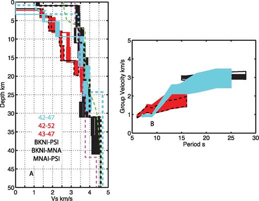
(A) Shear velocity comparison for the six best-resolved station-to-station paths. Models are colour-coded in the legend (red fill with black dashed indicates 43–47). Cyan dashed line indicates CRUST2.0 model for -’1°S, 98°E (oceanic path), black dashed is the CRUST2.0 model for 0° N, 100.5° E (arc path), green dashed is the 1-D shear velocity model of Collings et al. (2012), and purple dashed is the 1-D shear velocity model of Lange et al. (2010). (B) Comparison of corresponding dispersion curves.
4 Discussion
4.1 Efficacy of noise correlation with DPGs for onshore–offshore deployments
DPGs are sensitive to pressure variations in the water column caused by a variety of sources, both seismic and environmental. In addition, the depth of the water layer affects the seismic signals measured in the water column. The variation in frequency content in our NCFs can be partly explained by variations in microseism generation and propagation at 6–10 s period and the effects of a shallowing water layer. NCFs with station-to-station azimuths perpendicular to the coast show a strong asymmetry in the 6–10 s period range, with apparent microseism energy propagating as Rayleigh waves from the trench (at least as far as station 42) landward. We illustrate this by plotting the maximum amplitude of the surface wave signal corrected for geometric spreading as a function of azimuth in Fig. 5. The offshore–onshore paths (azimuths ∼30–75°) have the highest amplitudes overall and much higher than waves propagating in the opposite direction. The presence of 6–10 s energy in the NCFs from PSI–42 and BKNI–43 (perpendicular to the coast) and the absence in the BKNI–MNAI and BKNI–PSI (nominally parallel to the coast) illustrate this effect and suggest that this energy is likely generated near the coast by wave–wave interaction (Longuet-Higgins 1950) due to coastal reflections (Fig. 1B).
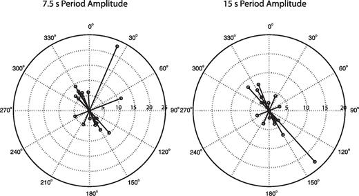
Maximum amplitude of Rayleigh wave signal in the NCF corrected for geometric spreading as a function of azimuth for 7.5 and 15 s period. Amplitude scale is arbitrary.
At the longer periods, >10 s, decreasing water depth causes the amplitude of Rayleigh waves to decrease as the phase velocity increases (Webb & Crawford 2010). The deep-water path (42–47) shows a broad-band signal from 6 to 25 s period relative to the spectrograms from shallower water paths such as 43–52, which has energy only to 13 s period. In addition, the two stations in water depths <1000 m, 40 and 48, show no coherent energy arriving at seismic velocities in any NCF as illustrated in Fig. 2(B, grey) for paths 40–45 and 48–52. Presumably at these shallow stations, non-seismic environmental sources dominate the pressure records. Although we prefer this explanation, we cannot rule out the possibility that above 10 s period the distribution of noise sources is heterogeneous, although the onshore and deep water station-to-station NCFs are fairly symmetric in this period range (amplitudes between positive and negative lags within a factor of 2, Fig. 5, 15 s period), with somewhat more energy propagating to the southwest.
The multiple arrivals visible in the spectrograms for the deep-water paths can be explained by coherent energy propagating across the array at super-Rayleigh wave and sub-Rayleigh wave velocities. The sub-Rayleigh wave group velocities are due to the DPG′s sensitivity to the propagation of ocean gravity waves (Webb 1998) and noise correlation in this case is capturing the ocean wave propagation. Increased noise from infragravity waves at the longer periods produces coherent arrivals in noise correlation if the infragravity wave field is coherent (Harmon et al. 2012). We note there are sub-seismic arrivals visible in the spectrograms at group arrivals <0.5 km s-’1. These signals may also interfere with the signals in the original time-series and degrade the coherence of the seismic signals. The super-Rayleigh wave group arrivals may be due to other phases, such as body waves propagating across the array or surface waves obliquely propagating to the interstation azimuth.
The DPG may not be ideally suited for ambient noise correlation studies in shallow water. The deep-water path, 42–47 produced a good dispersion curve similar to dispersion observed from noise correlation in the Pacific (Harmon et al. 2007). In shallower water (<1000 m), our study did not produce any usable signals (e.g. Fig. 1B, 40–45 and 48–52). However, noise correlation may work well on vertical components of broad-band OBS if the instrument has been corrected for ocean gravity wave contamination using the DPG (e.g. Crawford & Webb 2000).
4.2 Implications of across-arc shear velocity structure
In Fig. 4, the shear velocity structures we observe correspond with the expected geology of the trench-accretionary prism-arc system. We interpret our shear velocity models as representing three distinct types of crust, oceanic crust (cyan, 42–47) of the downgoing plate, crust of the accretionary prism (red, 42–52 and 43–47) and arc crustal material (black, BKNI–MNAI, BKNI–PSI and MNAI–PSI). Paths through similar crustal regions have similar velocity structure in the group dispersion (Fig. 4B) and in the shear velocity models (Fig. 4A) indicating that these results are robust and repeatable.
The accretionary prism appears to thicken rapidly as the water depth shallows between the stations by ∼2 km. In the accretionary prism shear velocity models (red and blue) we observe shear velocities in the upper 15 km that are consistent with consolidated sediments (2.36–2.80 km s-’1). In the path nearest the trench (42–47), we estimate the sediment package is ∼6 km thick, while in the 42–52 and 43–47 path velocity models, the sediments appear to be 14–16 km thick. These estimates are in good agreement with estimates of ∼5–12 km beneath the stations from active source experiments (Vermeesch et al. 2009; Henstock et al. 2010). At >15 km depth we believe the velocities in the models indicate the transition into the crystalline crust, and we note the velocities in this depth range are similar to those observed in our inferred arc crust (black Fig. 4) and path 42–47 and in the nearby local seismicity derived 1-D shear velocity models in Siberut/Mentawai Islands (green dashed line, Fig. 4) of Collings et al. (2012) and Sumatra (purple dashed line, Fig. 4) of Lange et al. (2010). In Sumatra, the arc crust in the Lange et al. (2010) model appears to be thicker.
The shear velocity structure presented for path 42–47 (cyan) provides a rare estimate of the shear velocity structure of the Indian Ocean crust and upper mantle. The path is averaging over a ridge segment and the edge of the subducted investigator fracture zone. The shear velocities in our preferred model are lower than expected from 10 to 25 km depth for oceanic crust and upper mantle (<4.0 km s-’1) even given the uncertainty from our Monte Carlo error estimation (<4.3 km s-’1). For similar aged lithosphere (47–50 Ma) in the Pacific, upper mantle shear velocities are ∼4.65 km s-’1 (Nishimura & Forsyth 1989) and recent global models at 70 km depth show the region to have velocities ∼4.3–4.5 km s-’1 (Kustowski et al. 2008). Low velocities are unlikely to be caused by heterogeneous source distributions, which tend to yield faster apparent group velocity. There are several possible explanations for the low shear velocities we observe: bias in the group velocity estimate due to multipathing and focusing effects caused by rapidly changing structure in the forearc, azimuthal anisotropy, thickened oceanic crust or serpentinization of the crust and upper mantle.
To evaluate the potential bias in our estimates due to the strong velocity gradients in the structure of the forearc, we compare the apparent group velocity of synthetic seismograms of waves propagating through a 2-D structure of a thickening accretionary wedge to the great circle path average velocity. We calculate the synthetic seismograms using the Gaussian beam method (Yomogida & Aki 1985), using one station as a source and the other as a receiver, to simulate the Green′s function between each station pair. In the model we assume a crustal thickness of 7 km, a sediment thickness that increases from 5 km at the trench to 15 km beneath the shelf, based estimates of depth to the plate boundary from active source experiments in the region (Vermeesch et al. 2009; Henstock et al. 2010). We find that deviations from the great circle path between the station pairs are small, with typical group velocity residuals of <0.03 km s-’1, with the largest errors of 0.05 km s-’1 occurring at periods where the group dispersion curves transition from sensitivity in the water/sediment layers to the crust/mantle layers in the 42–47 path (12–15 s depending on the model). These error estimates are within our dispersion error estimates and the error bars shown in Fig. 4 should accurately capture this variation.
Azimuthal anisotropy may explain some of the low velocities we observe, but it is unlikely that it can completely account for our observations. The oceanic lithosphere may have high azimuthal anisotropy with up to 3–5 per cent peak-to-peak anisotropy (Harmon et al. 2009) due to lattice-preferred orientation (LPO) of olivine with a fast direction in the fossil and/or present day plate motion vector. Alternately, serpentinization along normal faults may cause a azimuthal anisotropy of similar magnitude through shape preferred orientation of alternating layers of fast (unserpentinized) and slow (serpentinized crust) material and preferred orientation of antigorite, with a fast direction in the strike of the faults (Faccenda et al. 2008). SKS splitting results from station GSI on Nias, show trench perpendicular fast directions with a magnitude of 1.8 s delay (Hammond et al. 2010), suggesting our station-to-station paths are sampling the slow direction with 3–5 per cent anisotropy. The large error assigned to our measurements encompasses the variation potentially caused by anisotropy, so our upper limits may be closer to the isotropic average velocity. We cannot test hypothesis about the source of azimuthal anisotropy with the ambient noise dataset, but subsequent analyses of the teleseismic Rayleigh wave data may help determine the magnitude and direction of azimuthal anisotropy in the region.
We can effectively rule out the explanation of our observed low shear velocities as being due to a 15-km-thick crust. The crustal thickness is significantly greater than the global average of 6–7 km (Forsyth 1992) and we do not see any evidence for isostatic bathymetric anomalies associated with thickened crust.
The low shear velocities are likely due to serpentinization. The upper limit of our 95 per cent confidence region based on formal error analysis for our shear velocity inversion at ∼25 km is 4.07 km s-’1 and possibly up to 4.30 km s-’1 from the Monte Carlo estimates, which is consistent with 14–24 per cent serpentinization based on the empirical relationships of Christensen (Christensen 2004) for dunite to lizardite serpentinization at 1 GPa. While high, this estimate is in good agreement with the depth extent and degree of serpentinization estimated off the coast of Costa Rica and Nicaragua (Grevemeyer et al. 2007; Van Avendonk et al. 2011).
Serpentinization of the oceanic lithopshere near the Investigator fracture zone may help explain low seismic coupling, rupture segmentation and enhanced intermediate seismicity near the fracture zone. Faulting within the Investigator Fracture zone may have provided a local pathway for water, allowing for serpentinization of the crust and upper mantle (White et al. 1992). The serpentinized crust and mantle may be rheologically weaker, thus allowing the topography of the fracture zone to break aseismically, accommodating strain in the damage region and decoupling the region beneath the Batu Islands (Chlieh et al. 2008). The large damage zone may create a barrier to rupture by creating a weak zone unable to propagate rupture. In addition, the streaks of intermediate depth seismicity observed along the Investigator Fracture zone′s trace on the subducting plate may also be consistent with dewatering of the upper mantle of the downgoing plate as serpentinite becomes unstable (Fauzi et al. 1996; Lange et al. 2010).
In the upper 10–20 km, the offshore station-to-station paths are slower than the CRUST2.0 model (cyan dashed Fig. 4). The four models agree well below 20 km depth. Since a significant proportion of the crustal velocity structure is roughly 1 km s-’1 slower than the CRUST2.0 model, our models clearly provide an improvement over the global compilation.
The shear velocity structure determined for the onshore (black) station-to-station paths is generally consistent with the CRUST2.0 model (black dashed Fig. 4) with slight differences in velocity with depth. Given the large regions averaged in our model, these differences are probably not significant. Our results show a transition at 30 km depth that could be the Moho, but this may reflect the loss of resolution at depths >30 km in our models and a reversion to the starting model rather than real structure. The shear velocities observed on Sumatra are generally consistent with the geology of the island, that is, continental type arc crust, as discussed in previous studies (Sieh & Natawidjaja 2000).
5 Conclusions
Using Rayleigh wave group velocity dispersion from ambient noise cross correlation functions of onshore seismic data with an offshore ocean bottom DPG data, we estimated 1-D path averaged shear velocity models for the downgoing Indian oceanic crust, the upper crust of the accretionary prism and the crustal structure of Sumatra. We have shown the cross correlation of seismic noise is possible for onshore–offshore applications using a DPG, but we suggest that the effects measuring surface waves in a shallowing water layer may affect the ability of pressure records to resolve the full spectrum. We infer 14–24 per cent serpentinization of the upper mantle adjacent to the investigator fracture zone on the downgoing plate and a rapidly increasing sediment thickness in the accretionary wedge of 6–15 km. Our models for offshore shear velocity are substantially lower than CRUST2.0, so we suggest that in this region our models offer an improved estimate for the shear velocity.
Acknowledgements
This work was funded by the United Kingdom′s Natural Environment Research Council Grant NE/D004381/ and data provided by the Ocean Bottom Instrument Facility. We thank the PACIFIC 21 and GEOFON operators for making the data available. We thank the editor, Christine Thomas and Yingjie Yang and one anonymous reviewer for helpful and constructive comments.
References
