


Summary
Utilizing seismic refraction/wide-angle reflection data from 11 approximately in-line earthquakes, 2-D P- and S-velocity models and a Poisson′s ratio model of the crust and uppermost mantle beneath the southern Tien Shan and the Pamir have been derived along the 400-km long main profile of the TIPAGE (TIen shan-PAmir GEodynamic program) project. These models show that the crustal thickness varies from about 65.5 km close to the southern end of the profile beneath the South Pamir through about 73.6 km under Lake Karakul in the North Pamir, to about 57.7 km, 50 km south of the northern end of the profile in the southern Tien Shan. Average crustal P velocities are low with respect to the global average, varying from 6.26 to 6.30 km s-1. The average crustal S velocity varies from 3.54 to 3.70 km s-1 along the profile and thus average crustal Poisson′s ratio (σ) varies from 0.23 beneath the central Pamir in the south central part of the profile to 0.265 towards the northern end of the profile beneath the southern Tien Shan. The main layer of the upper crust extending from about 2 km below the Earth′s surface to 27 km depth below sea level (b.s.l.) has average P velocities of about 6.05-6.1 km s-1, except beneath the south central part of the profile where they decrease to around 5.95 km s-1. This is in contrast to the S velocities which range from 3.4 to 3.6 km s-1 and exhibit the highest values of 3.55-3.6 km s-1 where the P velocity is lowest. Thus, σ for the main layer of the upper crust is 0.26 beneath the profile except beneath the south central part of the profile where it decreases to 0.22. The low value of 0.22 for σ under the central Pamir, the along-strike equivalent of the Qiangtang terrane in Tibet, is similar to that within the corresponding layer beneath the northern Lhasa and southern Qiangtang terranes in central Tibet and is indicative of felsic rocks rich in quartz in the a state. The lower crust below 27 km b.s.l. has P velocities ranging from 6.1 km s-1 at the top to 7.1 km s-1 at the base. Further, σ for this layer is 0.27-0.28 towards the northern end of the profile but is low at about 0.24 beneath the central and southern parts of the profile, which is similar to the situation found in the northeast Tibetan plateau. The low values can be explained by felsic schists and gneisses in the upper part of the lower crust transitioning to granulite-facies and possibly also eclogite-facies metapelites in the lower part. Within the uppermost mantle, the average P velocity is about 8.10-8.15 km s-1 and σ is about 0.26. Assuming an isotropic situation, then a relatively cool (700-800°C) uppermost mantle beneath the profile is indicated. This would in turn indicate an intact mantle lid beneath the profile. An upper mantle reflector dipping from 104 km b.s.l., 120 km from the southern end of the profile to 86 km b.s.l., 155 km from the northern end of the profile has also been identified. The preferred model presented here for the crustal and lithospheric mantle structure beneath the Pamir calls for nearly horizontal underthrusting of relatively cool Indian mantle lithosphere, the leading edge of which is outlined by the Pamir seismic zone. This cool Indian mantle lithosphere is overlain by significantly shortening, warm Asian crust. The Moho trough that is a feature seen beneath some other orogenic belts, for example the Alps and the Urals, beneath the northern Pamir may mark the southern tip of the actively underthrusting Tien Shan crust along the Main Pamir thrust.
Introduction
The Pamir and Tien Shan comprise Earth′s largest and most active intra-continental orogen and form part of the India-Asia collision zone. The Pamir is situated in the western part of the Pamir-Tibet-Himalaya orogenic system at the tip of the western Indian promontory (Fig. 1). The southern Tien Shan are separated from the northern Pamir by the intra-montaine Alai valley, which connects the Tarim basin in the east with the Tajik basin, thrust-fold belt in the west. With respect to Tibet, the Pamir has accommodated Cenozoic shortening between India and Asia in about 50 per cent of the orogenic width. As a result a thick crust and high plateau, similar to Tibet, have formed. Presently, the Pamir and Tien Shan are shortening at up to 20 mm a-1, with 10-15 mm a-1 of this shortening being accommodated across the boundary between the northern Pamir and the Alai valley (Reigber et al. 2001; Mohadjer et al. 2010; Zubovich et al. 2010).
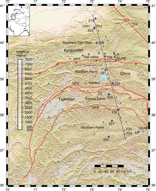
Location map of the seismological stations (blue, black and green crosses) and 11 earthquakes (blue circles) used in this study, with topography from the Shuttle Radar Topography Mission (SRTM). TIPAGE stations are marked as blue crosses, German Task Force stations are marked as black crosses and station OHH of the digital network of the Kyrgyz Republic is marked as a green cross. The red lines mark major tectonic boundaries. In the inset the outline of Tibet, the Pamir and the Tien Shan, as defined by the 3000 m contour, is shown. Key: MPF, Main Pamir Fault; NPS, Northern Pamir Suture; TS, Tanymas Suture; RPS, Rushan Psart Suture; TFF, Talas Fergana Fault.
In the summer of 2008, an array of 40 seismological stations was installed in the Pamir and southern Tien Shan as part of the TIPAGE (TIen shan-PAmir GEodynamic program) project (Fig. 1). The array remained in this configuration which included a main profile of 24 stations, until the summer of 2009. Between the summers of 2009 and 2010 the array was re-configured such that fewer stations were deployed along the main profile. One of the major aims of the main profile of 24 stations was to obtain a receiver function section of the crust and upper mantle down to about 700 km depth (Sippl et al. 2010; Schneider et al. 2011). One of the main aims of the array between the summers of 2009 and 2010 and the 16 stations deployed off the main profile between the summers of 2008 and 2009 was to get a more accurate picture of the distribution of regional seismicity than previous studies (Sippl et al. 2010, 2011; Schurr et al. 2011). A further aim of the array is to derive 3-D models of the various physical parameters, for example compressional (P) and shear (S) velocities and Poisson′s ratios beneath the region based on local and teleseismic earthquake tomography. Work is still in progress on all of these aims and should provide material for forthcoming publications. One of the subsidiary goals of having the array configured as it was between the summers of 2008 and 2009 was the hope to record some crustal earthquakes along the main profile and to re-locate these earthquakes using the whole array. It was then hoped to use these re-located earthquakes for an analysis of the wide-angle seismic phases recorded along the main profile, in order to have a method in addition to the receiver functions and the tomography for obtaining P- and S-wave velocities of the crust and uppermost mantle. Such a strategy has already been used to derive a S-wave velocity model for central Tibet (Mechie et al. 2004). Blümling & Prodehl (1983) also used a similar strategy to determine the P-wave velocity model for a seismic profile in central California. The TIPAGE array configuration between the summers of 2008 and 2009 consisted of a NNW-SSE trending main profile along which 24 stations at a nominal spacing of 15 km were deployed and 16 off-line stations, of which 13 were deployed to the west of the main line and three to the east (blue crosses, Fig. 1). This array was augmented by the deployment of seven additional stations (black crosses, Fig. 1) in the Alai valley following the destructive Mw= 6.6 Nura earthquake of 2008 October 5. Additionally, the data from the station OHH (green cross, Fig. 1) from the digital network of the Kyrgyz Republic were utilized for one event.
Previous deep seismic work in the region, summarized by Burtman & Molnar (1993), includes a controlled-source wide-angle seismic profile completed in 1977 (Beloussov et al. 1980). Along that part of the earlier profile which coincides with the TIPAGE main profile, six shot-points were completed and the station spacing was about 10 km. Beloussov et al. (1980) did not show any seismograms, but only traveltime picks. The model of Beloussov et al. (1980) showed crustal thickness varying from 51 km below sea level (b.s.l.) at the northern end of the TIPAGE main profile to 66 km b.s.l. at the southern end of the TIPAGE main profile with a local deepening to about 76 km b.s.l. beneath Lake Karakul. Beloussov et al. (1980) also reported uppermost mantle P velocities of 8.1 km s-1 at the northern end of the TIPAGE main profile and 8.05 km s-1 at the southern end of the profile. No estimates were given for the region in between. The new seismic refraction / wide-angle reflection data presented in this study allow the derivation of P and S velocity and Poisson′s ratio models for the crust and uppermost mantle and their first-order N-S variations beneath the southern Tien Shan and the Pamir. This leads to the conclusion about a model in which the warm Asian crust of the Pamir is underlain by relatively cool Indian mantle lithosphere.
Geological setting
Although the Pamir-Tien Shan share many geodynamic aspects with the Tibet-Himalaya orogenic system, several features of the Pamir and southern Tien Shan are unique (Figs 1-2). The Pamir has been displaced northward by about 600 km with respect to Tarim (Burtman & Molnar 1993), thrusting over virtually all the Tarim basin that is up to 1000 km wide and mostly undeformed north of Tibet. The Pamir forms one of Earth′s most spectacular oroclines with the active frontal ranges bending nearly 180° from northern Afghanistan to the western Kunlun of China; deformation is truly 3-D plus time. The Hindu Kush and the Pamir were interpreted to include two continental subduction zones, the Hindu Kush and Pamir seismic zones, resolvable by seismicity and tomography (Burtman & Molnar 1993; Pegler & Das 1998; Koulakov & Sobolev 2006; Negredo et al. 2007). The southern Tien Shan and the Pamir embrace a huge depositional system and foreland fold-thrust belt, the Tajik basin. To the east, the western end of the Alai valley has been more or less completely overthrust by 300-400 km of convergence between the Pamir and the Tien Shan (Burtman 2000). About 200 km further east, however, Coutand et al. (2002) found displacement rates over the past 25 Ma to be about one order of magnitude smaller than those implied by Burtman & Molnar (1993) and Burtman (2000). Both the Tajik-basin deposits and the widespread outcrop of intermediate temperature/intermediate pressure rocks, the Pamir crystalline basement domes, within the Pamir testify to substantial erosion of the orogen (Schwab et al. 1980, Hubbard et al. 1999). The N-S extent of the Pamir is about 500 km, compared with up to 1300 km for Tibet, yet both have absorbed around 1800-2100 km of Cenozoic N-S shortening (Le Pichon et al. 1992; Johnson 2002). Tibet and the Pamir both stand 4-5 km high (Fielding 1996), which in Tibet is supported by a 70-80 km thick crust (Kind et al. 2002; Mechie et al. 2011). Consequently, compared to Tibet, the Pamir has either undergone more lateral extrusion of crust, more erosional unroofing or greater loss of continental crust into the mantle.
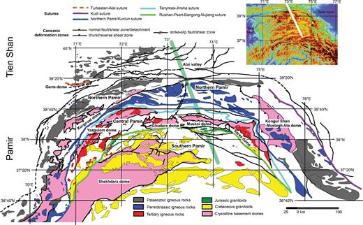
Simplified geological map of the southern Tien Shan and the Pamir, including crystalline basement domes, Palaeozoic-Tertiary magmatic rocks, Palaeozoic-Mesozoic sutures and major Cenozoic deformation zones. The thick line marks the TIPAGE profile. Map strongly modified from Vlasov et al. (1991), Schwab et al. (2004) and our own observations.
As in Tibet, the Pamir is composed of broadly E-W trending belts formed by successive collisions during the Late Palaeozoic-Mesozoic (Schwab et al. 2004). The northern Pamir is a Palaeozoic arc and subduction-accretion complex like the Kunlun arc and Hoh Xil-Songpan-Ganze terrane of northern Tibet, the central Pamir comprises Palaeozoic-Jurassic platform rocks correlative with the Qiangtang terrane, and the southern Pamir consists of Palaeozoic-Mesozoic meta-sedimentary rocks, rare Proterozoic gneisses, and voluminous Cretaceous-Palaeogene granitoids, equivalent to the Lhasa terrane in Tibet. Unlike Tibet, these belts have been bent into an orocline (Burtman & Molnar 1993). The Pamir seismic zone is understood to mark about 300 km southward subduction of Asian lithosphere (Hamburger et al. 1992; Burtman & Molnar 1993), although some workers (Pegler & Das 1998; Pavlis & Das 2000) have claimed that it represents overturned northward subducting Indian lithosphere. In contrast, the Hindu Kush intermediate-depth seismicity is interpreted to mark around 700 km of subducted Indian lithosphere dipping at about 80° to the north (Negredo et al. 2007). However, east of the Pamir, Indian lithosphere is ‘subducting’ beneath Tibet almost horizontally (Kumar et al. 2006; Jiménez-Munt et al. 2008) and may underlie most of western Tibet (Li et al. 2008; Zhao et al. 2010).
Earthquake selection & re-location
As a result of the examination of the U.S. Geological Survey earthquake catalogue and running an event detection algorithm on the continuous data collected between the summers of 2008 and 2009, 10 crustal events and one event in the top 10-15 km of the mantle were selected for re-location and further analysis of the wide-angle phases. The southernmost event (no. 3) was the only event in the catalogue near the southern end of the profile and, in fact, the catalogue location placed the event about 40 km south of the south edge of the array (Fig. 1). Visual inspection of the first P arrival data showed that the waves from this event arrived at station SHA8 first followed by stations P23 and P24. The other two events (nos. 225 and 227) in the southern part of the profile (Fig. 1) were not in the catalogue but were found by the event detection algorithm. One event (no. 225) was suspected to originate in the mantle from visual inspection of the S-P arrival times and the other (no. 227) showed the strongest signal to noise ratios of the remaining few events along this part of the profile. The five small events (nos. 229, 230, 232, 236 and 281) with magnitudes less than 3, were all found by the event detection algorithm. The event (no. 166) in the Alai valley (Fig. 1) is one of many earthquakes that occurred in this region between the summers of 2008 and 2009, especially following the Mw= 6.6 Nura earthquake of 2008 October 5. This event was chosen as it was one of the larger events which occurred closer to the profile in this region rather than being closer to the station NUR8 at Nura. The northernmost two events (nos. 219 and 220) were two of three events in the catalogue near the northern end of the profile (Fig. 1). Together with the crustal events at the southern end of the profile described above, they are the only events near the profile which are large enough to show clear signals at far enough offsets and thus to provide reliable information on the whole crustal thickness and velocity structure. Event 220 was chosen for re-location and further analysis as it was found to lie within the array when it was re-located. Event 219 was chosen for re-location and further analysis as it had the best signal to noise ratios especially at the furthest away stations of the array and as it showed good secondary P and S phases. For this event, the data from station OHH at Osh were also utilized. These 11 events result in a fairly even source spacing of approximately 40 km in the crust along the profile. A significantly smaller source spacing with such an even distribution of sources in the crust is not possible due to the scarcity of crustal earthquakes in the south central part of the profile between event 227 and event 230 (Fig. 1).
For the 11 selected events the onset times of the first P- and S-wave arrivals were picked and a pick quality was assigned. Additionally the polarity of the first P-wave arrivals was noted. The P-wave arrivals were picked on the vertical component while the S-wave arrivals were picked on the horizontal components of ground motion. In most cases the arrivals were picked on unfiltered traces. For the location procedure, the HYPO71PC computer program (Lee & Valdés 1985) was used. This program requires a 1-D P-velocity model and a Vp/Vs (P velocity/S velocity) ratio. Two 1-D P-velocity models were tried (Table 1). One was based on a model for northern Tibet about 2000 km to the east, but with a 5 km shallower crust-mantle boundary (Moho). The other was that for the 2 × 2 degree region centred at 73°E, 39°N taken from the CRUST2.0 global model (Bassin et al. 2000). In order to determine a Vp/Vs ratio, and also to aid in checking the trade-off between the origin time and the depth, Wadati diagrams were made for each of the events. For the five northern events, Vp/Vs ratios of 1.72-1.75 were obtained (Table 2). For the six southern events, the five in the crust provided Vp/Vs ratios of 1.68-1.72 and that (no. 225) in the mantle provided a Vp/Vs ratio of 1.78, reflecting mainly the Vp/Vs ratio in the uppermost mantle. The Vp/Vs ratio for a Poisson solid of 1.73 was utilized in the location procedure, which ratio is close to the average Vp/Vs ratio for the 11 events of 1.72. For six of the 11 events, including all five events for which the location procedure utilized phases penetrating into the lower crust and uppermost mantle, the location from the 1-D model based on that for northern Tibet gave a root mean square (rms) traveltime residual which was up to 0.17 σ smaller than that for the 1-D model taken from the CRUST2.0 global model. This was due to the fact that the lower crust in the 1-D model based on that for northern Tibet has a lower P velocity than the lower crust in the 1-D model taken from the CRUST2.0 global model. Further, for the other five events the difference in the rms traveltime residual between the locations from the CRUST2.0 global model and the northern Tibet model was not greater than 0.05 s. The locations derived using the 1-D model based on that for northern Tibet were used in the further analysis. Ten of the 11 events were located within the network of stations. Only event 219 was located outside the network, about 32 km north of station P01 and 26 km NE of station OHH. However, due to the fact that the polarities of the 1st arrival P waves on all three components at the northernmost six stations are in agreement with the location and the standard errors for the epicentre and the focal depth are less than 1.5 km, it is thought that this event can be used in the further analysis. The standard error of the epicentre for all events is less than 1.5 km. The standard error of the focal depth is less than 2.0 km for all events except 227. However, these values are somewhat optimistic as, for example, errors in the 1-D P velocity model and Vp/Vs ratio are not taken into account. Tests using the two velocity models described above (Table 1), different Vp/Vs ratios (Table 2) and different subsets of the data suggest that the standard errors for the epicentre and the focal depth are about 3-4 and 5-6 km, respectively. Ten of the 11 events are located in the upper 20 km of the crust. No lower crustal events within the vicinity of the profile were found.
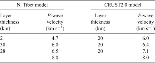
One-dimensional velocity-depth models for Pamir region.

Data and phase correlations
Following the location procedure, new record sections were constructed for the vertical and horizontal components of ground motion for each of the 11 events (Figs 3-8). Due to the better alignment of phases, this allowed additional traveltime picks to be made at larger distances where the signal to noise ratio is somewhat poorer and also for secondary reflected phases to be picked in the P and/or S wavefields for event nos. 219, 220, 225, 227 and 236.
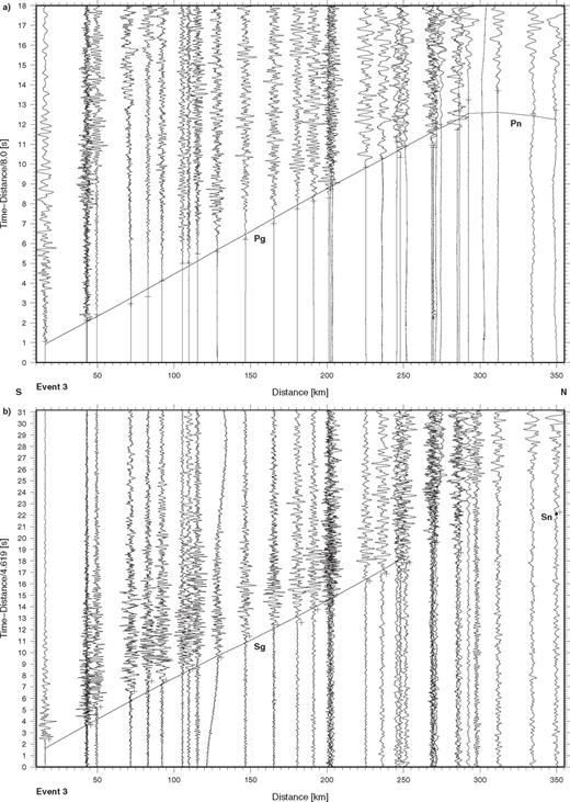
Seismic data from event no. 3 recorded along the TIPAGE main profile. The record sections show (a) the vertical component of P-wave motion reduced with a velocity of 8 km s-1 and (b) the N-S horizontal (approximately radial) component of S-wave motion reduced with a velocity of 4.62 km s-1. Each trace is normalized individually and some traces, especially at larger distances, are low pass filtered at 5 Hz. Lines (dots) represent phases calculated from the models in Figs 10a-b, while crosses (slightly offset in b) represent observed traveltimes. Key: Pg, first arrival refraction through the upper crust; Pn, first arrival refraction through the uppermost mantle; Sg, S-wave refraction through the upper crust; Sn, S-wave refraction through the uppermost mantle.
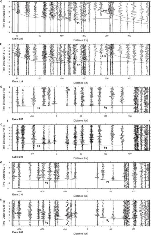
Seismic data from event nos. 225, 232 and 230 recorded along the TIPAGE main profile. The record sections show (a) the vertical component of P-wave motion for event no. 225 reduced with a velocity of 8 km s-1, (b) the E-W horizontal (approximately tangential) component of S-wave motion for event no. 225 reduced with a velocity of 4.62 km s-1, (c) the vertical component of P-wave motion for event no. 232 reduced with a velocity of 6 km s-1, (d) the N-S horizontal (approximately radial) component of S-wave motion for event no. 232 reduced with a velocity of 3.46 km s-1, (e) the vertical component of P-wave motion for event no. 230 reduced with a velocity of 6 km s-1 and (f) the N-S horizontal (approximately radial) component of S-wave motion for event no. 230 reduced with a velocity of 3.46 km s-1. The data are processed and presented as in Fig. 3, except that the data for event nos. 230 and 232 have been bandpass filtered from 1 to 20 Hz. Key: see Fig. 3 and P1P- uppermost mantle P-wave reflection, S1S- uppermost mantle S-wave reflection.
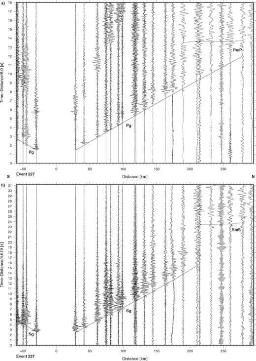
Seismic data from event no. 227 recorded along the TIPAGE main profile. The record sections show (a) the vertical component of P-wave motion reduced with a velocity of 8 km s-1 and (b) the E-W horizontal (approximately tangential) component of S-wave motion reduced with a velocity of 4.62 km s-1. The data are processed and presented as in Fig. 3, except that in this case some of the traces, especially at larger distances, are bandpass filtered from 0.35 to 5 Hz. Key: see Fig. 3 and PmP-P-wave reflection from Moho, SmS-S-wave reflection from Moho.
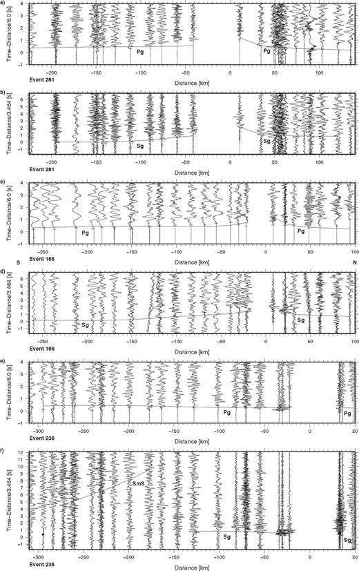
Seismic data from event nos. 281, 166 and 236 recorded along the TIPAGE main profile. The record sections show a) the vertical component of P-wave motion for event no. 281 reduced with a velocity of 6 km s-1, (b) the E-W horizontal (approximately tangential) component of S-wave motion for event no. 281 reduced with a velocity of 3.46 km s-1, (c) the vertical component of P-wave motion for event no. 166 reduced with a velocity of 6 km s-1, (d) the N-S horizontal (approximately radial) component of S-wave motion for event no. 166 reduced with a velocity of 3.46 km s-1, (e) the vertical component of P-wave motion for event no. 236 reduced with a velocity of 6 km s-1 and (f) the E-W horizontal (approximately tangential) component of S-wave motion for event no. 236 reduced with a velocity of 3.46 km s-1. The data are processed and presented as in Fig. 3, except that the data for event nos. 236 and 281 have been bandpass filtered from 1 to 10 Hz and 1 to 20 Hz, respectively. Key: see Figs 3 and 5.
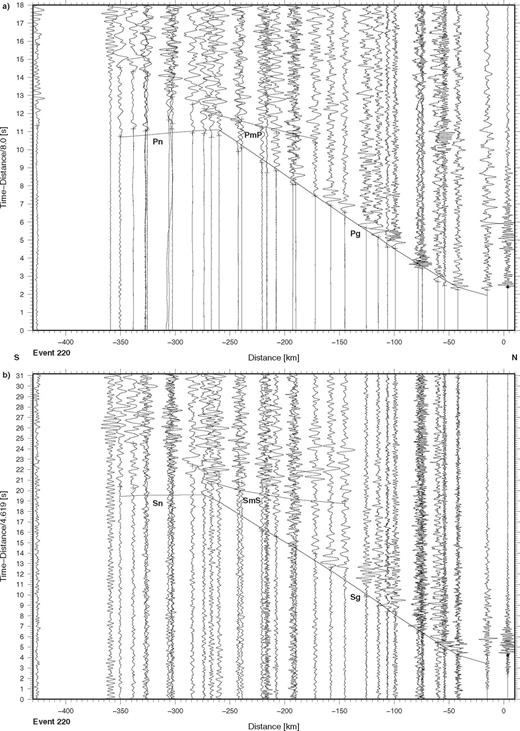
Seismic data from event no. 220 recorded along the TIPAGE main profile. The record sections show (a) the vertical component of P-wave motion reduced with a velocity of 8 km s-1 and (b) the E-W horizontal (approximately tangential) component of S-wave motion reduced with a velocity of 4.62 km s-1. The data are processed and presented as in Fig. 3. Key: see Figs 3 and 5.
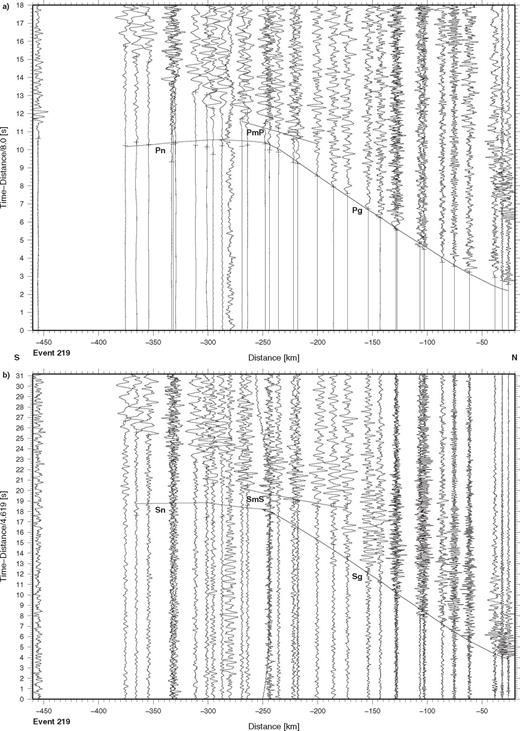
Seismic data from event no. 219 recorded along the TIPAGE main profile. The record sections show (a) the vertical component of P-wave motion reduced with a velocity of 8 km s-1 and (b) the N-S horizontal (approximately radial) component of S-wave motion reduced with a velocity of 4.62 km s-1. The data are processed and presented as in Fig. 3. Key: see Figs 3 and 5.
On the vertical component of ground motion for event 3 (Fig. 3a), in which the P wavefield can mainly be seen, the direct/refracted phase, Pg, through the upper crust forms the first arrivals out to about 300 km distance with an average apparent velocity close to 6 km s-1. Beyond 300 km distance some arrivals belonging to the refracted phase, Pn, through the uppermost mantle may be correlated. No reflections can be observed in this record section. On the horizontal components of ground motion, in which the S wavefield can mainly be seen, the direct/refracted phase, Sg, through the upper crust can be correlated out to about 250 km distance with an average apparent velocity close to 3.5 km s-1. Additionally, there is one arrival at 350 km distance on the N-S (almost radial) component (Fig. 3b) which may correspond to the refracted phase, Sn, through the uppermost mantle. As with the P wavefield, no reflections can be correlated in the S wavefield.
As event 225 is located in the uppermost mantle only phases which travel at least partly through the mantle can be recognized on the record sections (Figs 4a-b). On the vertical component of ground motion (Fig. 4a) only Pn appears as the first arrival with an average apparent velocity of about 8.1 km s-1 beyond distances of about 170 km. At distances smaller than about 170 km the effect of the depth of the event influences the apparent velocity of Pn. At distances greater than 220 km a strong secondary phase which is here interpreted as a reflection, P1P, from within the uppermost mantle, can be correlated. On the horizontal components of ground motion Sn can be correlated (Fig. 4b) with an average apparent velocity of about 4.6 km s-1 beyond distances of about 170 km. Further, the S-wave equivalent, S1S, of the P reflection from within the uppermost mantle can also be easily recognized in the horizontal components of ground motion.
In the P wavefield for event 227 (Fig. 5a), only Pg appears as the first arrival, out to about 280 km distance. Some secondary arrivals which have been correlated as the reflected phase, PmP, from the Moho can be recognized, beyond about 180 km distance. In the S wavefield (Fig. 5b), Sg can be correlated out to about 200 km distance. As in the case of the P wavefield, some later arrivals which have been correlated as the reflected phase, SmS, from the Moho can be seen beyond about 200 km distance.
For events 232, 229, 230, 281, 166 and 236 only Pg appears as the first arrival out to a maximum distance of about 260 km (Figs 4c and e and 6a, c and e). No reflections have been correlated in the P wavefields for these events. In the S wavefields (Figs 4d and f and 6b, d and f), Sg can also be correlated out to a maximum distance of about 260 km. In contrast to the P wavefields, it has been possible to correlate some secondary arrivals beyond about 175 km distance, in the S wavefield of event 236, as the reflected phase, SmS, from the Moho (Fig. 6f).
The record sections for events 220 (Fig. 7) and 219 (Fig. 8) look very similar. In the P wavefields for both events Pg can be recognized as the first arrival out to 250-260 km distance with an average apparent velocity close to 6 km s-1, beyond 60 km distance. At distances smaller than 60 km, the effect of the depths of the events influence the apparent velocity of Pg. Beyond 250-260 km distance Pn can be correlated as the first arrival with an average apparent velocity of about 8 km s-1. In the S wavefields for both events Sg can be correlated out to 220-250 km distance with an average apparent velocity close to 3.5 km s-1 beyond 60 km distance. Beyond about 250 km distance some arrivals which have been recognized as Sn on the horizontal components have been recognized. On the P- and S-wave record sections for both events, secondary arrivals can be recognized. Out to about 280 km distance these have been correlated as the reflected phases, PmP and SmS, from the Moho.
1 1-D modelling
One of the problems with the 1-D model used to locate the earthquakes is that it produces theoretical phases which are not observed in the data (Fig. 9a). For example, it produces a prominent PiP phase between the Pg and PmP phases beyond distances of about 120 km. Such a phase is not recognized in the observed data. Thus, some 1-D traveltime and amplitude calculations were made in order to search for a simple model which only produced the phases observed in the data. In doing so it was not the purpose to do a full waveform inversion as the data are not closely enough sampled to warrant such an approach. Rather, the purpose was only to make sure that the model did not produce strong phases which one might have expected to recognize in the observed data. In calculating the theoretical seismograms for 1-D models, the reflectivity method (Fuchs & Müller 1971) with a uniform point source was used. Further, S velocities were set to be equal to the P velocities divided by 1.732 and densities were calculated using the relationship of Birch (1961). One possibility to avoid the problem of too many phases is to omit an intra-crustal boundary. However, this produces an energy distribution for the PmP phase which is significantly later than the main energy in the observed data (Fig. 9b). Another possibility to avoid this problem is to include a significant velocity gradient in the lower crust. This produces much energy in the triplications at around 250 km distance and also a distribution of traveltimes and energy for the PmP phase which agrees with those in the observed data (Fig. 9c). Thus, for the 2-D modelling, a lower crust with a gradient from 6.1 km s-1 at the top to 7.1 km s-1 at the base was utilized. Unfortunately, the observed data are too coarsely sampled, to recognize with confidence the triplications which are produced in the theoretical seismograms for this model. In addition, in creating the 1-D model to be used as a basis for the 2-D modelling (Fig. 9c), a very small velocity gradient (0.0036 s-1) in the upper crust and a modest velocity gradient (0.0062 s-1) in the upper mantle were introduced. Introducing these gradients provides better qualitative agreement between the observed and theoretical amplitude ratios for Pg/PmP and Pn/Pg or PiP. In particular, it results in small but visible amplitudes for the Pn phase compared to the later phases (Fig. 9c). This is in better agreement with the observed data (e.g. Fig. 8a), than amplitudes for the Pn phase which are too small to be recognizable when compared to the later phases (Fig. 9a-b).
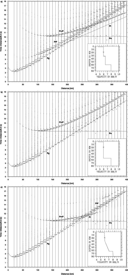
(a) Synthetic seismograms and one-dimensional P-velocity model (N. Tibet model, see Table 1) used for the 1-D re-location of the earthquakes. (b) Synthetic seismograms and 1-D P-velocity model with essentially no lower crust. (c) Synthetic seismograms and 1-D P-velocity model used as the basis for the 2-D models in this study. See text for further discussion. The synthetic seismogram sections, calculated with the reflectivity method, show the vertical component of P-wave motion and are reduced with a velocity of 8 km s-1 and each trace is normalized individually. Continuous lines represent phases calculated from the 1-D models in the insets. Crosses represent observed traveltimes for event no. 219. Key: see Figs 3 and 5 and PiP-P-wave reflection from the boundary between the upper and lower crust, Pi-P-wave refraction through the lower crust.
2 2-D modelling
2-D modelling was carried out by inversion of the P and S traveltimes supplemented by forward modelling of the amplitudes of the P phases. For the modelling of the traveltimes, the forward problem was solved by finite-differences ray-tracing based on the eikonal equation (Vidale 1988; Podvin & Lecomte 1991; Schneider et al. 1992) for the first arrival refracted phases and by classical ray-tracing techniques (Cervený 1977) for the reflected phases. A grid size of 50 × 50 m was used for the finite-differences ray-tracing. Partial derivatives of the calculated traveltimes with respect to the velocity and/or interface nodes were then derived using the techniques described by Lutter & Nowack (1990), Lutter et al. (1990) and Zelt & Smith (1992). Subsequently, a damped least-squares inversion (see, e.g. Zelt & Smith 1992) was carried out to obtain updates for the velocity and/or interface nodes, and the forward and inverse problems were repeated until an acceptable convergence between the observed and calculated traveltimes was obtained. Then, the amplitudes were calculated using an explicit finite-differences approximation of the wave equation for 2-D heterogeneous media (Kelly et al. 1976) with transparent boundary conditions (Reynolds 1978) and implemented by Sandmeier (1990). Again a grid size of 50 × 50 m was utilized in calculating the amplitudes, which allowed for frequencies of up to about 4 Hz to be calculated. The vertical velocity gradients were then adjusted, if necessary, and the traveltime inversion repeated.
For the 2-D modelling, the epicentres derived above for the 11 events (Table 2) were projected at right angles onto the line of the profile which is N14°W (Fig. 1). The origin times and depths derived above for the 11 events (Table 2) were also utilized, except for event 3 for which the depth was moved upwards by 6 km. This was done due to the following reasons. Following the location of this event and the construction of a new record section, it was possible to pick the first P arrival at the two most distant receivers (Fig. 3a). First attempts to carry out the 2-D modelling using the depth derived above for event 3 always produced very early synthetic traveltimes for the Pn phase. It was then noticed that by decreasing the depth for event 3, one could significantly delay the Pn phase without advancing the Pg phase too significantly. For example, by decreasing the depth by 5 km, the Pn phase is delayed by 0.55 σ and the Pg phase is advanced by less than 0.10 σ for distances greater than 40 km. Finally, a depth decrease of 6 km was chosen which brings the depth for event 3 to within 0.5 km of the depth for event 227, which is the other crustal event along the southern part of the profile used in this study.
The traveltime modelling was done using a top-to-bottom approach in three steps for the P traveltimes and two steps for the S traveltimes. In total, 261 P and 205 S traveltimes were used in the inversion (Table 3). The P-velocity model contains 11 independent velocity and interface depth parameters while the S-velocity model contains seven independent velocity parameters (Tables 4 and 5). In the first step to derive the P-velocity model (Fig. 10a), 187 Pg phase traveltimes were utilized to determine the velocity structure in the main upper crustal layer between 2 km below the Earth′s surface and 27 km depth b.s.l. In the second step, 22 PmP phase and 46 Pn phase traveltimes were used to derive the average P velocity of the lower crust, the Moho structure and an average Pn velocity. In the third step, 6 P1P phase traveltimes were utilized to derive the depths of the mantle reflector. A laterally homogeneous initial Pg velocity of 5.95 km s-1 at -2 km depth and a vertical velocity gradient of 0.0036 s-1 in the upper crust was employed in the first step and the velocities at the top and bottom of the main upper crustal layer were constrained to be updated by the same amount in each iteration of the inversion. Four independent velocity nodes were utilized in this inversion step (Table 4) as the outer two nodes at both ends of the profile were constrained to be updated by the same amount. The 2-km-thick top layer with a P velocity of 4.7 km s-1 was held fixed in the 2-D modelling. In the second step, the initial P velocity of the lower crust was set to be 6.1 km s-1 at the top of the lower crust at 27 km b.s.l. and 7.1 km s-1 at the base of the lower crust. The Moho was set initially to be at 63 km depth b.s.l., and an initial Pn velocity of 8.0 km s-1 at the Moho and a vertical velocity gradient of 0.0062 s-1 in the uppermost mantle was employed. The velocities at the top and base of the lower crust were constrained to be updated by the same amount while the velocities in the uppermost mantle were constrained to be updated such that the vertical velocity gradient was maintained. Thus, in this inversion step, one velocity node in the lower crust and one velocity node in the uppermost mantle were employed, in addition to three Moho depth nodes (Table 4). The top of the lower crust was held fixed at 27 km depth b.s.l. throughout the 2-D modelling. In the third step the upper mantle reflector was initially at 101.5 km depth b.s.l. In this step, two interface depth nodes at 120 and 245 km along the profile were used in the inversion (Table 4).
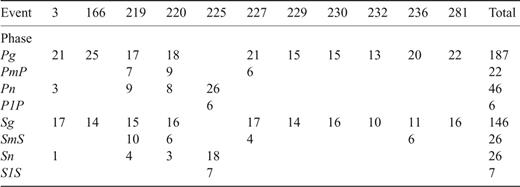
Number of traveltimes picked for each phase from each event.


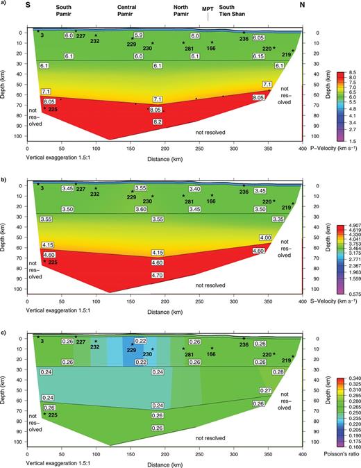
Two-dimensional (a) P-wave velocity, (b) S-wave velocity and (c) Poisson′s ratio models along the TIPAGE main profile. Velocities are accurate to the nearest 0.05 km s-1. The positions of the 11 events used in the modelling are marked by black stars. Positions of the Moho from Beloussov et al. (1980) are marked by small black circles. Key: MPT, Main Pamir Fault.
The S velocity model (Fig. 10b) was derived in two steps. In the first step, 146 Sg phase traveltimes were utilized to determine the velocity structure in the main upper crustal layer between 2 km below the Earth′s surface and 27 km depth b.s.l. As in the case of the inversion for P velocities, four independent velocity nodes were utilized (Table 4). Again the 2-km-thick top layer was held fixed in the inversion with a S velocity of 2.71 km s-1. In the second step, 26 SmS phase, 26 Sn phase and 7 S1S phase traveltimes were used to derive the velocity structure in the lower crustal layer between 27 km depth b.s.l. and the Moho and an average Sn velocity. Two velocity nodes in the lower crust and one velocity node in the uppermost mantle were employed in this inversion step (Table 4). In both inversion steps, the boundary depths were adopted from the final P-velocity model and initial S velocities were set to be equal to the final P velocities divided by 1.732.
Up to six iterations were required in each step of the inversion in order to reduce the average absolute traveltime residuals to the point where no further improvement occurred (Table 5). The χ2 values (Table 5) are always greater than 1, except in the case of the inversion of the P1P phase data, indicating that the data are certainly not over fitted. It is also possible that, in some cases, the error estimates for the picked traveltime data are too optimistic. Inspection of the resolution matrices shows that all the parameters have a resolution greater than 0.5 and all off-diagonal elements of the resolution matrices are at least a factor of six smaller than the diagonal elements. The ray diagrams (Fig. 11) show which regions of the model are better covered.

Ray diagrams from the final models shown in Figs 10(a-b) for the (a) Pg phase, (b) PmP, Pn and P1P phases, (c) Sg phase and (d) SmS , Sn and S1S phases.
For the main upper crustal layer, P velocities are relatively constant at 6.0-6.05 km s-1 at the top of the layer, 2 km below the surface, except beneath the south central part of the profile where they decrease to 5.9 km s-1. Corresponding S velocities range from 3.4 to 3.55 km s-1 with the highest values of 3.55 km s-1 being obtained where the Pg velocity is lowest. This then results in a P-velocity/S-velocity (Vp/Vs) ratio and Poisson′s ratio (σ) in the upper crust of 1.747-1.763 (σ= 0.26) except beneath the central Pamir where values of 1.664-1.665 (σ= 0.22) are encountered (Fig. 10c). An inversion was carried out in which an extra node was introduced in the upper crust for the inversion of the P velocities. However, this inversion resulted in a P-velocity distribution that showed a tendency to oscillate and the rms traveltime residual showed no improvement with respect to the final model (Fig. 10a). The inversion for the average P velocity in the lower crust resulted in essentially no change with respect to the initial values. This was most fortunate as if there had been a tendency for the average P velocity in the lower crust to have increased during the inversion, then a strong intracrustal reflection, PiP, would have been generated which is not observed in the data (cf.Fig. 9a). The inversion for the S velocity in the lower crust resulted in Vp/Vs for this layer of 1.709-1.712 (σ= 0.24) in the southern and central parts of the profile, increasing to 1.794-1.818 (σ= 0.27-0.28) near the northern end of the profile.
One of the first tasks during the second step of the inversion for the P-velocity model was to determine the best horizontal coordinate of the third Moho depth node, approximately in the middle of the profile. This was accomplished by inverting the 68 PmP and Pn traveltimes for the P velocity of the lower crust, the Moho depths and the average Pn velocity, but with several different values of the horizontal coordinate of the third Moho depth node and then choosing the solution for which the rms traveltime residual was smallest. It turned out that to within the nearest 10 km, 190 km from the southern end of the profile gave the best result. The Moho dips from 55.7 km depth b.s.l., 50 km south of the northern end of the profile to 69.6 km depth b.s.l., 10 km south of the middle of the profile beneath Lake Karakul in the northern Pamir. It then shallows to 61.1 km depth b.s.l. close to the southern end of the profile. Taking the topography into account, this results in total crustal thicknesses of about 57.7 km, 50 km south of the northern end of the profile, about 73.6 km under Lake Karakul in the northern Pamir and about 65.5 km close to the southern end of the profile. It turned out that the Moho trough almost below the middle of the profile has an effect on the amplitudes of the Pn phase and for this reason the vertical P velocity gradient in the uppermost mantle was increased to 0.01 s-1 following an initial set of traveltime inversions utilizing the gradient of 0.0062 s-1 derived from the 1-D modelling. Additionally, an inversion was attempted in which the Moho was constrained to remain horizontal and the P velocity of the lower crust was allowed to vary laterally. This resulted in a rms traveltime error of 0.40 σ that is 0.05 σ higher than the rms traveltime error of the final model (Fig. 10a). It also resulted in a lower crustal P velocity towards the northern end of the profile that would have been high enough to produce a significant intracrustal reflection, PiP, from the top of the lower crust for events 219 and 220 (cf.Fig. 9a). For the uppermost mantle an average Pn velocity of 8.05 km s-1 and an average Sn velocity of 4.60 km s-1 were obtained immediately below the Moho, increasing to 8.20 and 4.70 km s-1, respectively, 15 km below the Moho that is about the maximum depth below the Moho to which the waves of these phases penetrate (Figs 11b and d). This then results in a Vp/Vs ratio of 1.752 (σ= 0.26) for the uppermost mantle. The upper mantle reflector dips from 104 km b.s.l., 120 km from the southern end of the profile to 86 km b.s.l., 155 km from the northern end of the profile. Beyond these points there is no requirement in the observed data for the existence of the reflector. The synthetic seismogram section for event 219 (Fig. 12) derived from the 2-D model (Fig. 10a) reproduces the main features of the P wavefield, namely the absence of a strong intracrustal reflection, PiP, between the Pg and PmP phases at shorter distances, a relatively strong Pg phase with respect to PmP and a small but visible Pn phase compared to the second arrivals.

Synthetic seismogram section, calculated with the finite-differences method for event no. 219 along the TIPAGE main profile. The observed P-wave data for event no. 219 are shown in Fig. 8(a). The record section reduced with a velocity of 8 km s-1 shows the vertical component of ground motion in which each trace is normalized individually. Continuous lines represent phases calculated from the model shown in Fig. 10(a), while crosses represent the observed data. Key: see Figs 3 and 5.
In order to assess to what extent remaining errors in the source locations might map into velocity structure beneath the profile, some tests were carried out, including model recovery tests. For the model recovery tests, the final P and S upper crustal velocity models (Figs 10a-b) were chosen as the models to be retrieved. Synthetic traveltimes were calculated for these models using the same source and receiver geometry as was used in the inversion of the observed data. The 187 synthetic Pg phase and 146 synthetic Sg phase traveltimes thus derived were inverted using the same initial models as were used above to derive the final models. The other tests were carried out using the 187 observed Pg phase and 146 observed Sg phase traveltimes. First, a recovery test using the synthetic traveltimes and with event 3 at its original depth of 8.7 km resulted in upper crustal P and S velocities that showed a maximum difference of 0.01 km s-1 with respect to the velocities of the final models (Figs 10a-b). In addition, the derived Poisson′s ratios were the same as those of the final model (Fig. 10c). An inversion using the observed traveltimes and in which the origin time of each of the sources was also inverted for, as a proxy for an error in the source location, resulted in upper crustal velocities that showed a maximum difference of 0.05 km s-1 with respect to the velocities of the final model. This inversion also resulted in a maximum origin time correction of 0.15 σ and a rms traveltime error of 0.21 s, just 0.01 σ less than that of the final model. When the origin time corrections from this inversion were taken into account in an inversion of the 146 observed Sg phase traveltimes, this resulted in a rms traveltime error for the Sg phase of 0.43 s, which is 0.01 σ greater than that of the final model. A recovery test has also been carried out using the synthetic traveltimes and in which all of the sources had a random error in the origin time with a standard deviation of 0.1 s. This resulted in a maximum error in the origin time of 0.16 s, close to the maximum correction of 0.15 σ obtained earlier. These origin time errors were then added to the synthetic traveltimes. Further, random noise with a standard deviation of 0.06 σ for the Pg traveltimes and 0.17 σ for the Sg traveltimes (cf.Table 5) was added to the synthetic data. The inversion of the synthetic Pg and Sg travetimes separately and holding the sources fixed, resulted in upper crustal P and S velocities that showed a maximum difference of 0.04 and 0.02 km s-1, respectively, with respect to the velocities of the final model. In addition, the derived Poisson′s ratios were the same as those of the final model. Finally, plots of the traveltime residuals for each source separately for the final models revealed no obvious bias of the residuals for any of the sources. These various tests give some confidence that the sources are all located accurately enough such that any residual location errors do not map significantly into velocity structure beneath the profile. This appears to be particularly true for the Poisson′s ratios, probably due to the fact that any remaining errors in the source locations affect the P and S traveltimes in the same direction by roughly the same amount. On the other hand it is not being advocated here that where one has the possibility to invert for both velocity structure and source locations as in many modern 3-D tomographic inversion schemes, that one should neglect the opportunity to invert for the source locations.
Discussion and summary
Whole crustal P velocities along the profile range from 6.26 to 6.30 km s-1, which is lower than the global average of 6.45 ± 0.21 km s-1 and the global average for orogens of 6.39 ± 0.25 km s-1 derived by Christensen and Mooney (1995). However, the values obtained here are similar to the values of 6.2-6.3 km s-1 obtained beneath the INDEPTH III profile in central Tibet (Zhao et al. 2001). Whole crustal S velocity is 3.54-3.70 km s-1 along the profile. The global average is 3.65 km s-1 (Christensen 1996) that lies within the range of values for the TIPAGE profile. Whole crustal Vp/Vs ranges from 1.69 (σ= 0.23) beneath the central Pamir in the south central part of the profile to 1.77 (σ= 0.265) towards the northern end of the profile. The value of σ towards the northern end of the profile is the same as the global average (Christensen 1996). Under the INDEPTH III profile, Mechie et al. (2004) obtained whole crustal Vp/Vs values of 1.79-1.80 (σ= 0.27-0.28). However, Galvé (2006) have derived a whole crustal value for σ of 0.25 in the northern Qiangtang terrane just south of the Jinsha suture in northeast Tibet and Jiang et al. (2006) have derived an even lower whole crustal value for σ of 0.22 north of the Jinsha suture in northeast Tibet. Also Zandt et al. (1996) have derived a low whole crustal value for σ of 0.25 beneath the thickened crust of the Altiplano in the central Andes.
The 2-km-thick surface layer with P velocity of 4.7 km s-1 is taken from the 1-D model that in turn is based on a model from northern Tibet. However, the presence or absence of such a layer cannot be identified with the existing data, as none of the sources lie close enough to the surface to generate first arrivals which only travel through this layer. The layer is taken to be representative of near-surface weathered basement with P velocity less than 6 km s-1 and sediments along the profile. The effect of replacing this layer with material with a P velocity of 6 km s-1 would be to move the sources down by about 2 km. This in turn would result in the Pg velocities being reduced by up to 0.05 km s-1 and the Moho being deepened by about 1.5 km in the inversion.
As mentioned earlier in the section on 1-D modelling, the boundary between the upper and lower crust and the gradient in the lower crust were introduced in such a way to provide a distribution of traveltimes and energy for the PmP phase which agrees with that in the observed data (Fig. 9c). However, the depth to the boundary between the upper and lower crust cannot be determined with much accuracy as waves turning in this region of the model cannot be identified in the observed data. A variation of ±5 km to the boundary is allowed by the observed data. However, the boundary cannot be too shallow as this would then produce first arrivals with significantly higher apparent velocities than those derived from the observed data. Also, it cannot be too deep as this would then approach the case where no lower crust is present and this case has already been rejected (Fig. 9b).
For the main upper crustal layer, the decrease in P velocity and Poisson′s ratio (σ) beneath the south central part of the profile is indicative of an increase in the felsic content of the rocks in this layer below the central Pamir. An indication for the decrease in Poisson′s ratio in this region along the profile can already be seen in the Wadati diagrams (Table 2), which tend to show lower slope values of 0.68-0.72 for the crustal events in the south and higher slope values of 0.72-0.75 for the crustal events beneath the northern part of the profile. The low value of 0.22 for σ in the upper crust beneath the central Pamir falls within the range of values (0.20-0.24) for the corresponding layer beneath the INDEPTH III profile crossing the northern Lhasa and southern Qiangtang terranes in central Tibet (Mechie et al. 2004) and is indicative of felsic rocks rich in quartz in the a state (Sobolev & Babeyko 1994; Christensen 1996). In this respect it is interesting to note that the region of lowest σ in the upper crust beneath the central Pamir occurs between the Rushan-Psart-Bangong-Nujiang and Northern Pamir/Kunlun sutures in the along-strike equivalent of the Qiangtang terrane in central Tibet (Figs 1-2). Beneath the other parts of the profile the velocities and Poisson′s ratio are indicative of rocks of granodioritic composition (Christensen 1996). The increase in P velocity and σ from the central Pamir towards north and south and the overall northward decrease in S velocity from the Pamir to the Tien Shan correlates with the surface geological transitions (Schwab et al. 2004). The crustal basement domes of the southern and central Pamir (Fig. 2) comprise medium to high-grade, partly migmatitic rocks, exhumed from 30 to 40 km depth during the Miocene-Pliocene (Hacker et al. 2011). This indicates major N-S shortening and vertical thickening of the crust in the Pamir. The continental arc dominated lithology in the southern Pamir is equivalent to the Gangdese arc on Lhasa terrane basement in Tibet. It contains massive Cretaceous granitoids, intruding Palaeozoic-Mesozoic meta-sedimentary rock and Proterozoic orthogneiss. The central Pamir contains less granitoids but mostly supra-crustal rocks, predominantly thick metapelites. In contrast, the low-grade subduction-accretion complexes and magmatic arcs of the northern Pamir and southern Tien Shan include extensive mafic oceanic sequences (Vlasov et al. 1991). In particular, the metapelite and granite-batholith dominated crustal section of the southernmost part of the northern Pamir arc and the quartz dominated meta-sedimentary basement of the central Pamir domes may be responsible for the distinct petrophysical properties of the south central part of the TIPAGE profile.
The values for σ of 0.24-0.28 for the lower crust found in this study are within the range of values found by other studies globally (Holbrook et al. 1992). The value for σ of 0.24 for the lower crust beneath the southern and central part of the profile lies at the lower end of the range of values found globally for this layer. On the other hand, Galvé (2006) have derived a value for σ of 0.25 for the lower crust in the northern Qiangtang terrane just south of the Jinsha suture in northeast Tibet and Jiang et al. (2006) have derived a value for σ of 0.20 for the lower crust north of the Jinsha suture in northeast Tibet. Towards the northern end of the profile σ increases to 0.27-0.28 which lies much more in the middle of the range of values found globally for this layer (Holbrook et al. 1992). Beneath the INDEPTH III profile in central Tibet, Mechie et al. (2004) have derived a value for σ of 0.29 for the lower crust. If only an average S velocity had been determined for the lower crust then the average σ for the lower crust would have been 0.25-0.26. However, in this case the rms traveltime error would have been 0.64 s, which is significantly greater than the rms traveltime error of 0.54 σ for the model presented here (Fig. 10). On the other hand, if the lower crustal S velocity at the southern end of the profile had been solved for independently of the lower crustal S velocity beneath the central part of the profile, then σ for the lower crust at the southern end of the profile would have decreased further to 0.23, but the rms traveltime error would still have been 0.53 s. The lower crustal velocities and Poisson′s ratios beneath the TIPAGE profile can be explained by felsic schists and gneisses in the upper part of the lower crust grading into granulite-facies and possibly also eclogite-facies metapelites in the lower part (Holbrook et al. 1992; Lutkov 2003; Hacker et al. 2005; Gordon et al. 2011). These rocks are likely mixed with amphibolite and mafic granulite below the northern part of the profile (Holbrook et al. 1992). Under the southern part of the profile, the occurrence of eclogite-facies and granulite-facies gneisses is proven by the southeastern Pamir Dunkeldik crustal xenoliths suite that consists of eclogite and garnet-omphacite gneiss, phlogopite pyroxenite and glimmerite, biotite-garnet clinopyroxenite, biotite-garnet gneiss, kyanite-garnet gneiss, garnet gneiss and minor phlogopite-garnet websterite (Lutkov 2003; Hacker et al. 2005; Gordon et al. 2011).
A comparison between the Moho depths obtained in this study with those obtained by Beloussov et al. (1980) shows agreement to within 2.0 km (Fig. 10a), except for the central 50 km of the profile where the values obtained by Beloussov et al. (1980) are up to almost 7 km deeper than those obtained in this study. Beneath the Pamir, south of the Main Pamir fault, crustal thickness varies between 65.5 and 73.6 km which is comparable with values of crustal thickness for Tibet (Mechie et al. 2011). Under the northern part of the profile beneath the southern Tien Shan, the crust is about 60 km thick. What happens in the region where the crustal thickness is greatest beneath Lake Karakul is open to question (Fig. 13). The simplest scenario is that the Moho is continuous beneath the profile and just forms a synform beneath Lake Karakul. The alternative is that either the Moho dipping down to the south below the northern part of the profile underthrusts the Moho dipping down to the north beneath the southern part of the profile or vice versa. In this respect it should be noted that the southward dipping seismicity in the mantle begins at about 90 km depth and about 65 km south of the middle of the profile. Thus, the preferred scenario from this study is to have the Moho dipping down to the south below the northern part of the profile underthrusting the Moho dipping down to the north beneath the southern part of the profile and connecting with the southward dipping seismicity in the mantle (Fig. 13). It should be noted that if the Moho dipping down to the south below the northern part of the profile underthrusts the Moho dipping down to the north beneath the southern part of the profile then, at the present day, little or no crust should be involved in the underthrusting, as there is no indication in the observed seismic phases, PmP and Pn, that the Moho is significantly interrupted or that there are significant regions with velocities belonging to crustal rocks beneath the Moho depths shown in this study.
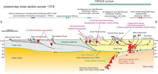
Schematic N-S cross-section of the India-Asia collision zone with speculative deep exploration along about 73°E integrating the findings of this paper with the interpreted geological evolution. The relatively low velocity crust underneath the southern part of the TIPAGE profile is correlated with shortened, thickened and warm Asian crust. It is currently ejected southward along a north-dipping Moho und buckled into large-scale crustal domes. The northern Pamir shows steep underthrusting of colder Tien Shan crust along the Main Pamir fault zone with its leading edge marked by the Moho trough beneath Lake Karakul; the Asian mantle is detached from the crust and subducts along a south-dipping Moho. Most of the Pamir is underlain by relatively cool Indian lithospheric mantle, whose leading edge is marked by the Pamir seismic zone; the Indian mantle is again detached from the crust. The horizontal line within the Asian crust marks the position of the boundary between the upper and lower crust derived in this study. Red dots mark main earthquakes of the Pamir seismic zone and the crustal seismicity along the Main Pamir fault zone plotted along section T-T' of Pegler and Das (1998). Black dots mark the Moho data of Beloussov et al. (1980); the blue line is the Moho interpreted from this study. The upper two panels of the figure put the present-day cross-sectional features into the geological history. Shortening estimates and time frames of the Pamir part of the sections are from unpublished results of the TIPAGE group; those from the Himalayas and the Kohistan-Ladakh arc are from lithosphere-scale considerations (Negredo et al. 2007) and interpretations of the geological record, recently summarized by Yin (2006). The ages of the Tirich Mir and Baltoro leucogranites are from Parrish and Tirrul (1989), Fraser et al. (2001) and Hildebrand et al. (1998, 2001).
The type of Moho structure found in this study can be compared to that found in other continent-continent orogens other than the Himalaya-Tibet system, for example the Alps and the Urals. Compared to the Pamir, the Alps are an extremely well-studied orogenic belt from the point of view of high-resolution, controlled-source seismology. Not only can a well-developed crustal root up to 20 km thick beneath the mountain belt be recognized, but on three N-S seismic transects resulting from the EGT, TRANSALP and ALP2002 projects, spanning an along-strike distance of about 300 km, it can be seen that the northern European plate underthrusts the southern Adriatic microplate at the level of the Moho (Ye et al. 1995; TRANSALP Working Group 2002; Bleibinhaus & Gebrande 2006; Lüschen et al. 2006; Brückl et al. 2007). In the case of the Urals, the Palaeozoic mountain belt marking the boundary between the East European Craton to the west and the Asian collage of terranes to the east, a 10-15-km-thick crustal root has also been identified from controlled-source seismic studies (Carbonell et al. 1996; Knapp et al. 1996; Stadtlander et al. 1999; Kashubin et al. 2009). In the middle Urals there is evidence from seismic data that the western East European Craton has been underthrust by the eastern West Siberian plate (Kashubin et al. 2006, 2009), whereas in the southern Urals the picture is less clear. Many other Palaeozoic orogens, for example the Variscides, Caledonides and Appalachians have no crustal root anymore, due to post-orogenic extension and re-equilibration of the lithosphere (Berzin et al. 1996). The shape of the Moho presented in this study shows most similarity to that of the southern Urals (Carbonell et al. 1996; Stadtlander et al. 1999), although this picture may change somewhat if and when high-quality, deep-crustal seismic data from controlled-source experiments become available.
The value for the average uppermost mantle velocity sampled by the Pn phase of 8.10-8.15 km s-1 is close to the global average value of 8.09 ± 0.20 km s-1 but is somewhat higher than the global value for orogens of 8.01 ± 0.22 km s-1 (Christensen & Mooney 1995). Taking into account the ellipticity of the Earth and assuming that the uppermost mantle beneath the profile is essentially isotropic, indicates relatively cool uppermost mantle temperatures of 700-800°C beneath the profile. In deriving these temperatures, the method of Hacker & Abers (2004) was used to calculate the velocities of common mantle compositions. These relatively cool temperatures would in turn indicate an intact mantle lid beneath the profile. Alternatively, if the uppermost mantle beneath the profile is significantly anisotropic, then the value of 8.10-8.15 km s-1 could indicate that the fast direction of the anisotropic material is close to being oriented along the profile.
Using P-wave tomographic imaging, Li et al. (2008) showed that the distance over which presumed (continental) Indian lithosphere has thrust under Tibet decreases from west, where it probably underlies most of the plateau, to east, where it extends no further than the Yarlung-Tsangpo suture zone. Kumar et al. (2006) and Jiménez-Munt et al. (2008) suggested that about 500 km of Indian lithosphere is ‘subducting’ beneath the central Tibet plateau almost horizontally. Fig. 13 integrates the findings of this study in a schematic lithosphere-scale cross-section of the India-Asia collision zone at about 73°E. The Hindu Kush seismic zone which dips northward at about 80° is to the west and only the Pamir seismic zone crosses the section. Indian crust subducts almost horizontally and is replaced beneath the southernmost Pamir by Asian crust that is currently ejected southward along a north-dipping Moho und buckled into large-scale crustal domes. Indian mantle lithosphere extends further north suggesting that the half-arc-shaped Pamir seismic zone outlines its northwestern leading edge. This Indian mantle lithosphere could correspond to the cool upper mantle derived in this study. The Asian crust shows significant increase in N-S shortening and vertical thickening from the Tien Shan to the Pamir, attaining high crustal temperatures with migmatization and leucogranite injection from the central Pamir southward. The northern Pamir may record steep underthrusting of colder Tien Shan crust, equivalent to the crust beneath the Tarim and Tajik basins, along the Main Pamir fault with its leading edge marked by the Moho trough beneath Lake Karakul. The leading edge is likely outlined by the seismically most active part of the crust in the Pamir (e.g. Pegler & Das 1998). The Asian mantle is detached from the crust and subducts along a south-dipping Moho. If, and to what extent, the mantle reflector identified in this study has anything to do with the North Pamir seismic zone (Fig. 13) remains the subject of further study on this zone.
In summary, using 11 well-located, approximately in-line earthquakes, it has been possible to construct 2-D P- and S-velocity models along the main profile of the TIPAGE project array, based on seismic refraction/wide-angle reflection observations. Crustal thickness increases from about 65.5 km close to the southern end of the profile to about 73.6 km, 10 km south of the middle of the profile under Lake Karakul in the northern Pamir. It then decreases again to about 57.7 km, 50 km south of the northern end of the profile beneath the southern Tien Shan. The main upper crustal layer which extends down to about 27 km b.s.l. has average P velocities of 6.05-6.1 km s-1 and a Poisson′s ratio (σ) of 0.26 except beneath the south central part of the profile. Here, beneath the central Pamir, the average P velocity decreases to 5.95 km s-1 and Poisson′s ratio (σ) is as low as 0.22. This is similar to the situation in central Tibet (Mechie et al. 2004) and is indicative of felsic rocks rich in quartz in the a state (Sobolev & Babeyko 1994; Christensen 1996). Below the rest of the profile a granodioritic composition for this layer is indicated (Christensen 1996). The lower crust has P velocities varying from about 6.1 km s-1 at the top to about 7.1 km s-1 at the base. It has a σ of 0.27-0.28 towards the northern end of the profile. In contrast, beneath the central and southern parts of the profile, the lower crust exhibits a low σ of 0.24 which is similar to values found in the northeast Tibetan plateau (Galvé 2006; Jiang et al. 2006). The velocities and low σ under the southern and central parts of the profile can be explained by felsic schists and gneisses in the upper part of the lower crust transitioning to granulite-facies and possibly also eclogite-facies metapelites in the lower part (Holbrook et al. 1992; Lutkov 2003; Hacker et al. 2005; Gordon et al. 2011). Assuming a more or less isotropic uppermost mantle, the average P velocity of 8.10-8.15 km s-1 indicates relatively cool uppermost mantle temperatures of 700-800°C beneath the profile which, in turn would indicate the existence of an intact mantle lid beneath the profile. The preferred model from this study for the crustal and lithospheric mantle structure beneath the Pamir is an almost horizontal underthrusting of relatively cool Indian mantle lithosphere up to the central Pamir overlain by thick, warm Asian crust. Comparison with Tibet and other orogens reveals many similarities, especially beneath the southern part of the profile below the Pamir, for example large crustal thickness and a crustal root, low average crustal P velocity, and low Poisson′s ratio in both the upper and lower crust. In contrast to central and eastern Tibet but similar to western Tibet, Indian mantle lithosphere reaches far to the north in the Pamir underlying most of the plateau. Nevertheless, in order to reveal more details of the crustal structure of this region, for example the detailed structure of the top 5 km including detailed mapping of the top of the seismic basement, details of the boundary between the upper and lower crust including better depth constraints, and the possible identification of the a-β quartz transition, new controlled-source seismic experiments are required in the region.
Acknowledgments
The TIPAGE project is funded by the Deutsches GeoForschungsZentrum-GFZ, Potsdam and the Deutsche Forschungsgemeinschaft (bundle 443, projects RI1127/8, RA442/34). The instruments used in the field program were provided by the Geophysical Instrument Pool of the Deutsches GeoForschungsZentrum-GFZ, Potsdam and the German Task Force for Earthquakes also at the Deutsches GeoForschungsZentrum-GFZ, Potsdam. M. Sobesiak is acknowledged for organizing the German Task Force mission to the Kyrgyz Republic following the Mw= 6.6 Nura earthquake of 2008 October 5 and S. Eggert is acknowledged for helping with deployment of the German Task Force stations. The data for the station OHH were obtained from the Incorporated Research Institutions for Seismology (IRIS) data management centre. Station OHH belongs to the Kyrgyz Digital Network, run by the Institute of Seismology of the National Academy of Sciences of the Kyrgyz Republic (NAS KR KIS). Fig. 13 received valuable input from B.R. Hacker (UCSB). Many of the figures were prepared with the help of the GMT plotting routines (Wessel & Smith 1991).
References
