Teleseismic tomography of the mantle in the Carpathian-Pannonian region of central Europe Free

Summary

1 Introduction

1.1 Background

The Carpathian–Pannonian system is one of the key structural features of the European continent and has been intensively studied over the past three decades (e.g. Royden et al. 1983a; Horváth 1993). The present structure of the Carpathian–Pannonian system (Fig. 1) is the result of Cretaceous to Miocene convergence as the European plate collided with a series of continental fragments to the south and the Tethys Ocean closed (Ustaszewski et al. 2008). Anticlockwise rotation and northward indentation of the Adriatic microplate produced lateral extrusion of an East Alpine block, uplift of the Carpathians and eastward extension of the Pannonian Basin until the mid-Miocene. Several hypotheses have been proposed to explain the uplift of the Carpathians and the extension of the Pannonian Basin. These include extension driven by a mantle plume or upwelling (e.g. Stegena et al. 1975; Huismans et al. 2001), subduction and roll-back along the Eastern Carpathian margin (e.g. Royden et al. 1983a; Horváth 1993), mantle flow due to escape tectonics from the Alpine collision (Kovács & Szabó 2008) and gravitational instability of the lithospheric mantle producing synchronous convergence in the Carpathians, and thinning of the lithosphere in the basin (Houseman & Gemmer 2007).

Figure 1

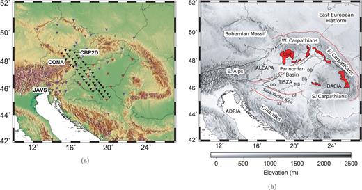
(a) Distribution of broad-band stations used in the study. Purple triangles are the permanent seismological stations, black triangles the Carpathian Basins Project (CBP) 30 s period instruments, red triangles the CBP 100 s period instruments. The locations of three stations used in Fig. 5 are shown; (b) Sketch map of the Carpathian–Pannonian region. Simplified surface structural features are shown as black and red lines. The Middle Miocene to subrecent magmatic rock outcrops after Kovács et al. (2007) are shown in red. Abbreviations show features referred to in the text: MHL, Mid-Hungarian Line; PKB, Pieniny Klippen Belt; PAL, Periadriatic Line; DF, Drava Fault; SF, Sava Fault; DD, Drava depression; MB, Makó basin; BB, Békés basin; DB, Derecske basin; CSVF, Central Slovakian volcanic field.

Open in new tabDownload slide

To provide additional control on models for the formation of the Pannonian Basin, we deployed in the Carpathian Basins Project (CBP) a temporary seismological network, consisting of 56 broad-band seismometers, across Austria, Hungary and Serbia (Fig. 1) for 16 months in 2006–2007. Together, with data from a further 44 permanent stations we have imaged the upper-mantle velocity structure down to depths of 850 km by inversion of P- and S-wave teleseismic traveltime residuals. This data set enables new regional-scale tomographic images of the mantle beneath the Pannonian Basin and adjacent Carpathian mountain belt. The spatial resolution of these new images is significantly improved on earlier tomographic solutions (Wortel & Spakman 2000; Piromallo & Morelli 2003; Koulakov et al. 2009; Chang et al. 2010), allowing new insights into the processes that produced the basin.

1.2 Tectonic setting

The uplift of the Carpathians, Eastern Alps and Dinarides, which surround the Pannonian Basin, began in the Cretaceous as a result of collision between the Adriatic microplate and the European continent (Royden et al. 1982). The inner Carpathian region consists of two microplates: an Eastern Alpine, Alcapa terrain, which was extruded from the Late Eocene (Csontos et al. 1992) along the Pieniny Klippen Belt to the north and the Mid-Hungarian shear zone to the south (Fig. 1), and the Tisza-Dacia terrain, which was extruded at a slower rate, causing dextral shearing along the Mid-Hungarian shear zone (Márton & Fodor 1995). The extrusion was accompanied by extension and anticlockwise rotation of Alcapa and clockwise rotation of Tisza-Dacia (Csontos & Nagymarosy 1998).

The lithospheric extension and mantle upwelling of a previously thickened crust and lithosphere (Stegena et al. 1975) occurred from the Mid to Late Miocene (Horváth 1995), to form the Pannonian Basin. The basin consists of a set of small, deep subbasins, separated by relatively shallow basement blocks; the Neogene-Quaternary sediments, in some of these subbasins, exceed 7 km in thickness (Kilényi et al. 1991). In the northern part of the Pannonian Basin and in the East Carpathians (Fig. 1), Miocene calcalkaline volcanics, thought by some to be related to backarc spreading and eastward retreat of a subduction zone, occurred at the same time as underthrusting in the Carpathian mountains and basin subsidence in the Pannonian region (Lexa & Konečný 1998). Later, alkaline basalts erupted in the Pannonian Basin itself, due to the extension and asthenospheric up-doming. Heat flow, in the Palaeozoic domains north of the Carpathians, is between 40–70 mW m⁻², with even higher values (80–110 mW m⁻²) in the Pannonian Basin (Tari et al. 1999).

The present-day compressive stress field, observed within the Pannonian Basin, is thought to be the result of the continued convergence of the Adriatic microplate and the European plate by about 3 mm yr⁻¹(Grenerczy & Kenyeres 2006), causing inversion of pre-existing extensional faults and reactivation of shear zones (e.g. Gerner et al. 1999; Bada et al. 2007).

An early model for the development of the Pannonian Basin inferred the presence of a mantle diapir, which eroded the base of the crust (Stegena et al. 1975); active mantle upwelling has also been proposed more recently by Huismans et al. (2001). The most commonly cited driving force behind extension is the subduction of oceanic lithosphere along the Carpathian margin and slab roll-back, which resulted in asthenospheric upwelling and rifting (e.g. Horváth 1993; Wortel & Spakman 2000). In this model extension finally ended with the complete consumption of oceanic lithosphere, followed by slab detachment and a gradual increase in horizontal compressive stress in the Neogene (Horváth et al. 2006; Bada et al. 2007). The slab roll-back model has dominated structural and geological interpretations of this region in recent decades, but alternative ideas have been proposed: Kovács & Szabó (2008) challenged the presence of a subduction margin along the Western Carpathians and explained the extension by mantle flow associated with eastward extrusion from the Alpine compression; Houseman & Gemmer (2007) proposed a model where collapse of overthickened continental lithosphere triggered the development of gravitational downwelling of the mantle lithosphere beneath the Carpathians and synchronous extension of the Pannonian Basin.

1.3 Previous seismological work

Since 1997, central Europe has been covered extensively by controlled-source refraction and wide-angle reflection seismic experiments (Guterch et al. 2003) and, together with receiver function analyses (e.g. Diehl et al. 2005; Hétenyi & Bus 2007; Geissler et al. 2008), the crustal structure is reasonably well known. Crustal thickness varies between 24–30 km in the Pannonian Basin, 29–37 km in the Western Carpathians, up to 43 km beneath the SE Carpathians, 31–48 km in the Eastern Alps, 39 km in the Dinarides and up to 38 km in the Bohemian Massif (Grad et al. 2009). There are also strong lateral crustal changes between the crust of the European plate, the Adriatic microplate and the Pannonian domain at the western boundary of the Pannonian Basin (Brückl et al. 2003; Behm et al. 2007a). Across the Western Carpathians, on the northern boundary of the Pannonian Basin, Środa (2010) interprets the results of crustal seismic surveys in terms of underthrusting and delamination of Alcapa continental lithosphere.

Using teleseismic P-wave relative arrival-time residuals, Babuška et al. (1987) and Babuška & Plomerová (1988) produced the first model of lithospheric thickness in the Carpathian–Pannonian region, which has since been developed with further geophysical data sets (e.g. Horváth 1993; Posgay et al. 1995; Ádám 1996; Zeyen et al. 2002; Horváth et al. 2006). Lithospheric thicknesses vary from around 50 km in the basin to 140 km or more beneath the East European platform.

Wortel & Spakman (2000) used regional tomography to image slow seismic velocities in the upper mantle for the Pannonian region, with fast seismic velocities in the mantle transition zone (MTZ). The latter was interpreted as the result of subduction of oceanic material along the Carpathian margin since 16 Ma, and the progressive detachment of an east Carpathian slab starting at ca. 10 Ma in the north and culminating today beneath the SE Carpathian region of Vrancea. Piromallo & Morelli (2003) obtained better resolved images in their tomographic study of the Alpine–Mediterranean region and also imaged fast velocities within the MTZ beneath southern and central Europe, which they interpreted as remnant Tethyan oceanic lithosphere. In an S-wave study, using both body and surface waves, Chang et al. (2010) inferred hot upwelling mantle in the top 200 km under the Pannonian Basin from the low asthenospheric velocities.

Receiver functions have also been used to determine the depth and thickness of the MTZ beneath the Carpathian–Pannonian region (Hetényi et al. 2009) and the greater Alpine region (Lombardi et al. 2009). These studies show a relatively flat 410 km discontinuity with a depression of the 660 km discontinuity by up to 40 km under the Pannonian Basin and the Alps. The thickened MTZ is indicative of cold, dense material within the transition zone, consistent with the higher velocities imaged by tomography (e.g. Wortel & Spakman 2000; Piromallo & Morelli 2003).

2 Data

The temporary network deployed as part of the CBP consisted of 46 CMG-6TD (30 s period) sensors spaced at approximately 30 km intervals along three ∼450 km profiles through eastern Austria, western Hungary and northern Serbia; 10 CMG-3T(D) (120 s period) sensors were also deployed throughout the Pannonian Basin in Hungary, Croatia and Serbia (Fig. 1). Most instruments recorded at 100 sps; several at 50 sps. The CMG-6TD sensors were operational for 16 months from 2006 May to 2007 August; the CMG-3T(D) sensors were deployed for 24 months from 2005 October. The CMG-6TD network was designed to cross the Mid-Hungarian shear zone, the boundary between the Alcapa and Tisza–Dacia terrains and a major structural feature of the Pannonian Basin. To supplement the CBP data, teleseismic earthquake records were collected from 44 permanent broad-band stations in the Pannonian–Carpathian region (Fig. 1) for the 16-month period that the CBP network was fully operational.

The Bulletin of the International Seismological Centre was searched for earthquakes with M_w > 5.5 in the distance range from 30° to 100° from the centre of the CBP network for the 16 months after 2006 May. After bandpassing the data with a Butterworth zero-phase, two-pole filter (0.4–2 Hz for P waves; 0.04–0.1 Hz for S waves), all seismograms were visually inspected; only those earthquakes, which had good signal-to-noise waveforms on at least 30 stations, were selected for further analysis. The final data set, from up to 100 seismic stations, consisted of 15 853 P-wave arrival-time measurements from 225 earthquakes and 8016 S-wave arrival-times from 124 earthquakes (Fig. 2). Absolute arrival-time residuals (Dando 2010) determined relative to iasp91 (Kennett & Engdahl 1991) for the P-wave data set (15 853 rays) show a regional fast mean residual of −1.46 s with an rms variation of 1.82 s.

Figure 2

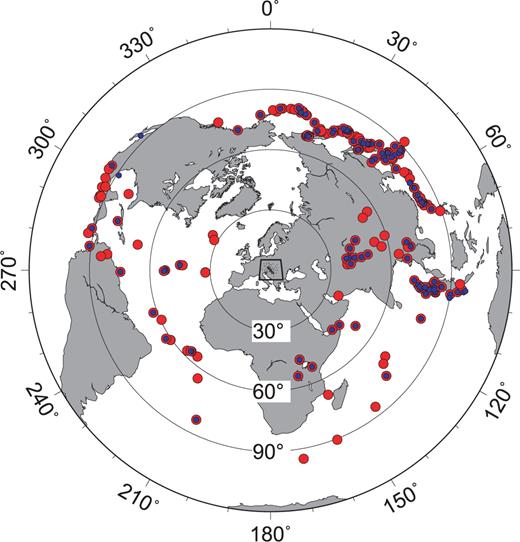
Azimuthal projection of the earthquake epicentres recorded from 2006 May to 2007 August used in the tomographic inversion. Red circles show the 225 earthquakes used in the P-wave inversion; smaller blue circles show the 124 events used in the S-wave inversion. 30° distance increments are marked from the centre of the CBP network.

Open in new tabDownload slide

3 Relative Arrival Time Residuals

We use relative rather than absolute arrival-time residuals in our tomographic inversion to mitigate source errors and the effects of mantle heterogeneity outside the model volume. The relative-arrival times are determined using the multichannel cross correlation (MCCC) technique (VanDecar & Crosson 1990) using a 3 s window for the P waves and a 30 s window for S waves. The technique requires an initial estimate of the arrival time, for which we used the adaptive stacking technique of Rawlinson & Kennett (2004), manually picking the stacked trace at the first dominant peak or trough. The time-shifts required to align each station waveform with the stacked trace then provided an initial estimate for the MCCC technique.

The relative arrival-time residual for each station (t_RESi) is given by the difference between the arrival time at each station (t_i) and the theoretical iasp91 arrival time, t_iaspi with the mean residual for each event () removed.

1

3.1 Assessing the quality of the relative arrival-time residuals

Possible sources of error in the relative arrival-time residuals include cycle skipping, noisy waveforms and timing errors. To remove cycle skipped data, all traces were visually inspected after applying the MCCC-derived time-shifts. Noisy traces with an average MCCC correlation coefficient (VanDecar & Crosson 1990) of less than 0.79 were removed. Residuals that differed within a 10° backazimuth bin by more than 2 standard deviations from the median residual in any station set were also removed. The MCCC was then rerun, resulting in a set of residuals, self-consistent for each station.

We estimated the relative arrival-time residual error by comparing earthquakes with hypocentres close to one another. From a cluster of eight Kuril Islands earthquakes (M_w 5.5 to M_w 7.9) with epicentres within 46 km of each other, the standard deviation of the relative arrival-time residuals was obtained at each of the 100 stations. The average of these standard deviations is 0.040 s (with a range from 0.01 s to 0.07 s) for P waves and 0.313 s (with a range from 0.021 s to 0.944 s) for S waves; these uncertainty estimates are comparable with those from similar tomographic studies (e.g. Tilmann et al. 2001).

3.2 Observed relative arrival-time residuals

Fig. 3 shows the mean relative P-wave arrival-time residuals across the Carpathian–Pannonian system for ray paths propagating from the north, east, southwest and west. For ray paths from the north (Fig. 3a), early arrivals dominate south of the Mid-Hungarian shear zone in the Tisza-Dacia domain, north and south of the Eastern Alps and in the east. This signature reflects deep-sourced fast anomalies below the Bohemian Massif, the Eastern Alps and to the east beneath the Pannonian Basin and Eastern Carpathians. Arrivals from the east (Fig. 3b) produce a broadly consistent picture, though the residuals are decreased in amplitude across the basin. From the southwest and the west (Figs 3c and d), the pattern of residuals across the basin is now reversed; higher velocities under the Alps advance the arrivals observed at stations in the Vienna Basin and the Alcapa block. The equivalent S-wave residuals have a similar geometric distribution, but about twice the amplitude. The observed median P-wave relative arrival-time residuals vary between −1.13 s (early) in the Alps to 1.12 s (late) at the western end of the Carpathians; S-wave relative arrival-time residuals are about twice as large (−2.13 s to 3.39 s).

Figure 3

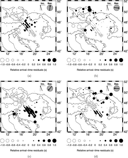
Mean P-wave relative arrival-time residuals (positive is delayed) recorded from four source regions. Average backazimuth and near-surface inclination are shown. Station terms have been removed from the data. (a) From the north (22 events); (b) from the east (30 events); (c) from the southwest (7 events) and (d) from the west (22 events).

Open in new tabDownload slide

4 Inversion Method and Model Parametrization

The relationship between the traveltime and slowness along a path is non-linear, since the path depends on the slowness field. However, for small slowness perturbations in the model, Fermat's Principle allows for a first-order linear relationship between traveltime perturbations and slowness perturbations,

2

that is, the traveltime perturbation Δt_i is calculated by integrating the slowness perturbations Δs(r) along the ray path L^ref_i in the model.

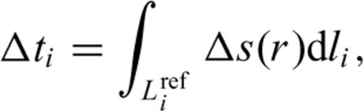
The relative arrival-time residuals were inverted for slowness perturbations using the method of VanDecar et al. (1995). The P-wave slowness field is parametrized using a set of smoothly varying cubic splines under tension, relative to a spherically symmetric background model (iasp91). The splines are locally constrained by a 3-D grid of nodes. In depth, our grid consists of 35 nodes spaced at 25 km intervals between 0 and 850 km; at each level the the grid consists of 60 nodes in latitude, spaced at intervals of 0.25° from 39.75° to 54.5°, and 99 nodes in longitude at intervals of 0.25°, from 6° to 30.5°. With the network aperture reaching 888 km, we have separately tested grids that extend to depths of between 700 km and 1000 km (Dando 2010). A depth extent of 700 km results in truncation of the deepest anomalies at the base of the model, distorting the image. We chose to use 850 km as the base of the inversion solution, as the inversion images change little when the base is moved to 1000 km depth and the residual reduction changes by less than 0.005 per cent.

The inversion simultaneously solves for slowness perturbations and arrival-time correction terms associated with individual sources and stations (VanDecar et al. 1995). Source adjustment terms are included to account for small variations in the backazimuth or angles of incidence caused by the hypocentral error, as well as velocity heterogeneities external to the grid. The station terms take into account traveltime anomalies associated with the crust and uppermost mantle directly beneath each receiver; a general lack of crossing rays at shallow depths prevents resolution of vertical structure in this region and using station terms avoids surficial features being mapped into the mantle model. The typical minimum station spacing is 30 km beneath the densely sampled part of the CBP array, but elsewhere it can be sparse—42 km on average; we therefore do not interpret velocity anomalies above 75 km.

As there are more unknowns (P waves 20 8900; S waves 20 8495) than observations (P waves 15 853; S waves 8016), our inverse problem is underdetermined and regularization is required to find a unique solution. We choose regularization parameters which deliver a model that contains the least amount of structure consistent with the data (e.g. Constable et al. 1987; VanDecar 1991). The boundary nodes are heavily damped such that the 3-D model merges smoothly into the surrounding radially symmetric iasp91 reference earth model. In addition, the model is regularized in terms of smoothing and flattening parameters to suppress, respectively, the curvature of the model (∇²s) and the spatial gradient (∇s) of the solution. The ratio of the two regularization parameters was chosen so that both smoothing and flattening terms had similar impact on model roughness.

We investigated the trade-off between data misfit and the model roughness, using a finite difference approximation to the Laplacian operator, to select a preferred model that fits the data without introducing evident noise. The final choice of the regularization parameters was based on the comparison of inversion solutions shown in relation to the trade-off curve as shown for the P-wave inversions in Fig. 4. The preferred choice provides a smooth model while still containing plausible short-wavelength structure as revealed in resolution tests. The resulting P-wave model produces a 71 per cent reduction of the rms residual from 0.446 s to 0.130 s. The effect of station terms alone reduces the P-wave rms residual from the initial 0.446 s to 0.365 s. For the S-wave model, the rms residual was reduced from 1.513 s to 0.624 s. The effect of station terms alone, reduces the initial S-wave rms residual from 1.513 s to 1.317 s.

Figure 4

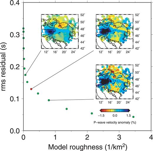
Trade-off between the model roughness and rms residual for the P-wave inversions. The three images show the 300 km depth slice for three different sets of regularization parameters. The red point shows the preferred model solution using smoothing parameter λ_s = 14 000 and flattening parameter λ_f= 750.

Open in new tabDownload slide

The remaining residuals have been examined both on a station-by-station basis and event-by-event basis to identify any systematic trends in the remaining misfit. Fig. 5 shows the residuals for three typical stations. The residuals have been reduced to near-zero and show no further systematic misfit with respect to distance and backazimuth. The forward model calculation adequately represents the dependence of arrival-time residual on backazimuth seen in the observed data.

Figure 5

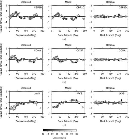
Variation of P-wave relative arrival-time residuals with backazimuth for three typical stations: CBP2D, CONA and JAVS (locations are shown in Fig. 1a). Left panel: observed relative arrival-time residuals; Middle panel: relative arrival-time residuals predicted from the solution model; Right panel: final data residuals after the inversion.

Open in new tabDownload slide

4.1 Deterministic corrections for variations in crustal structure

Although the inversion scheme includes station terms for reducing the effect of a heterogeneous and unresolved crust, a number of regional tomographic studies (e.g. Waldhauser et al. 2002; Martin et al. 2005) apply deterministic crustal corrections to the traveltime residuals using a priori knowledge of crustal velocity structure from previous geophysical studies. Waldhauser et al. (2002) show that if station terms are not used and crustal anomalies are not corrected for, erroneous structure may be mapped into the upper mantle.

We compared inversion solutions of the relative arrival-time residuals, with and without a deterministic crustal correction, and with and without station terms (Dando 2010). The crustal correction times (t_corr), were determined for individual rays relative to the iasp91 times to a reference crustal datum (H_D) of 32.2 km (the mean crustal thickness beneath all the stations), using the following formula:

3

where (t^D_iasp91) is the iasp91 time from the receiver to the datum, t^M_mod is the new crustal model time to the Moho, t^MD_iasp91 is the time from the Moho to the datum and t_topo is the traveltime associated with the station elevation. When crustal corrections were applied, average P-wave crustal velocities for this region were obtained from 3-D models determined from controlled-source experiments by Behm et al. (2007b) and Kovács (personal communication, 2009). Crustal thicknesses were obtained from the compilation of Grad et al. (2009). For 15 of the permanent stations, crustal velocities were obtained from other seismic studies (Crotwell & Owens 2005; Geissler et al. 2008).

Applying the crustal corrections to the raw P-wave residuals reduces the rms residual from 0.446 s to 0.438 s (Figs 6a and b). If station terms are not used, the post-inversion rms residual decreases from 0.154 s to 0.149 s (Figs 6c and d) when the crustal corrections are applied. When station terms are solved for, the post-inversion rms residual is 0.130 s without the crustal correction (Fig. 6e) and 0.131 s with the crustal correction (Fig. 6f), with no significant changes in the tomographic images in these two cases. The deterministic crustal corrections therefore produce a model which accounts for slightly more of the data compared with no correction, but station terms are still necessary. When crustal corrections are applied, the rms station term is reduced from 0.243 s to 0.229 s (Fig. 7). While the crustal corrections are only as good as the crustal model, we conclude that the station terms derived from the VanDecar et al. (1995) inversion provide a robust method of accounting for near-surface traveltime variations which are not constrained by crossing ray paths in the tomographic inversion. The deterministic corrections only account for approximately 6 per cent of such variations; the other 94 per cent appear to require significant velocity variation in the uppermost mantle, or crustal structure that is not recognized in the deterministic corrections. Effects of including these corrections or the station terms on the model solution are minor and limited to the upper 150 km (Dando 2010). The station terms showed no correlation with region but revealed three P-wave station terms of about 1 s, anomalous compared to the surrounding stations; these anomalies are attributed to leap-second errors in the recording equipment which are captured in the station terms.

Figure 6

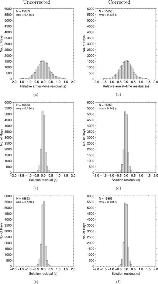
Histograms of the P-wave relative arrival-time residuals both without (left-hand side) and with (right-hand side) deterministic crustal corrections. The observed relative arrival-time residuals are shown in (a) and (b). The residuals after tomographic inversion are shown without station terms (c and d) and with station terms (e and f).

Open in new tabDownload slide

Figure 7

Distribution of station terms for inversions without (a) and with (b) the deterministic crustal correction applied to the raw P-wave residuals. The histograms show a reduction in the rms from 0.243 s to 0.229 s with the correction applied.

Open in new tabDownload slide

5 Results

5.1 Checkerboard tests

With near-vertical ray paths, teleseismic tomography is relatively good at resolving lateral velocity variations, but tends to blur velocity anomalies in the vertical direction. We investigate the robustness of the tomographic images using checkerboard tests and a synthetic model based on simple geometric shapes relevant to our solution for the P-wave inversion. Forward traveltimes are calculated using the same set of source–receiver paths as our data set, and are inverted using the same model parametrization and regularization. To simulate measurement error, Gaussian noise with a standard deviation of 0.040 s and 0.313 s, as estimated, respectively, for the P- and S-wave relative arrival-time uncertainty, is added to the synthetic traveltimes.

The checkerboard models consist of alternating positive and negative spherical slowness anomalies (peak amplitudes of ±3 per cent in the P-wave model and ±5 per cent for S-wave model), spaced every 2° in latitude and longitude, and centred at depths of 100 km, 300 km, 500 km and 700 km (Figs 8 and 9). Each anomaly has a Gaussian decrease in amplitude from its centre (a factor of e decrease in 45 km). The checkerboard approach allows us to assess the quality of our solution model by highlighting areas of good lateral resolution and the extent to which smearing of anomalies is a problem in either horizontal or vertical directions. Figs 8 and 9 compare the recovered velocity structure with the input checkerboard model, using both vertical sections and depth slices.

Figure 8

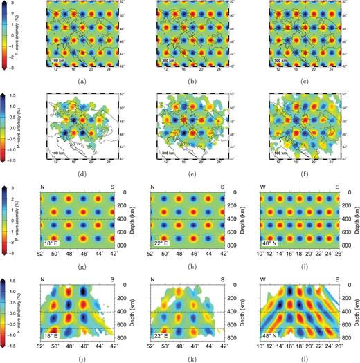
Synthetic P-wave checkerboard model. The input synthetic model is shown for three depth slices (a)–(c) and three vertical sections (g)–(i). The locations of the three vertical sections are shown in (c). The corresponding images from the inversion of the synthetic data are shown below the respective input model images. The normalized correlation between input and recovered model for the depth slices are 0.87, 0.90, 0.90 and 0.91 for 100 km, 300 km, 500 km and 700 km (not shown), respectively; for the vertical sections the correlation is 0.87 at 18°E, 0.88 at 22°E and 0.82 at 48°N. Note that the colour scales used for input and output models differ as the inversion method recovers only about half of the original anomaly amplitude.

Open in new tabDownload slide

Figure 9

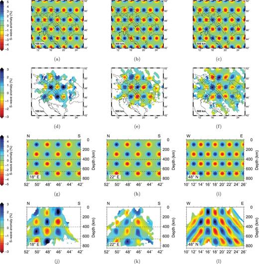
Synthetic S-wave checkerboard model. The input synthetic model is shown for three depth slices (a)–(c) and three vertical sections (g)–(i). The locations of the three vertical sections are shown in Fig. 8(c). The corresponding images from the inversion of the synthetic data are shown below the respective input model images. The normalized correlation between input and recovered model for the depth slices are 0.75, 0.89, 0.84, 0.77 for 100 km, 300 km, 500 km and 700 km (not shown), respectively; for the vertical sections the correlation is 0.83 at 18°E, 0.77 at 22°E and 0.77 at 48°N. Note that the colour scales used for input and output models differ as the inversion method recovers only about half of the original anomaly amplitude.

Open in new tabDownload slide

In general, the recovered P-wave checkerboard model (Fig. 8) shows that horizontal variation on the 50 km to 100 km length scale is adequately resolved in all regions where we have adequate ray coverage (the solution is blanked out where there are fewer than five rays intersecting an area element spanned by four nearest neighbour nodes), and the area that has good ray coverage increases systematically with depth. In the S-wave checkerboard model (Fig. 9), where ray coverage is less and the seismic wavelength may approach the diameter of the input anomaly, resolution is decreased. However, the anomalies are still resolvable on the 100 km length scale. With regularization imposed on the inversion, the peak amplitudes of the recovered anomalies are reduced by up to a factor of 2 or 3, and their radius increased correspondingly relative to the input model. Some distortion of the shape of the anomalies is also apparent, with vertical smearing evident, particularly in the east–west section where diagonally adjacent anomalies are not clearly separated (Figs 8l and 9l). In general, however, local extrema in the amplitudes of the recovered slowness field reveal the locations of the original anomalies.

5.2 Upper-mantle tomographic images

The tomographic inversion shows contrasts in the seismic velocity structure, relative to the spherically symmetric iasp91 model. The tomographic solutions are shown in Figs 10 and 11 for the P-wave images, and Figs 12 and 13 for the S-wave images. We use the descriptive terms fast and slow to refer to parts of the solution region that have seismic wave velocity that is, respectively, greater or lesser than the assumed iasp91 velocity profile. We note, however, that the actual horizontally averaged velocity profile is poorly constrained by the use of relative arrival-time residuals. Therefore the velocity anomalies we present are relative rather than absolute.

Figure 10

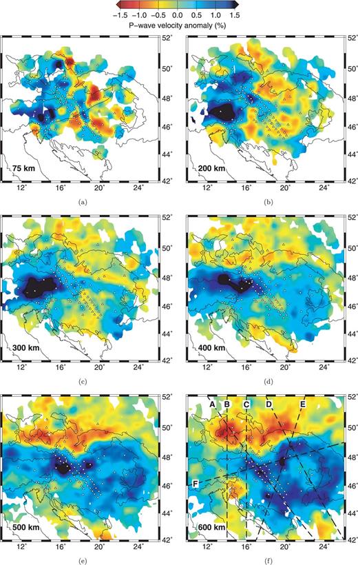
Depth slices through the P-wave tomographic model. The locations of stations are shown as triangles. Locations of vertical sections are shown on the 600 km slice. The Mid-Hungarian Line is also shown in (a) for reference. The solution is blanked out where ray coverage is inadequate.

Open in new tabDownload slide

Figure 11

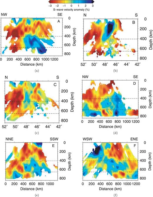
Vertical sections through the P-wave tomographic model. Locations of vertical sections are shown in Fig. 10(f). The ‘410’ and ‘660’ discontinuities are shown for reference.

Open in new tabDownload slide

Figure 12

Depth slices through the S-wave tomographic model. The locations of stations are shown as triangles. Locations of vertical sections are shown on the 600 km slice. The Mid-Hungarian Line is shown in (a) for reference.

Open in new tabDownload slide

Figure 13

Vertical sections through the S-wave tomographic model. Locations of vertical sections are shown in Fig. 12(f). The ‘410’ and ‘660’ discontinuities are shown for reference.

Open in new tabDownload slide

The lithosphere–asthenosphere boundary (LAB) is estimated to be between 45 and 60 km deep (Tari et al. 1999) beneath the Pannonian Basin. At 75 km depth, just below the LAB, we image (Fig. 10a) four localized P-wave low-velocity anomalies (< −1.66 per cent) in the upper mantle beneath the basin: (i) on the northern edge of the Pannonian Basin (48°N, 19.5°E) underlying the Neogene Central Slovakian calcalkaline volcanics (Kovács & Szabó 2008), (ii) and (iii) in the eastern Pannonian Basin (47°N, 22°E and 46°N, 20.5°E), beneath the Békés, Makó and Derecske sub-basins and (iv) in the southwest of the Pannonian Basin, proximate to the Drava depression. The equivalent S-wave slice at 75 km depth (Fig. 12a) shows low-velocity anomalies which are greater in both amplitude and spatial extent; for example the S-wave anomalies underlying the Békés and Makó basins are merged and are more than twice the relative amplitude of the corresponding P-wave anomalies. The Mid-Hungarian shear zone (MHZ), dividing the Alcapa and Tisza-Dacia terrains may exert some control on the location and extent of these anomalous regions at 75 km, but the association of the MHZ with steep velocity gradients in the NW–SE direction is hardly definitive. In both P-wave and S-wave solutions the lower velocity regions extend down to at least 200 km (Figs 10b and 12b) where they have merged and decreased in amplitude to produce a subcircular low-velocity network of anomalies underlying the surface expression of the Pannonian Basin.

Also at 75 km depth, relatively high velocities (∼1.8 per cent for P wave; ∼2.9 per cent for S wave) are imaged beneath the Eastern Alps, related to the downwelling of cold lithospheric material beneath the Alpine continental collision zone (Lippitsch et al. 2003; Mitterbauer et al. 2010). These sublithospheric high velocities extend south towards the Dinarides and north under the Bohemian Massif in the P-wave image (Fig. 10a). The Bohemian Massif is also relatively fast in the S-wave image (Fig. 12a), although it is bordered to the west by a zone of lower velocities that are associated with possible asthenospheric updoming (Plomerová 2007). In both P- and S-wave images the Bohemian Massif is also bordered to the east by a zone of lower velocities.

At 200 km and 300 km depth, both P- and S-wave images (Figs 10b and c and 12b and c) are dominated by the fast anomaly beneath the Eastern Alps. Our images reveal a largely vertical high-velocity feature beneath the Eastern Alps extending out beneath the Pannonian Basin (Figs 11c and 13c). Although a major step in crustal thickness separates the Alpine and Pannonian tectonic domains (Brückl et al. 2007), we observe fast velocity anomalies extending eastwards beneath the Pannonian Basin region and down into the MTZ. Along-strike (Figs 11f and 13f) the Eastern Alpine fast anomaly appears connected to the Pannonian fast anomaly, but whereas the Alpine anomaly is strongest above the 410 km seismic discontinuity, the Pannonian anomaly is stronger in the MTZ.

The fast Alpine–Pannonian anomaly, which dominates the depth sections at 300 km and 400 km extends down into the MTZ and, at 500 km and 600 km, is clearly limited to the north by a sharp transition to relatively slow material beneath the Bohemian Massif and the West Carpathians (Figs 10e and f and 12e and f). P- and S-wave velocities decrease by around 2.2 per cent and 5.1 per cent, respectively, across this approximately E–W boundary. There is no obvious vertical continuity, however, between this prominent structure in the MTZ and the mantle above 410 km, and thus there is no clear structural connection to equally prominent surface structural features bounding the Bohemian Massif and the West Carpathians.

South of this boundary the MTZ beneath the Pannonian-Carpathian region is relatively fast in both P- and S-wave velocity maps (Figs 10e and f and 12e and f). The fastest P-wave anomalies describe a subcircular region that roughly follows the Carpathian arc. These fast velocity anomalies at 600 km appear to surround a relatively slower velocity anomaly, suggesting the shape of a doughnut. In the Discussion section we consider the impact of a depressed 660 km seismic discontinuity on our inversions, and test simple end-member models that could explain this apparent velocity structure in the MTZ.

5.3 Synthetic model resolution tests

To assess the reliability of our final inversion solutions, we apply our inversion procedure to recover a geometrically simple synthetic P-wave model which includes structures similar to those interpreted. The synthetic model shown in Figs 14(a)–(e) includes: (i) four localized slow anomalies (−3 per cent) in the depth range 50–100 km; (ii) a fast tabular vertical structure beneath the Alps (+3 per cent) in the depth range 50–350 km, which extends out beneath the Pannonian Basin in the depth range 300–410 km and (iii) an anomalously fast (+2 per cent) MTZ roughly underlying the Pannonian Basin in the depth range 410–660 km. The shape of the observed anomalies is approximately rendered by the simplified tabular blocks in this model. Synthetic traveltimes are computed using the same ray tracing algorithm used in the inversion procedure (VanDecar et al. 1995), applied to the same set of receivers and sources used in the actual data set. Random Gaussian noise with a standard deviation of 0.04 s, corresponding to that estimated for the P-wave data, was added to the synthetic relative arrival-times.

Figure 14

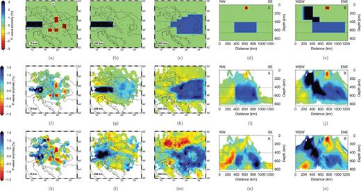
Top (a)–(e): Simplified synthetic model used to test resolution of the inversion. Middle (f)–(j): Recovered structure after the inversion of the synthetic traveltimes. Bottom (k)–(o): corresponding sections from the inversion solution of data. Locations of the vertical sections (e.g. d,e) are shown in (a). Note that the colour scales used for input and output models differ as the inversion method recovers only about half of the original anomaly amplitude.

Open in new tabDownload slide

Images recovered from inverting the synthetic traveltimes are shown in Figs 14(f)–(j), for comparison with the model recovered from the observed data (Figs 14k–o). The inversion evidently introduces some horizontal and vertical smearing, but the synthetic model structures are generally recovered wherever ray path coverage is adequate. At 75 km, the four slow anomalies are clearly imaged, although the anomaly amplitude is reduced by a factor of about 2. The apparent depth extent of the slow anomalies is approximately doubled, and the low-velocity features have fast halos in the horizontal plane. These differences should be considered when interpreting the slow-velocity anomalies seen in Fig. 10(a). The seismically fast Alpine block beneath the Eastern Alps and western Pannonian Basin is also generally well represented in the inversion images where ray coverage is adequate, though the recovered structures are vertically smeared by 50–100 km; in the central Alps recovery of the shallow fast anomaly is prevented by lack of ray coverage at lithospheric depths.

The relatively higher velocity in the MTZ is also adequately recovered, though vertical smearing increases its apparent depth extent by up to 100 km. There are minor low-velocity shadows to the north of this feature in the inverted synthetic image, but comparison with the steep velocity gradients in the real solution (Fig. 14m) shows that slower velocity material must be present to the north of the high velocity region in the MTZ. The recovered velocity anomaly at 600 km in the MTZ has the amplitude reduced by the usual factor of 2 to 3, but this image provides confidence that the central Pannonian region of apparently lower velocity at 600 km depth seen on the observed P-wave images (Fig. 14m) is well resolved and is not an artefact of the inversion.

6 Discussion

6.1 Lithospheric and upper-mantle structure

At 75 km depth, the slow anomaly beneath the northern Pannonian Basin lies beneath the Neogene volcanics of central Slovakia. This slow anomaly could be a consequence of hot mantle material that provided melt to the volcanics. This anomaly appears to extend as far south as the Mid-Hungarian Line. The other slow anomalies within the Pannonian Basin are located below three important depocentres: the Drava depression in the west, and associated with the failed Tisza rift, the Makó and Békés basins in the east (Tari et al. 1999) and the Derecske basin in the northeast (Corver et al. 2009). These low-velocity anomalies, just below the lithosphere, correlate with anomalously high heat flow [>100 mW m⁻²; Tari et al. (1999)]. Assuming that our inversion methodology and station distribution have adequately removed the effect of crustal variations on the upper-mantle solution at 75 km depth, these low-velocity anomalies presumably represent warm upwelling mantle material associated with basin extension and volcanism. Mantle lithosphere has undergone greater thinning than the crust (Royden et al. 1983b; Huismans et al. 2002) in this region and these slow anomalies could represent mantle upwellings associated with these local rift depocentres. In a recent comprehensive S-wave study of the Tethys margin, Chang et al. (2010) image low velocities down to ∼200 km depth below the Pannonian Basin; our images show these low S-wave velocities extending to greater depths (Figs 13e and f). Our P-wave inversions with better spatial resolution imply there is significant lateral heterogeneity at these depths beneath the Pannonian Basin (e.g. Fig. 10b).

Plomerová (2007) image a broad low-velocity zone down to 250 km in the western Bohemian Massif, which was interpreted either as a thermal upwelling of the LAB or the result of a deep seated mantle plume. Our solution has limited resolution in the western Bohemian massif but slow anomalies, particularly in the S-wave images are consistent with their results, although not necessarily related to the lower mantle slow anomalies of Goes et al. (1999). East of the Bohemian Massif slow anomalies are present in both P- and S-wave images and extend into the MTZ and to the east and west.

Velocity perturbations in the European upper-mantle are most likely due to temperature changes (Goes et al. 2000). Compositional variations only have a secondary effect on seismic velocity (e.g. Jackson et al. 1998; Goes et al. 2000) and are typically of the order of ±1 per cent for P waves (Cammarano et al. 2003). Goes et al. (2000) show that for a 100 °C increase in temperature, a reduction of 0.5–2 per cent in V_p and 0.7–4.5 per cent in V_s are predicted. As seen from the synthetic data tests, the recovered anomalies are typically reduced in amplitude by a factor of 2 or 3. The inferred actual amplitudes of the anomalies of about 3 per cent and 5 per cent (for P and S waves, respectively) implies that the slow anomalies are likely to be primarily thermal features. Because these anomalies are superimposed on a poorly constrained average vertical structure, however, direct interpretation of temperature variation is uncertain.

6.2 Cold downwellings in the central European upper-mantle

Fast seismic velocities are indicative of cold, higher density material, often associated with mantle downwelling. The fast anomaly we find beneath the Eastern Alps has previously been imaged using seismic tomography by Lippitsch et al. (2003). They interpreted this anomaly near 15°E as having a near-surface northeasterly dip, differing in polarity from the subduction direction further west along the Alps. Evidence of north- or south-dipping near-surface structure is equivocal in our images (Fig. 11b). Our solution shows, however, that this fast Alpine anomaly extends further east beyond the region investigated by Lippitsch et al. (2003). Below about 200 km, our images (Figs 11c and f and 13c and f) show a near-vertical fast anomaly, interpreted as a cold mantle downwelling, continuous with, but extending further east and deeper than the East Alpine anomaly. Recent work by Mitterbauer et al. (2010), based on the ALPASS data set, validates the interpretation of a relatively fast vertical structure beneath the Eastern Alps down to about 400 km.

This subvertical fast structure extends eastwards and down into a more extensive high-velocity anomaly in the MTZ beneath the Pannonian Basin. The high-velocity MTZ in this region has previously been imaged using seismic tomography (e.g. Wortel & Spakman 2000; Piromallo & Morelli 2003; Koulakov et al. 2009), but the large number of stations deployed in the CBP array has allowed us to look at this feature in new detail. Of particular interest is the relationship between the Alpine and Pannonian high-velocity anomalies, probably best seen in Figs 11(f) and 13(f). The Pannonian anomaly appears joined to the East Alpine anomaly at mid upper-mantle depths but, above 300 km it loses coherence and strength. Although this image may be affected by subvertical smearing in the E–W direction, the continuity of the structure between Alpine and Pannonian fast anomalies appears to be robust, from the synthetic test shown in Fig. 14.

Continuity of the Pannonian fast anomaly with the East Alpine fast anomaly suggests a similar origin for the relatively fast material: subvertical downwelling beneath a surface convergent zone. With this interpretation the Alpine fast anomaly is directly connected to the Alpine convergent zone which remains active, while the deeper Pannonian fast anomaly has detached from the surface and the surface convergent zone has evolved into an extensional basin. The anomalously fast regions in the transition zone beneath the SW Pannonian Basin could also be related to past subduction associated with the Vardar suture zone, but our solutions do not allow any direct links to be drawn between MTZ structures and surface features. The interpretation that emerges from our images is that a continuous collision zone extended from the Alps through present-day western and central Hungary. The apparent reduction of anomaly amplitude (e.g. Figs 11c and f and 13c and f) with depth, may reflect the structure's older origin and gradual re-equilibration with the mantle. When extension began in the Pannonian Basin, the higher velocity material detached from the lithosphere, indeed the Pannonian Basin extension may have been triggered by the detachment of this cold material produced by prior convergence. This type of event has been previously modelled in other contexts by Göğüş & Pysklywec (2008), Schott & Schmeling (1998), Davies & von Blanckenburg (1995) and Marotta et al. (1999). An alternative idea, that extension of the Pannonian Basin was driven by roll-back of a slab subducting beneath the Eastern Carpathians (Horváth 1993; Wortel & Spakman 2000) appears inconsistent with finding this anomalously fast subvertical mantle structure beneath the centre of the Pannonian Basin instead of beneath the Eastern Carpathians.

In the lower part of the MTZ beneath the eastern Pannonian Basin, the circular low-velocity region surrounded by higher velocities (the ‘doughnut’ structure imaged in Fig. 10f) also requires explanation. In vertical section (Figs 11d and 13d), the slow anomaly appears to extend beneath the 660 km discontinuity and to be enclosed above and around by a dome of higher velocity material. In the large-scale tomographic images of the region (Wortel & Spakman 2000; Piromallo & Morelli 2003), these apparently lower velocities can also be seen, albeit at lower resolution. To interpret this structure we need to take into account the effect of topography on the 660 km discontinuity. Hetényi et al. (2009), using receiver functions and a similar data set used in this study, showed deepening of the 660 km discontinuity by up to 40 km beneath the eastern Pannonian Basin, approximately beneath the centre of the ‘doughnut’ structure, whereas the 410 km discontinuity is almost flat.

We consider the low-velocity region in the centre of the ‘doughnut’ with two alternative adjustments to the synthetic model of Fig. 14. In Fig. 15(a) we remove part of the high-velocity material in the range 410–660 km to represent the case in which fast material is absent from the MTZ beneath the centre of the basin; in Fig. 15(b) we consider a locally deepened ‘660’ discontinuity. With our inversion model defined relative to the iasp91 reference earth model, P-wave velocity increases from 10.20 km s⁻¹ to 10.79 km s⁻¹ across the ‘660’ discontinuity. In Fig. 15(b) we address the effect of a 40 km depression of the ‘660’ discontinuity by adding a thin rectangular slab with velocity reduced by 3 per cent from 660 to 700 km. Comparison with the inversion solution (Figs 15g and h) shows that the second model clearly provides a reasonable explanation of the doughnut structure, consistent with the previous observations of a depressed ‘660’ and the physical model of higher velocity material downwelling beneath the centre of the basin. Depression of the 660 km discontinuity is not necessarily inconsistent with upper-mantle descending through this phase transition, but given the relatively high viscosity of the lower mantle and the relatively recent development of these tectonic events we imagine that cold upper-mantle has caused a depression of the ‘660’ without actually transferring material across it in this region.

Figure 15

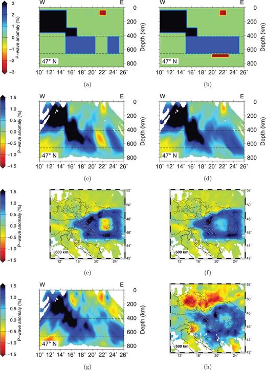
Synthetic models (a), (b) and inversion results (c)–(f) of two alternative models attempting to explain relatively low velocities in the MTZ directly beneath the Pannonian Basin: (a) with the fast anomaly removed from the MTZ, (b) with a thin rectangular slow velocity layer representing a local depression of the 660 km seismic discontinuity. E–W vertical sections (c), (d) through the centre of the Pannonian Basin and depth slices at 600 km (e), (f) are compared with the corresponding images from the actual P-wave inversion solution (g), (h). Note that the colour scales used for input and output models differ as the inversion method recovers only about half of the original anomaly amplitude.

Open in new tabDownload slide

The northern boundary of the relatively high-velocity material in the MTZ shows a sharp and well-resolved contrast with relatively low-velocity material beneath the Western Carpathians and Bohemian Massif. This boundary is proximate to the surface location of the Pieniny Klippen Belt and Penninic suture zone (Kovács et al. 2007), but the truncation of the seismic anomalies at the top of the transition zone does not enable any direct physical link to be drawn between surface and transition zone structures. We speculate instead that this boundary in the MTZ separates warm upper mantle which has been displaced northwards by the colder material that has descended into the MTZ from the Alpine–Pannonian convergent zone since the Cretaceous.

7 Conclusions

Using a 16-month temporary deployment of 56 temporary broad-band stations in the CBP network, supplemented by data from another 44 permanent stations across the Carpathian–Pannonian region, we have produced P- and S-wave tomographic images showing the upper-mantle beneath the Pannonian–Carpathian region with a resolution that has not previously been available.

The solution above 200 km reveals anomalies that are consistent with the thermal history of volcanism and the location of extensional depocentres, but we do not see a distinct velocity signature related to the Mid-Hungarian shear zone which separates the Alcapa and Tisza-Dacia blocks.

Our tomographic solution for the upper-mantle of central Europe is dominated by seismically fast anomalies arising from near-vertical lithospheric downwelling produced by the continuing convergence of Adria and Europe. Higher velocity material produced by downwelling of continental lithosphere beneath the Eastern Alps dominates the model in the upper 300 km. This high-velocity anomaly extends eastwards from the Alps beneath the Pannonian Basin, where it is attenuated above 300 km depth but clearly defined in the MTZ. Beneath the Pannonian the higher velocity material is detached from the lithosphere and is interpreted as relict downwelling of continental lithosphere from a convergent zone which pre-dated the Pannonian extension and was laterally contiguous with the Eastern Alps.

In the MTZ the entire Pannonian Basin region is underlain by higher velocity material, terminated to the north by a relatively sharp transition to relatively slow material beneath the Bohemian Massif and the West Carpathians. Within the MTZ, the fast material is disposed in a doughnut-shaped structure beneath the Carpathian arc, surrounding apparently slower material beneath the Pannonian Basin. We explain this signature as the consequence of a large mass of cold dense material depressing the 660 km seismic discontinuity beneath the cold downwelling structure described. In the MTZ the sharp transition to slower velocities north of the basin thus would represent the northern boundary of the cold material which has been spreading outwards from beneath the basin since detachment of the fast material from a Pannonian convergent zone which pre-dated Miocene extension.

Vertical cross-sections through the Western Carpathians, show no clear evidence of recent subduction or lithospheric foundering, mechanisms which have been previously suggested as possible causes for the lithospheric extension of the Pannonian Basin. If subduction beneath the Carpathians had been the main driver of Pannonian Basin extension, then the most recent downwelling should have been directly beneath the Carpathian perimeter of the basin, and there would be no reason to expect a fast anomaly stretching across the centre of the basin at 300 km depth.

Acknowledgments

The CBP was supported by a NERC standard grant (NE/C004574/1). BD undertook this work while on a NERC studentship (NER/S/J/2006/14333). The NERC Geophysical Equipment Pool (SEIS-UK) provided most of the seismological equipment used in the CBP network. Eötvös Loránd Geophysical Institute (ELGI), Technical University of Vienna (TU Wien) and the Seismological Survey of Serbia (SSS) provided extensive logistical support for fieldwork. Operations in Hungary were managed by Attila Kovács, in Austria by Helmut Hausmann. We thank also G. Falus, I. Torok, I. László, R. Csabafi, from ELGI; M. Behm (for his crustal model) and W. Loderer, from TU-Wien, V. Kovacevic, S. Petrovic and D. Valcic from SSS, and the staff of SEIS-UK (A. Brisbourne, D. Hawthorn and A. Horleston) for assistance with field operations. Additional data were provided by Geofon, the GFZ Seismological Data Archive, ORFEUS, IRIS and the Hungarian Academy of Sciences, Geodetical and Geophysical Research Institute. We thank G. Hetényi for helpful discussions, I. Bastow for comments on a draft manuscript and J. Ritter and R. England for constructive reviews. J. VanDecar and N. Rawlinson kindly provided their software. Figures were produced using GMT (Wessel & Smith 1998).

References

Author notes