Comparison of GPS strain rate computing methods and their reliability

Summary

1 Introduction

Measurements of crustal stress and strain have long persisted as hot topics in geosciences. Caporali (2003) discussed the relation between the two and the deformation property of the area of interest by analysing the GPS velocity rate and seismic mechanism solution. He also investigated the data problem and least-squares covariance matrix configuration. Hori et al. (2001) inverted for the stress field using a GPS strain field. Bayer et al. (2006) comprehensively analysed deformation in Iran based on GPS displacement and strain fields. Gan et al. (2007) analysed the present-day crustal movement of the Qinghai–Tibet Plateau using GPS data. Chen et al. (2004) conducted a quantitative analysis of the crust displacements of the southern Qinghai–Tibet block using GPS data from 1998 to 2004. Shen et al. (2005) studied the present-day crustal deformation of principal faults in the Qianghai–Tibet Plateau using GPS data. Computing the distribution of strain fields is often necessary when studying regional deformation. Strain computation methods of two kinds are used: segment approaches and gridded approaches. Segment approaches divide the study area into grids (or blocks). They then compute the local strain field for each grid. Finally, the total strain field is integrated. The computation formula can be found in reports of the literature such as those by Savage et al. (2001) and Li et al. (2001). Gridded approaches first establish the function of displacement fields and points; then they compute the partial derivatives at grid points as direct access to the distribution of strain field. Examples of this approach are explained in Jiang et al. (2003), Shen et al. (2003), Shi & Zhu (2006) and Wu et al. (2009). These gridded approaches include multisurface functions, spherical harmonics and least-squares collocation methods. These three strain computation approaches have different applicability for different research purposes and data sparseness, but they are all useful for the inverse problem.

Different approaches in strain computation might produce different results even if identical data are used. Consequently, a valid computation method is extremely valuable. We first introduce the differential relation between displacement and strain in spherical coordinates. Then we discuss four strain computation methods: the segment method, the multisurface function method, the spherical harmonics method and the least-squares collocation method. Next, numerical simulations are conducted using those four methods. Comparisons are made between the respective theoretical results and computed results. The robustness of different computation methods is also discussed based on the correlations between theoretical and simulation results with different errors. The effect of data sparseness on different methods is analysed using correlation coefficients. Then, we use the three comprehensive approaches to calculate the strain rate for the Chinese mainland during 1999–2004 based on about 1000 GPS velocities provided by the China Crustal Movement Observation Network. Finally, we assess the stability and reliability of the strain rate estimates using residual analysis, error analysis of strain rate parameters and sensitivity analysis of the approaches to data sparseness.

2 Strain Computation Methods

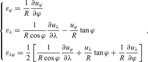
2.1 Differential relation between displacement and strain

The strain tensor on the earth's surface can be expressed in terms of displacements in spherical coordinates as (Melchier 1978; Savage et al. 2001)

1

where ϕ signifies the latitude, λ denotes the longitude and R stands for the average radius of curvature. In eq. (1), u_ϕ and u_λ represent the displacement of a point in latitude and longitude directions, and ɛ_ϕ, ɛ_λ and ɛ_λϕ represent three independent components of the strain tensor.

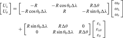
2.2 Segment approach to compute strain

The segment approach divides a study area into several units (e.g. triangulations) and computes the strain parameters for each segment. Finally, all individual results are integrated. The corresponding result is valid for a block. For example, the formula used by Savage et al. (2001) shown below is a specific equation [obtained through eq. (1) based on a Taylor series].

2

Therein, U_λ and U_θ represent displacement components, ω_ϕ, ω_θ and ω_γ are Euler vectors of the segment, R and θ₀, respectively signify the average radius of curvature and co-latitude of the segment centre, ɛ_λ, ɛ_λθ and ɛ_θ are the three components of strain tensor, θ and λ, respectively stand for the co-latitude and longitude, and Δθ and Δλ are the respective coordinate differences between the computing point and the segment centre.

2.3 Gridded approach to compute strain

The gridded approach normally establishes a functional relation between position and displacement with specific basis functions. It then computes the strain field by taking partial derivatives of the strain components in eq. (1) with respect to longitude and latitude. Three concrete methods are introduced below.

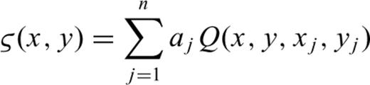
2.3.1 Multisurface function method

The multisurface function method was proposed by Hardy (1978). The principle is that any smooth mathematical surface can be approximated with any precision as a sum of regular mathematical surfaces, but a smooth mathematical surface cannot fit the data exactly because of errors in the data. In addition, the fitting accuracy is somehow affected by these errors. Liu et al. (2001) applied this method to computation of horizontal crustal movement in China using GPS data. The mathematical model used by Liu et al. (2001) is shown below.

3

Therein, ς (x, y) is the observed value, j represents the number of the adjustment node selected by fitting, n is the quantity of adjustment nodes, a_j are parameters to be determined, Q is a kernel, usually given in the form of Q(x, y, x_j, y_j) = ((x−x_j)²+ (y−y_j)²+σ²)^β, where σ is a smoothing factor (chosen according to the actuality), and β is an index parameter, usually set to 0.5, 1, 1.5 or –0.5. According to eq. (3), a_j can be computed easily. Their precision can be assessed using measurement adjustment theory.

The node information in eq. (3) is expressed in terms of plane coordinates. In terms of spherical distance, eq. (3) can be expanded further to

4

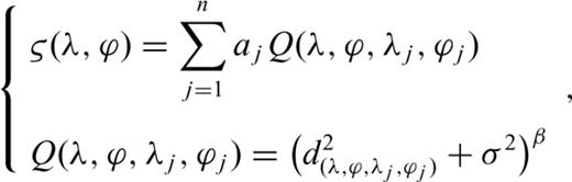
where is the spherical distance from node (λ, ϕ) to node (λ_j, ϕ_j). To calculate it easily, the unit of in this paper is set to 100 km.

2.3.2 Spherical harmonics method

Any function on a spherical surface is known to be expandable as spherical harmonics (Heiskanen & Moritz 1967). For example, a displacement (or rate) vector (U_e, U_n) can be expanded as

5

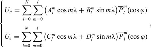
where N is the degree of truncation, stands for associated Legendre polynomials and A^m_l, B^m_l, C^m_l and D^m_l represent parameters to be determined. Based on the adjustment theory, we can solve those parameters and their errors in light of eq. (5). Then, the strain field can be computed using eq. (1). The precision of various strain parameters can be computed according to the covariance propagation law.

2.3.3 Least-squares collocation method

Least-squares collocation is explained in the literature, specifically in a report by Heiskanen & Moritz (1967). Least-squares collocation method is rigorous in theory, and it is useful for estimating non-random parameters [ in eq. (6)], the signal with random attributes [ in eq. (6)], and random errors [V in eq. (6)]. As described in this paper, we use this method to realize spatial interpolation and filtering based on a covariance function that describes the spatial correlations between any two points. In this process, we hypothesize here that the covariance function varies only with the distance between points. In the following, we first introduce the observation equation

6

where signifies the estimate of signals (including observed data and estimated data), G is the coefficient matrix of classical adjustment (if GPS velocity include rigid movement, ; else G= 0), denotes the parameters to be determined for the solution of classical adjustment (if the GPS velocity includes rigid movement, ; else ), L is the observed value, B_Z is the coefficient matrix for the signals in which identity matrix is for observed points but a zero matrix is for estimated points. Based on eq. (6), crustal movement can be described as whole movement depicted as , deformation depicted as and error depicted as V. Eq. (7) gives the final computing formula

7

where D_X stands for the covariance matrix of the signals at observed points, D_Z represents the covariance matrix of the signals at all nodes (including observed points and estimated points) and D_Δ is the covariance matrix of observed values.

Eq. (7) is a theoretical formula of the least-squares collocation. For computing large-scale crustal movement using eq. (7), it is necessary to determine the characteristics of the covariance distribution in advance. Detailed discussions can be found in reports by Jiang et al. (2003). Hereinafter, we adopt the following Gaussian covariance function.

8

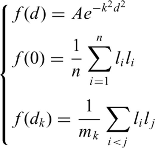
In that function, A and k represent the parameters to be obtained; l_i is the longitude velocity or latitude velocity from which the whole movement is deducted using the parameters in eq. (2). In addition, d_k is the distance between the observation points between i andj, and m_k is the count of point pairs at spherical distance d_k. Both A and k can be estimated using statistical approaches. The relation between covariance and distance d (in kilometres) can be constructed through linear fitting after logarithmic transformation (ln et al. (f(d)) = ln et al. (A) −k²d², where f(d) and d² are known, and we can solve A and k through linear fitting). Parameter d can be expressed as a function of the geodetic coordinate(λ, ϕ). Both D_Z and D_X in eq. (7) are constructed from f(d) in eq. (8), so that the strain field is calculable using the basic strain computing formula presented above. The corresponding error of the strain parameters can be determined from a posterior covariance matrix of the parameters and the covariance propagation law.

3 Example of Computing Simulation

3.1 Comparison of theoretical and computed results

We first assume a test area bounded by longitude 75°–135° and latitude 20°–50°. A velocity field (v_n, v_e) is therefore generated as a set of 1°× 1° grid data (mm a⁻¹), according to the following model.

9

Therein, the units of λ and ϕ are radians. Furthermore, rand () signifies a Gaussian random number of the error in the range of ±1 mm a⁻¹. Introduction of the random error is done to test the sensitivity of the computing methods to error because errors of various types affect real observations. We then compute the theoretical strain field and its spatial distribution using Eqs (1) and (9). At the same time, we can compute the parameters of maximum shear strain, surface strain and others.

Before presenting the computed results, the parameter selection method is briefly introduced. First, the triangular division method by Delaunay triangulation (Wessel & Smith 2006) is adopted for the segment approach. Any segment with an angle of less than 30° is removed. Then a set of strain parameters is computed as a unit for each triangulation before it is integrated into the final strain field. For multisurface methods, we should consider the following factors: the first is the current literature (Yang & Huang 1990; Huang & Liu 1992; Tao et al. 1992; Liu et al. 2001); the second one is the unit weight mean square error for fitting the multisurface function and the errors of the strain parameters; the last one is repeated trial calculations through comparison with theoretical results. Then the adjustment node is selected in the grid of 3.5°, with σ²= 1 and β= 1.5. Similarly, based on the unit weight mean square error for fitting spherical harmonics and the error of the strain parameters, and after repeated trial calculations with comparison to the theoretical result, the spherical expansion is made to a harmonic degree of 20. Finally, based on the least-squares collocation and signal covariance matrix introduced in eq. (8), parameters A= 57.5 and k= 0.00087 can be estimated as shown in Fig. 1 portraying theoretical maximum shear strain distributions in the simulating region for different computation methods. The input data with random errors are presented in Fig. 1(g) too.

Figure 1

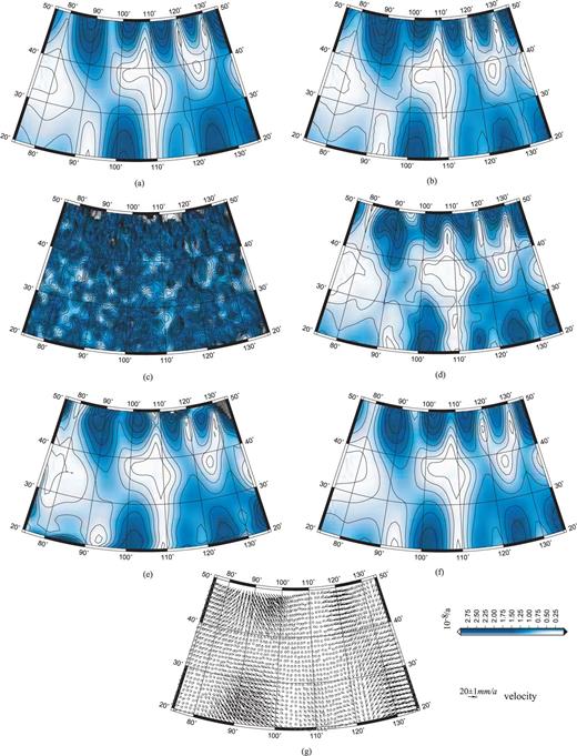
Maximum shear strain distributions in the simulating region obtained using different computation methods: (a) theoretical results, (b) results of Delaunay triangulation (not including random errors), (c) results of Delaunay triangulation (including random errors), (d) results of multisurface function (including random errors), (e) results of spherical harmonics (including random errors), (f) results of least-squares collocation (including random errors) and (g) input data (including random errors).

Open in new tabDownload slide

Comparison of these results in Figs 1(b)–(f) with the theoretical results presented in Fig. 1(a) reveals the following properties. The segment approach (Delaunay triangulation) gives an almost identical distribution if the input data do not include random error [Fig. 1(b)]. However, if a random error of ±1 mm a⁻¹ is included in the input data, then the results show a large discrepancy with the theoretical data [Fig. 1(c)]. This phenomenon results from the weak robustness of this method: only three points are used to compute the strain parameters (there are only 6 equations to solve 6 parameters, and the redundancy is 0), and all errors are included directly in the strain parameters. Furthermore, one point is often shared by two or more adjacent triangulations, in which case the deformation cannot be guaranteed continuity in adjoining triangulations. Furthermore, although the three gridded approaches show some difference in the contour distributions Figs 1(d)–(f), they fundamentally reflect the deformation features in the simulated region, that is, similar to the theoretical results. For the weak robustness of the segment approach, two methods were proposed to resolve the difficulty. One is interpolation and filtering of the displacement data before the computing strain. This method can improve the results, but it is impossible to reach the level of a theoretical estimate. A second method is to interpolate the input data before computing the strain field and then to filter the final results. However, some numerical tests show that this second method does not work well. The main reason is the impossibility of getting rid of observation errors by filtering.

3.2 Robustness of different strain computation methods

The previous discussions imply that different computing methods have different sensitivities to input data errors. Generally speaking, the segment approach is more sensitive than gridded approaches. The discussions presented above are based on white noise with standard error of ±1 mm a⁻¹. In the following, we further compare these methods for varying noise models.

We observe correlations between these methods through comparison of the consistency of the computed and theoretical results. The correlation coefficient is computed as

10

where x and y respectively represent two samples, and where n stands for the number of samples. The formula requires that the two samples be matched strictly (in this paper x_i and y_i are of the same node and express the same strain tensor).

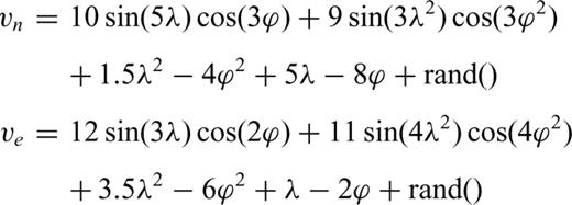
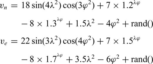
Eq. (9) is used to generate seven sets of simulation data with different random errors: 0.0 mm a⁻¹, ±0.5 mm a⁻¹, ±1.0 mm a⁻¹, ±1.5 mm a⁻¹, ±2.0 mm a⁻¹, ±2.5 mm a⁻¹ and ±3.0 mm a⁻¹. The area is bounded by longitude 75°–135° and latitude 20°–50°. Then we compute the corresponding strain parameters and correlation coefficients between the results obtained using the four methods and the theoretical strain result. The results depicted in Fig. 2 show that the correlation coefficient decreases as the random error (white noise) increases. The correlation for the Delaunay triangulation method decays quickly: it is reduced to 0.49–0.80 when the random error is ±1.0 mm. The correlation for the multisurface function method decreases to 0.90–0.98 when the random error is ±1.5 mm. The correlation for the spherical harmonics method becomes 0.90–0.98 when the error is ±2.5 mm, although the correlation for the least-squares collocation method decreases slowly as the random error increases, that is, the correlation coefficients decline to the range of 0.96–0.98 when the random error increases to ±3.0 mm. Specifically, if the input data include no random error, then all four methods produce similar results. If the error is 0–1.0 mm, then the three gridded approaches (methods) yield better results than the segment approach does. If the error is larger than 1.5 mm, then only the results of least-squares collocation method are more reliable than those of other methods. In addition, Fig. 3 shows that the latitude strain component has the weakest correlation, the shear strain component has a stronger correlation, and the longitude strain component has the strongest correlation. These phenomena coincide with the theoretical strain distribution, in which the signal-to-noise ratio in longitude is higher than that in latitude.

Figure 2

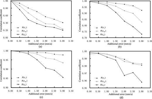
Correlation coefficients of results obtained using the four computing methods for different random errors: (a) Delaunay triangulation, (b) multisurface functions, (c) spherical harmonics and (d) least-squares collocation (standard errors of rand() are set, respectively, to 0.0 mm a⁻¹, ±0.5 mm a⁻¹, ±1.0 mm a⁻¹, ±1.5 mm a⁻¹, ±2.0 mm a⁻¹, ±2.5 mm a⁻¹ and ±3.0 mm a⁻¹).

Open in new tabDownload slide

Figure 3

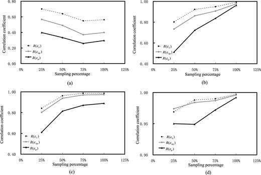
Correlation coefficients of the results for different resolution input data: (a) Delaunay triangulation, (b) multisurface functions, (c) spherical harmonics and (d) least-squares collocation (abscissa shows the sampling rate of input data for which rand() is set ±1.0 mm a⁻¹. 25 per cent is about in 2° grid input data, and 100 per cent are 1° grid input data).

Open in new tabDownload slide

3.3 Influence on strain rate computation caused by data sparseness

The distribution density of GPS points might affect the strain rate results: different methods have their own levels of sensitivity. To analyse this issue, we use correlation coefficients between calculation results with different input data sparseness generated by random function and theoretical results. The tested area is bounded by longitude 75°–135° and latitude 20°–50°; the error of input data is ±1.0 mm a⁻¹.

The results depicted in Fig. 3 shows that the Delaunay triangulation method cannot be compared to the other three methods. The correlation coefficient in 25 per cent input data is better than other rates when using the Delaunay method, which shows that the results are unstable and that the relative errors of small triangulation (high data density) are larger than those of big triangulation (low data density). The three gridded methods show the same characteristic, which illustrates that the correlation coefficient increases gradually along with the increase of the sampling rate of input data. Comparison of the three gridded methods indicates that the least-squares collocation method has the highest stability: the correlation coefficient is higher than 0.95 even with a sampling rate of input data of 25 per cent. In identical conditions, the correlation coefficient of the multisurface function method is 0.50–0.80; the value of spherical harmonics method is 0.60–0.85. Therefore, the influence of the input data resolution on the least-squares collocation method is less than that obtained using other methods.

3.4 Analysis of the computation of partly limited data

In practice, the spatial distribution of GPS points is not as homogenous as described above; it shows the absence of observation points in a large area. To verify the four methods, we consider limited input data. The data used in analyses are generated based on eq. (7). Moreover, the area is bounded by longitude 75°–135° and latitude 20°–50°. The first step is decimating 50 per cent of the data by resampling in the study region (Press et al. 2002) and then deleting data at two 10°×5° regions: one is defined as a region within (89°, 40°), (99°, 40°), (99°, 45°) and (89°, 45°); the other is (109°, 36°), (119°, 36°), (119°,,41°) and (109°, 41°), whose distribution is portrayed in Fig. 4(e). The remaining area retains the same data as those described in the section above. Then we compute the strain field using the four methods with the same parameters as those provided in the section above. Results (the maximum shear strain) are presented in Fig. 4.

Figure 4

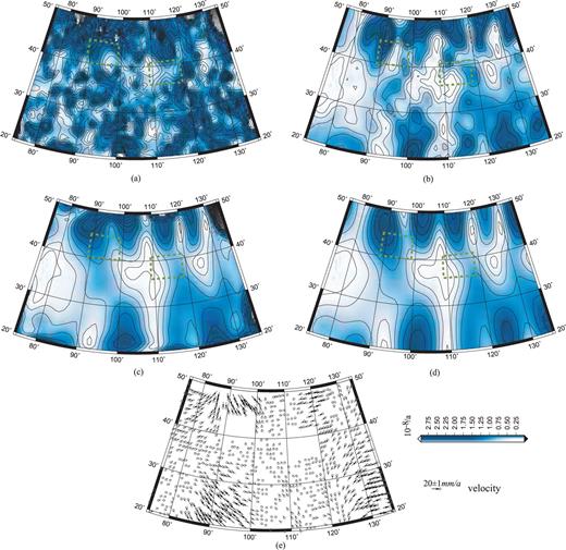
Results of the maximum shear strain rate field obtained using the four approaches (decimated 50 per cent limited data and deleted data in two regions which enclosed by the green dotted frame): (a) Delaunay triangulation, (b) multisurface functions, (c) spherical harmonic, (d) least-squares collocations and (e) input data (decimated 50 per cent limited data and deleted data in two regions).

Open in new tabDownload slide

Comparing the results portrayed in Fig. 4 and the theoretical values in Fig. 1(a) reveals that the result of Delaunay triangulation is the worst: the distribution and value of the strain rate contour differ from theoretical results. Three gridded approaches demonstrate good agreement, except for the edges and some details. In addition, the deleted data in two regions enclosed by the green dotted frame in Fig. 4 have little influence on the distribution of the strain rate. Generally, the least-squares collocation method yields the best result.

Figure 11

Results of the strain rate field in the λ direction and their error distribution during 1999–2004 (decimated 50 per cent data): (a) results for multisurface functions, (b) errors for multisurface functions, (c) results for spherical harmonic, (d) errors for spherical harmonic, (e) results for least-squares collocations and (f) errors for least-squares collocations.

Open in new tabDownload slide

3.5 Comparison of theoretical results and computation results on a medium scale

The analysis presented above has evaluated the reliability of different strain rate computation methods in a large scale. To elucidate the universality of these four methods, we analyse the application of these methods on a medium scale. When the study area is as large as the area of the Chinese mainland, we often devote more attention to the smooth change of the strain rate field. When the study area is medium-sized, we often devote more attention to the strong change. Furthermore, because the density of real GPS points is not uniform, it is difficult to estimate the strong change of the strain rate field on a large scale. The tested area is bounded by longitude 90°E–120°E and latitude 25°N–40°N. A velocity field (v_n, v_e) is therefore generated as a set of 0.5°× 0.5° grid data (mm a⁻¹), according to the following model.

11

Therein, the units of λ and ϕ are radians. Furthermore, rand () signifies a Gaussian random number of the error in the range of ±2 mm a⁻¹, which is two times that of the large scale example; the purpose is to study the robustness of different methods comprehensively. According to the rules of parameter selection explained above, the adjustment node is selected in the grid of 3.0°, with σ²= 1 andβ= 1.5 in the multisurface function method; the spherical expansion is made to a harmonic degree of 20 in spherical harmonics methods; the parameters A= 44.6 and k= 0.00175 can be estimated using the least-squares collocation method.

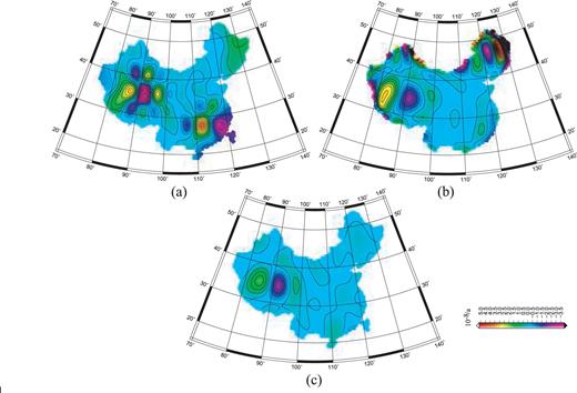
The Delaunay triangulation method is inferior to the other three methods gridded in both the distribution of contour and the strain rate value; Fig. 5 portrays the surface strain rate distributions in the simulated region for the three gridded methods. Presenting these results in Figs 5(b)–(d) for comparison with the theoretical results in Fig. 5(a) reveals that these three methods can all yield good results. In view of the edge effect, the multisurface function method is inferior to the spherical harmonics method. In turn, the spherical harmonics method is inferior to least-squares collocation.

Figure 5

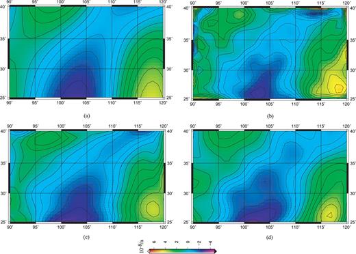
Results of the surface strain rate field using the three gridded approaches in medium scale: (a) theoretical results, (b) multisurface functions, (c) spherical harmonic and (d) least-squares collocations.

Open in new tabDownload slide

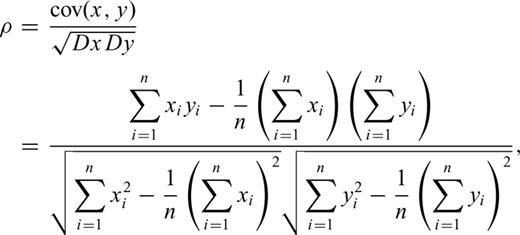
Based on the formula in eq. (11), Fig. 6 depicts the correlation coefficients between theoretical results and those obtained using four methods with different errors of input data. The distribution of correlation coefficients in Fig. 6 resembles that of Fig. 2 in some respects. The correlation coefficients of the Delaunay triangulation attenuate faster than those of the other three gridded methods. However, the correlation coefficients of the three gridded methods in Fig. 6 attenuate more slowly than in Fig. 2, which shows that the multisurface function and spherical harmonics methods are inferior to least-squares collocation method to some small degree. These characteristics show that the three gridded methods display little difference in intensive data distribution: each can yield a good result.

Figure 6

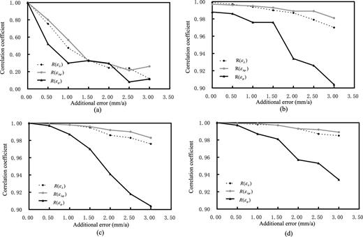
Correlation coefficients of the results obtained using the four computing methods in medium scale for different random errors: (a) Delaunay triangulation, (b) multisurface functions, (c) spherical harmonics and (d) least-squares collocation (standard errors of rand() are set, respectively, as 0.0 mm a⁻¹, ±0.5 mm a⁻¹, ±1.0 mm a⁻¹, ±1.5 mm a⁻¹, ±2.0 mm a⁻¹, ±2.5 mm a⁻¹ and ±3.0 mm a⁻¹).

Open in new tabDownload slide

We use the correlation coefficient between calculation results in different input data sparseness and theoretical result to analyse this issue. The error of input data is ±2.0 mm a⁻¹. The fundamental data are generated using eq. 10 in 0.5°× 0.5° grid. Results are depicted in Fig. 7. Results show that the correlation coefficient of the Delaunay triangulation method has random features in a low value, which illustrates that this method is not sensitive to the density of the input data in the range 1°–0.5°. The correlation coefficients of three gridded methods decrease gradually with the increase of a sparse level of input data. Results show that multisurface methods are inferior to spherical harmonics methods to a lesser degree, and that the spherical harmonics method is inferior to least-squares collocation to a lesser degree.

Figure 7

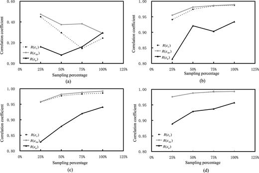
Correlation coefficients of the results for different resolution input data on a medium scale: (a) Delaunay triangulation, (b) multisurface functions, (c) spherical harmonics and (d) least-squares collocation (abscissa is the sampling rate of input data for which rand() is set as ±2.0 mm a⁻¹. 25 per cent is about in 1° grid input data; 100 per cent is 0.5° grid input data).

Open in new tabDownload slide

4 Example of Real Computing

The previous section described that the three gridded methods have better robustness and that they are superior for computing a medium-scale or large-scale strain field. In this section, we apply these three methods to compute the strain field using GPS data observed using the China Crust Movement Observation Network during 1999–2004. The purpose is to discuss the robustness and edge effect characteristics of these methods in view of actual observed data.

4.1 Analysis of strain rate results obtained using all GPS velocity fields for the Chinese mainland

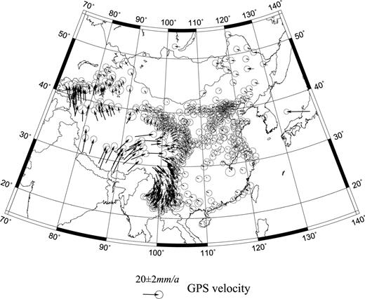
The GPS velocity fields using the GAMIT/GLOBK (Herring et al. 2006a,b) and QOCA (Dong et al. 1998) programs are used for this study. GAMIT is used to compute the single-day solutions of observation coordinates and satellite orbits, and QOCA is used to compute the global movement in the frame of ITRF2000. It is then converted into the velocity field relative to Chinese Mainland (Wang et al. 2003). The input data for strain rate computations are those of the regional velocity fields during 1999–2004 observed using the China Crust Movement Observation Network, which includes about 1000 points. The average error is ±1.6 mm a⁻¹ in the frame of Europe–Asia. Fig. 8 presents the distributions of the velocity fields obtained during 1999–2004. Reliability of the gridded method depends on how well the raw data are fitted. Table 1 presents fitting residuals of the velocity fields using the three gridded methods.

Figure 8

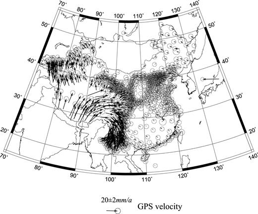
Distributions of GPS velocity fields from 1999–2004.

Open in new tabDownload slide

Table 1

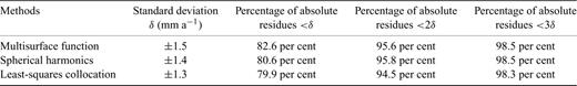
Fitting residuals of the velocity fields using the three gridded methods.

Open in new tabDownload slide

Table 1 shows that the post-fit residuals appear to form a normal distribution. Therefore, the distribution of the residues and their standard deviations imply that the fitted results obtained using these three gridded methods can reflect the most information of the velocity field and that the results are therefore applicable in strain rate field computations. Fig. 9 presents strain rate results in the λ direction and their error distribution. According to the rules of parameter selection presented above, the adjustment node is selected in the grid of 4.0°, with σ²= 1 and β= 1.5 in the multisurface function method. The spherical expansion is made to a harmonic degree of 20 in the spherical harmonics method. Parameters A= 20.5 and k= 0.00166 can be estimated using the least-squares collocation method.

Figure 9

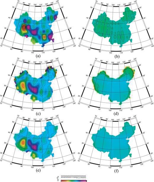
Results of the strain rate field in the λ direction and their error distribution during 1999–2004: (a) results for multisurface functions, (b) errors for multisurface functions, (c) results for spherical harmonic, (d) errors for spherical harmonic, (e) results for least-squares collocations and (f) errors for least-squares collocations.

Open in new tabDownload slide

As shown in Fig. 9, the results of spherical harmonics and least-squares collocation methods are consistent in the interior of the region. The edge effect of spherical harmonics is greater, especially in northeastern China, which implies that this method is affected by the geometric distribution of input data. The results of the multisurface function are consistent with those of the other two methods in western China, but the strain rate results show diversity in eastern China, which is inconsistent with the GPS velocity fields. The salient implication is that the multisurface function is also affected by the geometry distribution of input data. In view of the error distribution, the spherical harmonics shows an apparent edge effect that is stronger than those of the other two methods. Ignoring the edge effect, the errors of multisurface are greatest, and the errors of spherical harmonics and least-squares collocation methods are equal. Consequently, the edge effect and errors of least-squares collocation are smaller than those of other methods, reflecting the deformation information of GPS velocity fields, which is consistent with the results obtained from the simulation test.

4.2 Analysis of strain rate results obtained using decimated 50 per cent GPS velocity by sampling for the Chinese mainland

As presented in Fig. 8, there are about 1000 stations in GPS velocity vectors for the study region for 1999–2004. We will analyse the influence on the strain rate computation resulting from data sparseness. We use decimated 50 per cent data by sampling in Fig. 8 as input to calculate the strain rate parameters and their errors and to conduct a comparative analysis using the former results. Fig. 10 presents the decimated data; the parameter selections are the same as those presented in Fig. 9. Table 2 presents fitting residuals of the velocity fields using the three gridded methods in decimated data.

Figure 10

Distributions of GPS velocity fields during 1999–2004 (decimated 50 per cent data).

Open in new tabDownload slide

Table 2

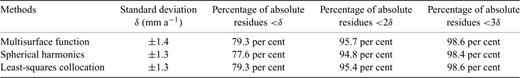
Fitting residuals of the velocity fields using three gridded methods (decimated et al. per cent data).

Open in new tabDownload slide

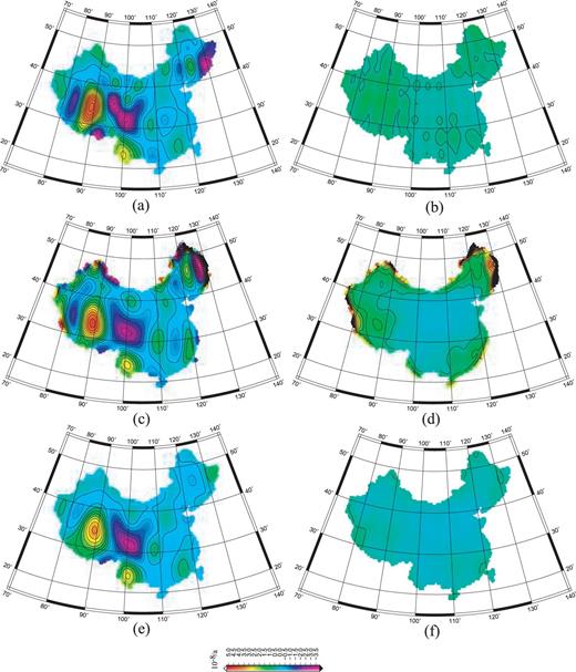
The residual distribution characteristic shown in Table 2 is the same as that of Table 1, which shows good normal distributions. No difference is discernible in view of the residual distribution from these two tables. Fig. 11 presents strain rate results in theλdirection and their error distribution in decimated data.

Comparison of Fig. 11 to Fig. 9 reveals that the results of multisurface function have changes that include squeezing increases in western China, and that the deformation scale decreases in southeastern China; errors are high too. The edge effect of spherical harmonics is more readily apparent; the scale is greater and extends to the inner Chinese mainland. The strain rate distribution and error distribution calculated from least-squares collocation is the same as the results shown in Fig. 9. These characteristics show that the edge effect of spherical harmonics is influenced by the distribution of input data. The edge effect is notable when the input data are sparse. The distributions of strain rate and errors calculated from multisurface function are also influenced by the distribution of input data. This method is not stable. The least-squares collocation method is affected by the distribution of input data to a lesser degree, and decimated data can meet the requirements of obtaining low frequency strain rate fields. Similarly, the same result can be obtained in the case of using latitude component of strain rate result.

To illustrate the difference between Fig. 9 and Fig. 11 quantitatively, the minus strain rate fields in the λ direction among all input data and decimated 50 per cent data are presented in Fig. 12. The primary characteristics are the same as described in the analysis presented above, including the fact that the differences are significant in western China and southeastern China when using multisurface function, and the edge effects are greater when using spherical harmonics. Otherwise, the minus results of these three methods all show differences in southwestern China, which displays tension in the west but pressure in the east. This characteristic accords with the background deformation of this region based on Fig. 9 or Fig. 11, which shows that some valid deformation information has been lost because of the use of decimated input data. However, the significant difference in southwestern China illustrates that the strain rate results in sparse regions of points that are easily affected by decimated input data.

Figure 12

Minus strain rate field in the λ direction among all input data and decimated 50 per cent data (Fig. 9–Fig. 11) (a) results for multisurface functions, (b) results for spherical harmonic and (c) results for least-squares collocations.

Open in new tabDownload slide

5 Discussion and Conclusions

The strain rate computation methods introduced in this paper are formulas for a sphere surface. Different methods have their respective advantages.

• (A)

  The segment approach (Delaunay triangulation method) is applicable for small area strain with few observation points. This method presents great disadvantages of weak robustness (no redundancy) and inability to satisfy the continuity of deformation caused by surveying errors. Therefore, to apply this method, two pre-treatments are useful for the segment approach. Numerical tests show that the interpolation and filtering in the displacement work better than those in strain work because observation errors are included in the strain computation for a triangulation; they cannot be filtered out. However, even if interpolation and filtering work, the results are no better than those obtained using spherical harmonics and least-squares collocation methods for computing the strain of a large area.

  We mainly discuss the strain rate calculation methods in a large scale and the simulated strain rate results are smooth. Therefore, gridded methods are superior to segment methods. To make strain rate results comparable among different regions, we use uniform parameters in light of one study area (for multisurface method, the parameters σ and β are uniform; for spherical harmonics, N is uniform; for least-squares collocation, A and k are uniform). In fact, these parameters should be a function of space, but it is very difficult to form this function under current distribution of GPS points. Consequently, the strain rate result calculated from these gridded methods might be a smooth approximation of the real distribution. However, if the real strain rate field contains some abrupt changes or if the study region is small, then the segment method might describe the deformation better than other gridded methods do. Furthermore, to describe the real deformation using the segment method, we should be sure of certain redundancies when solving strain parameters.

• (B)

  Based on tests of simulated data and real data, the fitting effect of multisurface function method is affected by some factors on which the choice of adjustment nodes and the parameter β have comparatively large influence, and on which parameter σ has a comparatively small influence. When choosing adjustment nodes, we should consider the quality of input data, the uniformity of the distribution of adjustment nodes and the covering scale of adjustment nodes. If the input data include minor errors, then the distribution of adjustment nodes should be dense. Otherwise, the distribution of adjustment nodes should be sparse. Furthermore, to evaluate the fitting effect, we should consider the unit weight mean square error and the strain parameter error, as well as the difference between the result of repeated trial calculations and the results of other methods.

  The selection of the degree of truncation is of great importance when using spherical harmonic method because this degree is related to the fitting effect and the precision of strain rate parameters. With the increment of degrees, the distribution of the strain rate field will show a considerable change. When this change is not significant with the increment of degree of truncation, we can determine the degree (N). In this process, we should compare the results with those obtained using other methods.

• (C)

  The robustness of the four strain computing methods inferred from large-scale simulation test results, ordered from best to worst, are the following: least-squares collocation, spherical harmonics, multisurface function and Delaunay triangulation methods. Numerical simulation shows that all four methods yield similar results if the input data do not include error. If the error contained in the input data is 0–1.0 mm, then the three gridded approaches produce better results than the segment approach. If the error is greater than 1.0 mm, then the least-squares collocation method yields the best result. In view of the influence to strain rate computation caused by data sparseness, the least-squares collocation method is affected to the least degree, and the spherical harmonics and multisurface function methods are affected to a greater degree. Furthermore, the least-squares collocation method can produce a reasonable strain field if for a decimated 50 per cent data set. In practice, all observation data are presumed to have error, so it is best to choose a method for which robustness is high.

• (D)

  Comparison of strain rate computing methods on a medium scale shows that the three gridded methods can meet the practical requirements in the intensive distribution of input data. Meanwhile, the sensitivities to errors of these three methods present a slight difference. The least-squares collocation method is better than the other two methods to a slight degree. In view of the influence on the strain rate computation caused by data sparseness, the correlation between calculation results and theoretical results of multisurface function and spherical harmonics attenuate faster than that of least-squares collocation with the data sparseness decreasing, which demonstrates that these two methods require a higher density of the data distribution.

• (E)

  In view of analysis of strain rate results for the Chinese mainland during 1999–2004, the stability of least-squares collocation is highest. It can produce a reasonable strain field for the decimated 50 per cent data set without a significant increase of strain rate errors. The edge effect of spherical harmonics is influenced by the distribution of input data, and the edge effect is notable when the input data are sparse. The distributions of the strain rate and errors calculated from multisurface function are influenced by the distribution of input data too. This method is not stable. The spherical harmonics and multisurface function methods are affected by the geometry distribution of input data, such as distortion of results in eastern China. Therefore, the least-squares collocation method is best in terms of robustness, edge effect, error distribution and method stability. The most important reason is that the covariance function of least-squares collocation is calculated from statistical data and can therefore reflect the real distribution of GPS velocity fields, which differs from other methods that depend on repeated trial calculations such as the harmonic degree of spherical harmonics and kernel function, smoothing factor and adjustment node selection of multisurface function methods. The parameter selection of least-squares collocation method is unaffected by humans. For that reason, different researchers can obtain identical results to those obtained using this method if the input data meet the real requirements.

Acknowledgments

The GPS data were obtained from the Engineering Research Center of the China Crust Movement Observation Network. Special thanks are extended to Prof. Wenke Sun, Prof. Min Wang, Prof. Qinwen Xi and Reviewers for their helpful advice. This work was financially supported by the National Science Foundation of China (40974005) and the specific fund of seismic industry (201008007).

References