Velocity–depth ambiguity and the seismic structure of large igneous provinces: a case study from the Ontong Java Plateau

Summary

1 Introduction

Large igneous provinces (LIPs) are peculiar geological regions that were formed rapidly (typically within a few million years) by spatially extensive magmatism (on the order of 10⁶ km²), such as continental flood basalts (e.g. Deccan Trap), oceanic plateaus (e.g. Ontong Java Plateau) and volcanic passive margins (e.g. North Atlantic igneous province) (Coffin & Eldholm 1994). LIPs are also commonly characterized by thick (20–30 km) igneous crust. In the framework of plate tectonics, these magmatic provinces are rather anomalous. Whereas large-scale mantle circulation associated with plate tectonics readily explains mid-ocean ridge magmatism and arc magmatism, the formation of LIPs is beyond these ‘normal’ modes of terrestrial magmatism. Because of their vast spatial dimensions, understanding why such magmatism takes place could potentially provide first-order constraints on mantle dynamics, such as the instability of the core–mantle boundary region (e.g. Richards et al. 1989; Larson 1991; Hill et al. 1992) and the efficiency of convective mixing (e.g. Takahashi et al. 1998; Korenaga 2004), but the origins of many LIPs still remain enigmatic owning mainly to the paucity of unambiguous data.

There is no active LIP at present, and most of LIPs are more than a few tens of millions years old, so it is generally not safe to expect the present-day mantle lying directly beneath a particular LIP to retain clues for its formation. If a LIP is created by the melting of a mantle plume head, for example, the mantle column beneath the LIP should exhibit strong thermal anomalies but only for a limited duration (on the order of 10 Myr) because such anomalies would eventually diffuse out. Even after the decay of thermal signatures, a chemically depleted residual mantle could still exist in the shallow mantle, though it may be gradually eroded away by convective currents in the mantle. For these reasons, therefore, the crustal part of a LIP, that is, the end product of mantle melting, is often the only reliable source of information on the dynamics of its parental mantle. Geochemical studies on LIP crust provide a range of elemental and isotopic compositions, by which we can estimate formation ages, eruption environments, the degree of depletion or enrichment in the parental mantle and mantle potential temperature (hypothetical temperature of mantle adiabatically brought to the surface without melting) (e.g. Tarduno et al. 1991; Fram & Lesher 1993; Thirlwall et al. 1994; Neal et al. 1997; Saunders et al. 1998; Michael 1999; Thompson & Gibson 2000; Kerr et al. 2002). Mantle potential temperature is particularly important as one of key control parameters in mantle melting (see Section 2) but is also difficult to estimate with confidence. This is because we need to know the composition of primary mantle melt to estimate the potential temperature, but geochemical sampling is limited to surface lavas, which are usually more fractionated than the primary melt. Back-fractionation correction, though often applied to alleviate the situation, can be notoriously non-unique when the composition of the parental mantle deviates from a normal pyrolitic composition (e.g. Korenaga & Kelemen 2000). It may also be unsettling to infer the entire crustal section solely from surface lava compositions when the crust is a few times thicker than normal oceanic crust.

Conversely, geophysical surveys, in particular wide-angle seismic refraction surveys, can sample the entire crust and potentially yield robust constraints on the gross characteristics of LIP crust (e.g. Mutter & Zehnder 1988; White &McKenzie 1989; Holbrook & Kelemen 1993; Barton & White 1997; Holbrook et al. 2001; Sallares et al. 2005). Seismological models of LIP crust, however, always suffer from the existence of non-unique solutions, so it is important to quantify the degree of non-uniqueness if we wish to interpret the crustal structure in terms of its causative mantle processes. Though the intrinsic non-uniqueness of crustal structure is reasonably well appreciated in the seismological community, how to actually quantify such non-uniqueness is still in an immature stage, and this is the focus of this contribution. Neither geophysical nor geochemical approach can provide a complete picture of LIP formation by itself, and understanding the strengths and weaknesses of each discipline is vital when synthesizing different kinds of observations.

Note that LIPs are occasionally defined to include hotspot islands such as the Hawaiian-Emperor seamount chain (e.g. Coffin & Eldholm 1994), but the term LIPs here is used to refer exclusively to massive igneous provinces formed in a relatively short period and does not include those produced by more steady-state and smaller-scale processes. Some LIPs seem to have geographical connections to presently active hotspots, which led to a hypothesis that a starting plume head and its succeeding plume conduit result in the formation of, respectively, a LIP and its nearby hotspot island chain (e.g. Richards et al. 1989). Under such assumption, the origins of LIPs may be inferred by mantle signals currently observed beneath their associated hotspots. Even in this case, well-resolved crustal structure remains of critical importance. In recent years, the origins of hotspot islands have become controversial (e.g. Anderson 2000; DePaolo & Manga 2003; Foulger & Natland 2003; Sleep 2003; Campbell 2005; Foulger et al. 2005; McNutt 2006), partly because the interpretation of mantle signals is often equivocal. A better understanding of the crustal component can help to reduce such ambiguity, as the interpretation of the mantle structure must always be consistent with that of the crustal structure.

This paper is organized as follows. First, the theoretical connection between the crustal structure and the parental mantle process is described (Section 2), in order to clarify how accurately the crustal structure should be estimated to warrant meaningful interpretation. Second, modelling strategies to construct crustal models, including both forward and inverse approaches, are reviewed to identify critical issues that are directly relevant to model uncertainty (Section 3). Then, an example with wide-angle seismic data collected over the Ontong Java Plateau is given (Section 4), followed by the discussion of possible future directions (Section 5).

2 Crustal Structure of Lips and the Nature of their Parental Mantle

When the mantle ascends beneath mid-ocean ridges, it cools down by adiabatic decompression, but the mantle solidus decreases more rapidly with decreasing pressures, so the ascending mantle eventually becomes hotter with respect to the solidus and starts to melt (unless the mantle is originally too cold) (e.g. McKenzie & Bickle 1988; Langmuir et al. 1992). Oceanic crust is the product of this mantle melting. At present, the potential temperature (T_p) of the normal mantle is estimated to be ∼1350 °C (Herzberg et al. 2007), and normal mantle starts to melt extensively at a depth of ∼60 km (Takahashi & Kushiro 1983). In this case, the degree of melting averaged over the entire melting column is ∼10 per cent, so the melting of normal mantle should produce ∼6-km-thick oceanic crust, which is consistent with the thickness of normal oceanic crust (White et al. 1992). This is a standard scenario for mid-ocean-ridge magmatism, which may be perturbed in a number of different ways. If, for example, the mantle temperature is higher than normal, it would start to melt at a greater depth, resulting in a higher degree of melting, a greater volume of total melt produced and a thicker crust. By measuring the variations of crustal thickness, therefore, one may hope to map out corresponding variations in the potential temperature of the parental mantle. Unfortunately, changing the mantle temperature is not the only way to modify crustal thickness because active mantle upwelling or more fertile mantle composition can also result in a thicker crust even with a normal potential temperature (e.g. Langmuir et al. 1992). This is why measuring crustal velocity, in addition to crustal thickness, becomes important. Crustal velocity can serve as a proxy for crustal composition, and the combination of total melt volume inferred from crustal thickness and melt composition from crustal velocity can discriminate between different scenarios. The first attempt to predict both crustal thickness and velocity based on a mantle melting model was presented by White & McKenzie (1989), and this theoretical approach has been elaborated since then, by incorporating the effect of active mantle upwelling (Kelemen & Holbrook 1995), by updating the mantle melting model and the relation between melt composition and crustal velocity (Korenaga et al. 2002), and by adding the effect of wet mantle melting (Sallares et al. 2005).

Theoretical predictions for the relation between the thickness of igneous crust and its P-wave velocity are shown in Fig. 1. A dominant control parameter is the mantle potential temperature, and there are two more model parameters, the ratio of rising velocity over surface divergence, χ, and the thickness of pre-existing lithosphere, b. The standard case of χ= 1 and b = 0 corresponds to passive mantle upwelling beneath a mid-ocean ridge, which predicts the crustal thickness of ∼6 km and the P-wave velocity of ∼7.1 km s⁻¹ for the normal T_p of 1350 °C, and thicker crust with higher velocity for hotter mantle (e.g. 16-km-thick crust with the velocity of 7.3 km s⁻¹ for T_p of 1500 °C). A higher degree of melting makes the melt composition more olivine-rich, resulting in the positive correlation between crustal thickness and velocity. In the case of active mantle upwelling, in which the mantle rises faster than surface divergence (i.e. χ > 1), more mantle mass is fluxed through the melting zone for a given potential temperature, resulting in thicker crust with little change in crustal velocity. On the other hand, the pre-existing lithosphere (b > 0) suppresses the final depth of melting, resulting in thinner crust. The mean pressure of melting increases in this case, but the mean degree of melting decreases as well, and these two effects on crustal velocity tend to cancel each other. Thus, when an igneous crust is 15-km thick, for example, its P-wave velocity could easily vary from ∼7.0 km s⁻¹ to ∼7.4 km s⁻¹, if the possibilities of active mantle upwelling and pre-existing lithosphere are taken into account.

Figure 1

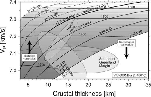
Theoretical predictions for the relation between crustal thickness and the P-wave velocity of the bulk crust, based on the method of Korenaga et al. (2002). Horizontal contours are for mantle potential temperature in °C, which is also shown in gray shading. Other contours correspond to different combinations of active mantle upwelling (χ) and the thickness of pre-existing lithosphere (b). Thick curve represents the standard case of passive upwelling beneath a mid-ocean ridge (χ= 1 and b = 0). Crustal velocities are values expected at the pressure of 600 MPa and the temperature of 400 °C. Also shown are the extents of existing thickness-velocity data from three LIPs: southeast Greenland margin (Korenaga et al. 2000), Galapagos volcanic province (Sallares et al. 2003; Sallares et al. 2005), and the Hatton Bank (White & Smith 2009). These observed velocities are the average velocity of the lower crust. To correct them for the bulk crustal velocity, they should be shifted downward by considering the cumulate nature of the lower crust (as indicated by ‘fractionation correction’), but also upward when crust is not very thick by considering residual porosity due to hydrothermal alternation (‘alteration correction'). See the main text for details.

Open in new tabDownload slide

One important assumption made in Fig. 1 is that the composition of the source mantle is normal (i.e. pyrolitic), so the effect of fertile (or depleted) mantle is excluded. A majority of existing mantle melting experiments were designed to understand the melting of a pyrolitic mantle, and as a result, it is still difficult to confidently predict the effect of different source compositions on mantle melting. Also, there are a number of different ways to perturb the mantle composition locally (e.g. Hirschmann & Stolper 1996), so invoking a non-standard source mantle could easily become an ad hoc exercise. A sensible strategy would therefore be to call for the possibility of compositional heterogeneity only when data cannot be explained by predictions with a normal pyrolitic composition.

The theoretical prediction of crustal velocity, as shown in Fig. 1, is based on the equilibrium crystallization of primary mantle melt, and there exist at least two processes that prevent the direct use of the diagram to interpret actual crustal structure. First, an igneous crust is usually believed to be internally differentiated as a consequence of melt migration through a steep geotherm near the surface; ophiolite and deep-sea drilling studies suggest that the lower crust is made mostly of crystal cumulates whereas the upper crust corresponds to fractionated liquids (e.g. Hopson et al. 1981; Kelemen et al. 1997; Wilson et al. 2006). The seismic velocity of the upper crust does not provide good constraints on chemical composition because it is known to be controlled mostly by porosity (e.g. Christensen & Smewing 1981; Detrick et al. 1994), leaving the lower crust as the sole source of compositional information. The seismic velocity of crystal cumulates is always higher than that of the solidified primitive melt (or the bulk crustal velocity), by ∼0.1–0.2 km s⁻¹ (Korenaga et al. 2002), so the lower-crustal velocity must be used as the upper bound on the bulk crustal velocity. If the average velocity of the lower crust is 7.2 km s⁻¹, for example, the bulk crustal velocity may be as low as 7.0 km s⁻¹ but cannot be higher than 7.2 km s⁻¹. The second complication comes from the possibility that even the lower-crustal velocity may be affected by porosity (due to hydrothermal alternation) if the crust is not very thick (Korenaga et al. 2002). As shown in Fig. 1, the passive upwelling of the normal mantle (with T_p of 1350 °C) is predicted to produce a 6-km-thick crust with the velocity of ∼7.1 km s⁻¹, but the lower-crustal velocity of the normal oceanic crust, which is expected to be higher than this value due to fractionation processes, is actually lower, being only ∼6.9 km s⁻¹ (White et al. 1992). The study of thermal cracking of oceanic lithosphere suggest that the effect of residual porosity decreases with increasing depth (Korenaga 2007). Thus, an observed lower-crustal velocity is likely to serve as the upper bound on the bulk crustal velocity when interpreting a thick LIP crust (>15 km), though this issue needs to be better quantified in future.

For LIPs, the number of well-resolved crustal models is limited, and three examples are given in Fig. 1: the southeast Greenland margin (Korenaga et al. 2000), the Galapagos volcanic province (Sallares et al. 2003; Sallares et al. 2005), and the Hatton Bank (White & Smith 2009), all of which employ joint refraction and reflection tomography with Monte Carlo uncertainty analysis as implemented by Korenaga et al. (2000). These velocities are lower-crustal velocities whereas crustal thicknesses are for the entire crust. The interpretation of these seismic observations is not straightforward as explained above, but some robust conclusions can still be made based on the sense of thickness–velocity correlation. A strongly negative correlation observed for the Galapagos volcanic province, for example, cannot be explained by the effect of residual porosity due to alteration, because this effect should be weaker for thicker crust. The negative correlation, if taken literally, indicates more active upwelling of colder-than-normal mantle, but such a scenario does not seem to be dynamically feasible, and this is the basis of the wet source mantle hypothesis for this LIP (Sallares et al. 2005). In contrast, the significance of a positive correlation, such as observed for the Hatton Bank, is more vague. It appears that the Hatton Bank data can be explained well by the moderately active upwelling (χ∼2) of hot mantle (T_p ∼1500 °C) with subsequent cooling by ∼200 K, but high crustal velocity for thicker crust is merely the upper bound on the bulk crustal velocity, which could be close to normal (i.e. ∼7.1 km s⁻¹), and the velocity of thinner crust is likely to be influenced by residual porosity. Clearly, it is important to improve our understanding of crustal genesis so that we can confidently infer the bulk crustal velocity from the observed lower-crustal velocity, and at the same time, more field data need to be collected from various tectonic settings, to build an ‘empirical’ knowledge base to complement this theoretical approach.

Also, when building such a knowledge base, it is vital to fully quantify the uncertainty of crustal velocity models. As Fig. 1 indicates, a P-wave velocity difference of 0.1 km s⁻¹ corresponds to a potential temperature difference of ∼100 K, and the accurate determination of both crustal thickness and velocity is essential to evaluate the likelihood of active upwelling or mantle source heterogeneity. The velocity of the lower crust is most diagnostic of the crustal composition, but it is also the most difficult part to accurately constrain. In active-source seismology, the crustal structure is usually constrained by the traveltimes of refracted waves (Pg) and reflected waves bounced off the Moho discontinuity (PmP). Because the lower crust does not exhibit a notable velocity gradient, most of refracted waves pass only through the upper crust and hardly sample the lower crust. The structure of the lower crust is, therefore, mostly constrained by PmP traveltimes, which are sensitive to crustal velocity as well as the Moho depth. When the PmP ray coverage is not sufficiently dense, it can be difficult to determine velocity and depth at the same time, resulting in velocity–depth ambiguity, that is, we cannot discriminate between thick crust with high velocity and thin crust with low velocity. This non-uniqueness issue of reflection traveltimes is well known (Bickel 1990; Stork 1992; Bube et al. 1995), but a practical strategy to quantify the degree of velocity–depth ambiguity for seismic tomography was not available until the introduction of depth-kernel scaling by Korenaga et al. (2000) (cf.eq. 13). Because of the limitation of computational resources available then, however, depth-kernel scaling was not fully utilized in their uncertainty analysis. Subsequent tomographic studies of LIPs have adopted the uncertainty analysis of Korenaga et al. (2000) with little modification even in recent years (e.g. White & Smith 2009). However, the popularization of high-performance computing now allows us to conduct a more complete assessment of velocity–depth ambiguity. As mentioned in Section 1, the purpose of this paper is to introduce a more satisfactory uncertainty analysis that can thoroughly explore velocity–depth ambiguity, which is explained in the next section.

3 Traveltime Modelling and Its Uncertainty

Estimating a crustal structure from seismic traveltimes may be done either by a forward or inverse approach. In either approach, the goal is to find a set of velocity models that are consistent with observed traveltimes. Such velocity models are sought by trial and error in the forward approach and by a more automated way in the inverse approach. In principle, the same result could be achieved using either approach, but finding just one successful model is already quite time-consuming with forward methods, leaving inverse methods as the only viable option to explore the vast model space of crustal structure. For model estimation, one needs to calculate at least the following two vectors (e.g. Tarantola & Valette 1982): (1) the mean model vector, or the expectation of the model vector defined as

1

and (2) the model variance vector defined as

2

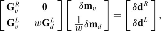
where m is a model vector, P(m) is its probability, and represents the model vector space. The probability P(m) is actually a conditional probability given the data vector d, that is, P(m) ≡ p (m|d), which can be further decomposed with the Bayes' rule as,

3

The probability p(m) is the prior, which contains a priori information on the model vector (e.g. p(m) = 0 if any velocity component is non-positive), the probability p(d) is called the evidence, serving as the normalization factor and the conditional probability p(d|m) is the likelihood of the observed data vector with regard to a given model vector and may be calculated as

4

where χ²(d, m) is the cost function that measures the misfit between data and model prediction, t_i and t^p_i are observed and predicted traveltimes, respectively, σ_i is one standard deviation of t_i, and N is the number of observed traveltimes.

The direct evaluation of the multidimensional integrals in eqs (1) and (2) is impossible in practice because the number of dimensions is usually on the order of 10³–10⁶ for crustal velocity models. Such direct evaluation would also be extremely inefficient because most of the model space does not contribute to the integrations; the likelihood decays rapidly to zero as the misfit between data and model prediction increases [eq. (4)]. A more tractable approach would be to approximate these integrals as (Matarese 1993)

5

and

6

where {m^f_i} is a set of successful models with similar data misfits (e.g. χ²/N ≈ 1) and M is the total number of such models. What these approximations make explicit is that there can be a number of equally valid models, and an obvious question is how to find all (or most) of them. To address this question, it is essential to understand how traveltime tomography works in some details.

In general, the relation between a successful model and observed traveltimes may be expressed symbolically as

7

where A is an operator that takes a velocity model m and calculates theoretical traveltimes between the source and receiver pairs implicit in d. Using a model vector m₀ that is close to m^f, the operator may be linearized using the first-order Taylor expansion as

8

and eq. (7) may be rearranged as

9

where the sensitivity kernel G, the model perturbation vector δ m and the traveltime residual vector δ d are defined as

10

11

and

12

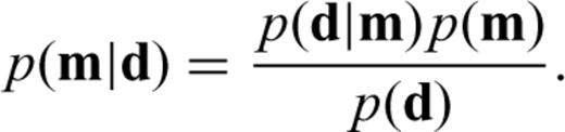
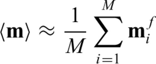
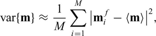
If the initial model m₀ is not close enough to m^f, the actual solution of eq. (9), δ m₀, does not bring us to m^f and we need to recalculate G and δ d using a new model vector, m₁=m₀+δ m₀, solve eq. (9) to obtain δ m₁, and repeat this process until δ d≈ 0. This is the essence of iterative linearized inversion used in seismic tomography. As the procedure described above depends critically on the choice of the initial model m₀, a straightforward strategy to collect a multiple number of m^f is to start with different initial models; Korenaga et al. (2000), for example, used randomly constructed 1-D initial velocity models to gather 100 successful models, from which they estimated a final model and its uncertainty on the basis of eqs (5) and (6).

For seismic tomography with reflection traveltimes (e.g. PmP), one further consideration is necessary. With depth kernel scaling, the linearized inverse eq. (9) takes the following form (Korenaga et al. 2000)

13

where the subscripts v and d, respectively, denote the velocity and depth components, the superscripts R and L are, respectively, for refraction and reflection traveltimes and w is the depth kernel weighting parameter. The actual inverse equation used in the tomographic method of Korenaga et al. (2000) is more involved because of damping and smoothing constraints (cf.Section 4), but the above simplified form is sufficient for discussion here. An essential point is that when the reflection ray coverage is not dense enough, the linear system of eq. (13) becomes singular, and the minimum-norm solution can depend strongly on the scaling parameter w. Smaller w, for example, leads to more velocity perturbations and less depth perturbations, even starting with the same initial model. If we wish to explore extensively the model space with velocity–depth ambiguity in mind, therefore, we need to not only use a variety of initial models but also test a range of the scaling parameter w for each of such initial models. Required computation was too time-consuming a decade ago, so it was implemented only partially by Korenaga et al. (2000); a number of initial models were used with w fixed to unity, whereas a range of w was tested only for one initial model. As parallel computing clusters have become commodities in recent years, such computational limitation is no longer an issue, as demonstrated in the next section.

4 An Example from the Ontong Java Plateau

In this section, wide-angle refraction data collected over the Ontong Java Plateau (OJP) (Miura et al. 2004) are used to create a worked example of the uncertainty analysis. Reasons to choose this particular data set include (1) that it is the largest oceanic plateau in the world (Coffin & Eldholm 1994), with several mysterious features that defy most of existing hypotheses for the LIP formation (Korenaga 2005) and (2) that the data of Miura et al. (2004) are so far the best published data for this plateau and yet have been analysed only with a forward modelling method. It is thus interesting, from scientific as well as technical points of view, to quantify how accurately existing seismic data may constrain the origin of this enigmatic plateau.

4.1 Data

The wide-angle refraction data reported by Miura et al. (2004) were acquired in 1995 with Japanese ocean-bottom seismometers (OBSs), using R/V Maurice Ewing's 20-gun tuned airgun array with a total chamber volume of 8510 cubic inch. As the details of the seismic survey are available in Miura et al. (2004), only essential points are given here. A 550-km-long seismic transect extends from the Indo-Australian Plate to the Pacific Plate, covering the Solomon Island Arc and the eastern edge of the Ontong Java Plateau (Fig. 2). Seventeen OBSs were deployed on the transect at an interval of ∼27 km, and the airgun array was fired at every 50 m (corresponding to a shot interval of ∼20 s). The transect is slightly bent in the middle, and I focus on the northern straight part with eight OBSs, which are labelled northwards from SAT11 to SAT18 (see the inset of Fig. 2).

Figure 2

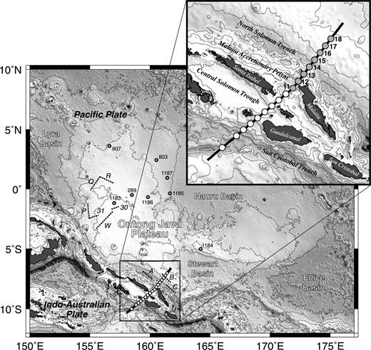
Bathymetry of the Ontong Java Plateau and the surrounding regions. Thick solid line denotes the seismic transect of Miura et al. (2004). Prominent geological features around the transect are labelled in the inset. Circles on the transect denote the locations of ocean bottom seismometers (see inset for the names of the instruments used in this study). Grey circles denote the locations of drilling sites, and dashed lines represent other previous seismic transects on the plateau: A–C (Furumoto et al. 1970), 31 and 32 (Murauchi et al. 1973), and P, Q, R and W (Furumoto et al. 1976).

Open in new tabDownload slide

The raw OBS data were reprocessed as follows. After removing exceedingly noisy traces (most likely due to instrumental glitches), traces were stacked with a bin width of ±100 m to reduce previous shot noise. Trace intervals after this horizontal averaging are ∼130 m. A bandpass filter with corner frequencies of 3 and 15 Hz was then applied, followed by predictive deconvolution to suppress ringy source signatures. Examples of processed data are shown in Figs 3 and 4. Data quality is variable among instruments. Data from SAT13 and SAT14 are exceptionally noisy, yielding only a limited number of traveltime constraints. Other instruments are generally of good quality, but no deep reflection phases can be identified with confidence from SAT17 and SAT18; when crustal thickness is tens of kilometres, it is not always easy to see the PmP phase clearly with this short interval of airgun firing because of previous shot noise.

Figure 3

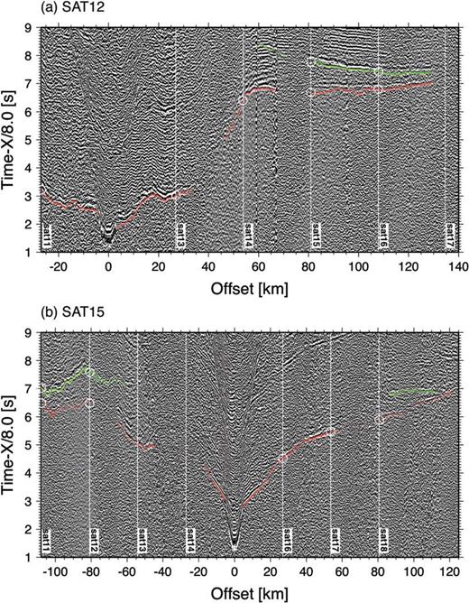
Processed seismogram for OBS (a) SAT12 and (b) SAT15, plotted with a reduction velocity of 8.0 km s⁻¹ and a range gain. Semi-transparent markings denote the picked traveltimes of Pg (red) and PmP (green). White vertical lines denote the locations of other instruments, and circles correspond to their traveltime picks at reciprocal relations (corrected for water-depth difference between instruments), demonstrating the consistency of phase identification among different instruments.

Open in new tabDownload slide

Figure 4

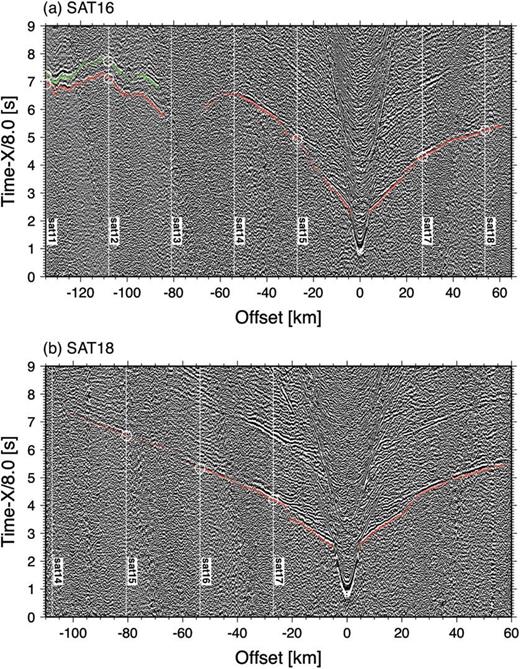
Same as Fig. 3 but for OBS (a) SAT16 and (b) SAT18.

Open in new tabDownload slide

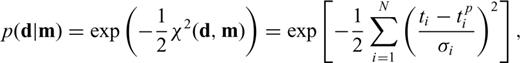
The traveltimes of the refraction (Pg) and reflection (PmP) phases were picked manually, and half a period of the first cycle of an arrival was used when assigning a picking error [σ_i in eq. (4)]. Picking errors vary from 50 ms to 150 ms, depending on the clarity of arrivals. In total, 4711 Pg and 1210 PmP traveltimes were collected (Fig. 5), and the source-to-receiver reciprocity was utilized to ascertain the internal consistency of phase identification among different instruments (Figs 3 and 4).

Figure 5

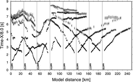
Picked traveltimes from all instruments are shown with their uncertainty as a function of model distance. Vertical lines denote OBS locations. Solid and open circles are for Pg and PmP, respectively, and data are shown at every five points for clarity.

Open in new tabDownload slide

4.2 Tomography results

A sheared velocity mesh is set up along the northern part of the seismic transect, with OBS SAT11 located at the southern end. The model domain is 249 km wide and 40 km deep from the seafloor, with a horizontal grid spacing of 1 km and a vertical grid spacing varying from 50 m at the seafloor to 1 km at the model bottom, amounting to ∼20 000 velocity nodes. The number of reflector nodes is 250 with a uniform 1-km spacing. A priori information on sedimentary layers is incorporated from Miura et al. (2004), and 200-m thick and 1.5-km thick sedimentary layers are hung from the seafloor for 0–85 km (the Malaita accretionary prism) and 85–249 km (OJP), respectively, with a top velocity of 2.0 km s⁻¹ and a bottom velocity of 3.0 km s⁻¹.

As the number of model unknowns greatly exceeds the number of data, a tomographic inversion needs to be regularized, and as in Korenaga et al. (2000), I employ both smoothing and damping constraints as follows

14

where L_Hv and L_Vv are horizontal and vertical smoothing matrices for velocity nodes, respectively, L_d is a smoothing matrix for depth nodes, D_v and D_d are damping matrices for velocity and depth nodes, respectively and the parameters λ_v, λ_d, α_v and α_d control the relative weights of these regularizing constraints with respect to data. Based on preliminary tests on model regularization, horizontal and vertical correlation lengths for velocity nodes are set to 10 km and 50 m, respectively, within the sedimentary layer, 5 km and 200 m at the top of the crust, 7 km and 2 km at the mid-crustal depth and 15 km and 5 km at the model bottom. The correlation lengths for the reflector nodes are sampled from the horizontal correlation lengths for nearby velocity nodes.

A large number of initial velocity models are prepared by hanging randomly-generated 1-D velocity profiles from the base of the sedimentary layer. A 1-D velocity profile is constructed from upper-crustal velocity v_U, mid-crustal velocity v_M, lower-crustal velocity v_L, upper-crustal thickness h_U and lower-crustal thickness h_L

15

where z is the depth measured from the base of the sedimentary layer, and v_U is randomly chosen from a range between 3 km s⁻¹ and 5 km s⁻¹, v_M between 5 km s⁻¹ and 7 km s⁻¹, v_L between 7 km ⁻¹ and 8 km s⁻¹, h_U between 3 km and 9 km and h_L between 15 km and 25 km. The reflector nodes are initially set at the same depth (i.e. a horizontal reflector), which is randomly chosen from a range between 25 km and 35 km. The depth kernel scaling parameter w is also randomized in a range between 10⁻² and 10².

The randomly generated initial models barely explain observed traveltimes, and their normalized χ² (i.e. χ²/N) usually exceeds 100; for comparison, χ²/N is less than unity when all of data misfits are within one standard deviation of observed data. When an initial model is located far away from successful models with small χ², damping is necessary to stabilize the iteration of linearized inversion. As in Korenaga et al. (2000), the damping weights α_v and α_d are determined not to exceed the upper limits on average velocity and depth perturbations, which are set to 3 per cent and 9 per cent per iteration, respectively. My strategy on the smoothing weights λ_v and λ_d is, however, different from that of Korenaga et al. (2000), who simply fixed these weights during iterations. When the data misfit is large as for the initial models used here, the smoothing weights need to be comparably large, but if I keep such large weights in the later phase of iterations, the effect of smoothing eventually dominates the inverse solution and the data misfit no longer improves. This may not be an issue when an initial χ² is not very large, but it also means that using constant smoothing weights could prevent us to freely explore the model space. Being able to arrive at a successful model (with χ²/N ∼1) starting from any initial model is of critical importance if we wish to quantify the model uncertainty (Section 3), so I introduce a misfit-dependent smoothing control as

16

where

17

For this study, I set as follows: a = 1, b = 50, λ_v,min= 30, λ_v,max= 400, λ_d,min= 3 and λ_d,max= 40, and using the misfit-dependent smoothing, most of initial models successfully led to models with χ² < 1 within ∼10 iterations. Finally, to take into account the effect of the data uncertainty on the model uncertainty, I also randomize observed traveltimes with the common receiver error of 50 ms and the traveltime error of 50 ms for each initial model, as in Korenaga et al. (2000).

Three examples of successful models are shown in Fig. 6. Models A and B (Figs 6a and b) were constructed from similar initial models (Fig. 6e), but a difference in depth kernel scaling (w = 42 for A and w = 0.04 for B) resulted in greater variations in the Moho depth for model A. Inversion with smaller w tries to seek a solution with smaller depth perturbations. Small w (0.11) similar to that of model B was used for model C (Fig. 6c), but its initial model has higher velocity and deeper Moho (Fig. 6e), and as a consequence, model C exhibits much greater velocity variations. Note that these models are equally valid in terms of data fit (Figs 6f and g), all having χ²/N ≈ 1. This diversity of successful models simply means that available traveltime constraints are too weak to determine the entire crustal structure reliably, but some parts of the crust still appear to be consistent among different models. The very purpose of doing the uncertainty analysis is to identify which part of the model we can rely on.

Figure 6

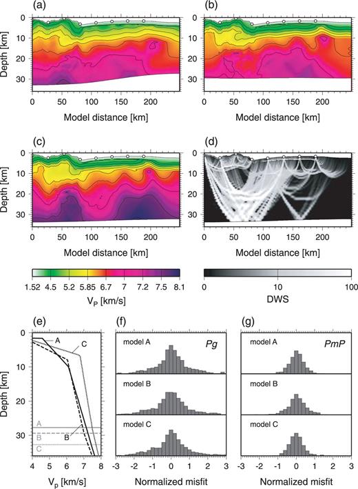
(a–c) Examples of successful crustal velocity models A–C. Values of the depth kernel scaling parameter w are (a) 42, (b) 0.04 and (c) 0.11. Colour shading represents P-wave velocity, and contours are drawn at every 0.5 km s⁻¹. (d) Derivative weight sum, which may be regarded as a proxy for ray density, for model C. (e) Initial 1-D velocity profiles and reflector depths. (f,g) Distribution of Pg and PmP traveltime residuals for models A–C, normalized by picking uncertainty.

Open in new tabDownload slide

The results of the Monte Carlo uncertainty analysis are summarized in Fig. 7. I collected 2000 models with χ²/N ≈ 1, and used the first 1000 models to calculate the mean (Fig. 7c) and the standard deviation (Fig. 7d). I repeated the same calculation with the other 1000 models, and differences in the mean and the standard deviation are shown in Figs 7(e) and (f), respectively. For most of the model domain, the difference in the model mean is less than 0.5 per cent, and that in the standard deviation is on the order of 0.01 km s⁻¹ for velocity nodes and ∼0.1 km for depth nodes. When a Monte Carlo approach is used, a key question is always how many trials are needed to achieve convergence. Using a large number of trials combined with cross validation, as attempted here, is one possible way to address such concern. Though this approach needs to be formulated more rigorously in future, the current results appear to be promising. The standard deviation of successful models indicates that the upper to middle crustal structure beneath the Malaita accretionary prism (30–80 km) and the middle to lower-crustal structure beneath OJP (90–140 km) are reasonably well resolved with 1 σ < ∼0.1 km s^-1 (Fig. 7d). In contrast, the lower-crustal structure beneath the accretionary prism is characterized with much higher standard deviations, which is interesting because this part also has the densest PmP coverage (Fig. 6d). This is a good example of non-linear model sensitivity; model uncertainty does not always correlate with linear sensitivity indicated by ray coverage (Zhang & Toksöz 1998).

Figure 7

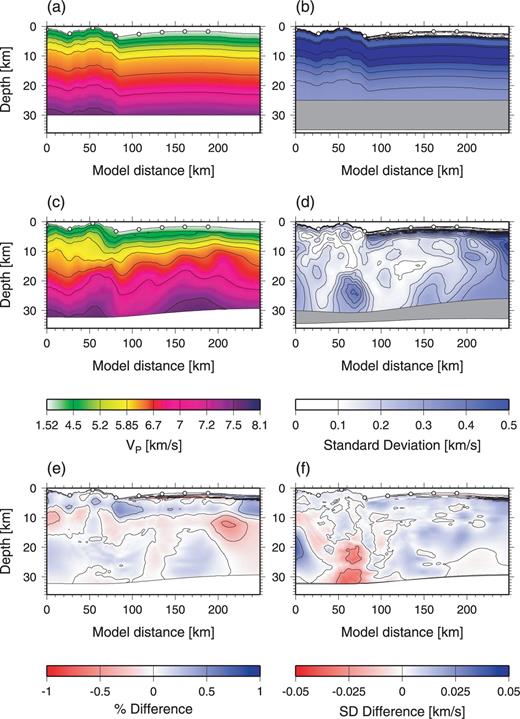
(a) The average of first 1000 initial models used in the Monte Carlo search. (b) The standard deviation of those initial models. Grey region denotes the range of initial reflector depths (30 ± 5 km). (c) The average of first 1000 successful models with χ²≈ 1. (d) The standard deviation of those models. Grey region denotes the mean Moho profile with one standard deviation. (e) Percentage difference between the model average from the first 1000 successful models and that from the second 1000 models. (f) Difference in standard deviation for those two model ensembles. Grey region denotes the mean Moho profile with the difference in standard deviation (mostly <0.1 km).

Open in new tabDownload slide

To illustrate the varying degree of velocity–depth ambiguity in the model, the correlation between crustal thickness and lower-crustal velocity among the ensemble of successful models is shown for two regions, one beneath the accretionary prism and the other beneath the plateau (Fig. 8a). The lower crust here is defined to occupy the lower two-thirds of the whole crust, and the average velocity of the lower crust is calculated for each model. The lower-crustal velocity beneath the accretionary prism is poorly constrained, exhibiting a strongly positive correlation with the crustal thickness, whereas that beneath the plateau is clustered around 7.15 km s⁻¹ despite relatively large variations in the crustal thickness. Using a range of depth kernel scaling is important to explore such velocity–depth ambiguity (Fig. 8b). For the case of the structure beneath the accretionary prism, for example, the uncertainty of the lower-crustal velocity would not be fully revealed even by an extensive Monte Carlo search if a conventional choice of w = 1 is adopted.

Figure 8

(a) Covariation of whole crustal thickness and lower-crustal velocity, both averaged over a subdomain between 40 and 90 km (grey circles) and that between 90 and 130 km (solid circles). The lower crust here is defined to be the lower 2/3 of the entire crust. Ellipses denote the 68 per cent confidence regions for these two distributions, and star represents the velocity model of Miura et al. (2004). (b) Average lower-crustal velocity for those two subdomains as a function of the depth kernel weighting parameter w.

Open in new tabDownload slide

Note that intracrustal reflection phases can be identified in some instruments (Fig. 4), but unlike the study of Miura et al. (2004), only the first arrivals (Pg), together with the reflection off the Moho (PmP), are considered in this study. These intracrustal reflection phases are too fragmentary to warrant the modelling of additional interfaces within the crust; each of such interfaces would lead to its own velocity–depth ambiguity. It has long been known that a smoothed velocity structure can be properly recovered from first arrivals only (e.g. Slichter 1932), and given the purpose of estimating the average lower-crustal velocity, it is deemed appropriate to limit ourselves to the class of smoothly varying velocity models.

4.3 Petrological implications

The useful portion of the crustal velocity model, that is, the lower crust with low enough standard deviations, is only a small fraction (90–140 km) of the entire model domain, and it may not be warranted to discuss the origin of this gigantic plateau based on the interpretation of such a small crustal volume. Nonetheless, this is the first time a well-defined crustal structure is found within OJP and its implications for the parental mantle deserve attention. As will be shown, it is difficult to explain the observed crustal structure in the framework of melting of normal pyrolitic mantle, and this study clearly points to the need for more extensive field data acquisition as well as multidisciplinary efforts for a better hypothesis for the genesis of OJP.

Based on the theoretical predictions for the relation between crustal thickness and the P-wave velocity of the bulk crust (Fig. 1), the crustal structure for 90–140 km, with an average lower-crustal velocity of 7.2 ± 0.1 km s⁻¹ and a whole crustal thickness of 30 ± 2 km, may be interpreted as a result of highly active upwelling (χ∼8) of a moderately hot mantle (T_p ∼1400 °C) beneath a mid-ocean ridge (Fig. 9a). Though the error ellipse (corresponding to the 68 per cent confidence region) is wide enough to allow less active upwelling (χ of only ∼2) of hotter mantle (T_p ∼1500 °C), two factors act against exploring the higher end of the velocity range. First, as explained in Section 2, the lower-crustal velocity serves as an upper bound on the bulk crustal velocity especially when the crust is as thick as 30 km. Secondly, the theoretical predictions for crustal velocity are made at a pressure of 600 MPa and a temperature of 400 °C. While there is no need to correct for pressure in this case, the temperature of the lower crust under consideration is likely to be ∼200–300 °C given the age of OJP (∼120 Ma), so a correction to the reference temperature of 400 °C would result in a decrease in velocity by 0.04–0.08 km s⁻¹ (Korenaga et al. 2002).

Figure 9

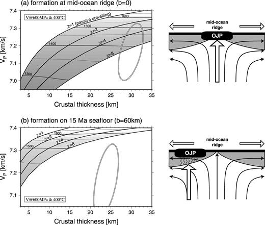
Interpretation of the crustal structure of OJP (from model distance 90–130 km) using the theoretical predictions based on the melting of a pyrolitic mantle (Fig. 1). As in Fig. 8(a), ellipses denote the 68 per cent confidence region of whole crustal thickness and lower-crustal velocity. (a) Case of OJP formation at a mid-ocean ridge (the thickness of pre-existing lithosphere b is zero). (b) Case of OJP formation on 15 Ma seafloor (b=60 km). In (b), the thickness of pre-existing oceanic crust (6 km) is subtracted from the observed crustal thickness. Both theoretical predictions are based on the method of Korenaga et al. (2002).

Open in new tabDownload slide

The crustal structure becomes even less comparable with theoretical predictions if we consider a more realistic eruption environment. The tectonic setting of the formation of OJP is not well resolved because OJP was formed during the Cretaceous Quiet Period when the geomagnetic field did not reverse, but the geology of the surrounding seafloor suggests that OJP may have formed on ∼15–30 Ma seafloor created by a super-fast spreading centre (Larson 1997). The thickness of pre-existing lithosphere in this case is ∼60–80 km (Korenaga 2005, Fig. 3a), so the theoretical predictions of crustal velocity and thickness for the case of b = 60 km is shown in Fig. 9(a). Here, the thickness of newly emplaced crust associated with the OJP formation is estimated to be 24 ± 2 km, assuming that the pre-existing oceanic crust has a normal thickness of 6 km. If we wish to explain the observed crustal structure with the melting of a pyrolitic mantle, we need to invoke extremely fast mantle upwelling (χ≫ 10) with a marginal thermal anomaly, which seems dynamically implausible.

A couple of alternative views are possible. The first option is simply to disregard this particular seismic constraint as the crustal volume may be too small to be representative of the entire plateau. Also, the seismic transect of Miura et al. (2004) does not sample the central part of OJP, and we may be looking at a locally anomalous part of the plateau. Gladczenko et al. (1997) proposed that the lower crustal velocity of OJP may be as low as 7.1 km s⁻¹ by reprocessing vintage seismic data from other parts of OJP, but given the quality of those data collected during 1960s and 1970s, it is probably not wise to take this coincidence at face value. Note that they also suggested that such crust can be interpreted as ponded and fractionated primary picritic melts later recrystallized as granulite facies assemblages, but, unfortunately, this interpretation is based on a misunderstanding of the work of Furlong & Fountain (1986). The second option is that the assumption of a pyrolitic source mantle is incorrect. The melting of a more fertile mantle may be able to explain the crustal structure with less drastic active upwelling; even with passive upwelling, for example, a mantle enriched with subducted oceanic crust can generate thick crust (∼15 km) with the bulk crustal velocity of ∼7.0 km s⁻¹ (see fig. 17 of Korenaga et al. 2002). As explained in Section 2, it is difficult to pinpoint the nature of a putative non-pyrolitic mantle. What can be said with certainty is that, by reductio ad absurdum, something other than a pyrolitic mantle is required. Because fertile mantle is usually chemically denser than the normal mantle, however, this notion of a fertile source mantle may also explain other enigmatic features of this plateau such as submarine eruptions and anomalous subsidence (Korenaga 2005). Fortunately, a much more extensive seismic survey was recently conducted on OJP (Miura et al. 2010), so these issues can be pursued further if a comprehensive tomographic analysis is applied to the new field data.

5 Discussion and Outlook

In studies of the origin of LIPs, crustal velocity structures are used to go beyond just crustal processes and constrain the dynamics of their parental mantle, based on the theory of mantle melting and crustal genesis. A simple genetic connection between the igneous crust and the parental mantle, characterized by single-stage mantle melting, allows us to investigate past mantle dynamics from present crustal structure, but using this connection properly is not a trivial task, involving petrology, geodynamics, seismology and rock physics. As crustal seismology is the only way to sample a thick LIP crust at all depths, however, it is important to keep improving this seismological approach. The unique nature of compositional information stored in the crustal velocity structure more than compensates for the complexity of the theoretical inference.

As explained in Section 2, major theoretical issues that remain to be explored include (1) the degree of internal chemical differentiation during the formation of igneous crust, (2) the effect of residual porosity on the lower-crustal velocity, primarily as a function of crustal thickness and (3) the effect of non-standard source composition on mantle melting. The first two are essential for estimating the seismic velocity of the hypothetical bulk crust from the observed lower-crustal velocity. It is also important to collect field data that are easy to interpret. In this regard, oceanic LIPs may be ideal because the evolution of oceanic lithosphere, on which those LIPs are formed, is much better understood than that of continental lithosphere so that accounting for the effects of pre-existing lithosphere is more straightforward. Volcanic passive margins, for example, mark a transition from continental to oceanic lithosphere, and this transitional nature has been a source of ambiguity in the interpretation of crustal structure and thus the underlying mantle dynamics (e.g. Korenaga et al. 2002; White & Smith 2009). Oceanic plateaus formed in the middle of ocean basins (e.g. OJP) do not suffer from such ambiguity. Most of those plateaus are yet to be investigated, offering rich opportunities for marine geophysics.

All of the issues associated with estimating a velocity model from field observations may be reduced to how accurately we can evaluate the high-dimensional integrals of eqs (1) and (2) or their approximations [eqs (5) and (6)]. Put it simply, what matters here is how to collect all of the representative solutions in an efficient way, and this is a problem known as ‘importance sampling’ in statistics. Markov chain Monte Carlo (MCMC) methods are commonly applied to such problem (e.g. Liu 2001; Sambridge & Mosegaard 2002), but their direct application to traveltime tomography is impractical because the number of model parameters is prohibitively large; for MCMC methods to be computationally tractable at present, the number of parameters needs to be on the order of 10–100. MCMC methods are still attractive, however, because they offer a formalism to test the convergence of sampling, and it may be possible to reduce the number of model parameters drastically by treating, for example, the parameters needed to construct initial models as effective model parameters. In the case of the example given in Section 4, there are only five parameters, v_U, v_M, v_L, h_U and h_L. We may also include other key parameters that govern the tomographic inversion, such as the depth kernel scaling parameter w, correlation lengths and smoothing weights, and the number of effective parameters is still on the order of 10. At present, correlation lengths and smoothing weights are determined largely by trial and error, and these parameters can potentially create some bias in the exploration of the model space. An MCMC approach with the notion of effective model parameters would thus make the entire inversion process not only more complete but also more objective.

Revisiting the active-source seismic data from OJP with traveltime tomography yielded a crustal velocity model with its uncertainty fully quantified and also provided solid field evidence that is clearly inconsistent with the melting of a pyrolitic mantle, motivating further thoughts on the origin of oceanic plateaus in general. As the true value of the crustal structure of LIPs lies in its petrological interpretation, building just one model that can explain data should not be the goal of seismic data analysis. Finding a multitude of successful models in a systematic manner is essential to quantify model uncertainty, without which model interpretation bears little significance.

Acknowledgments

The author thanks Dr. Kiyoshi Suyehiro for a permission to analyse the OBS data collected by his group and Dr. Seiichi Miura for assisting the transfer of the raw OBS data. Reviews by Editor Ingo Grevemeyer, Emilie Hooft and an anonymous reviewer were helpful to improve the clarity of the manuscript. Most figures were prepared with the GMT system (Wessel & Smith 1995).

References