


Summary
The measurement of SKS splitting parameters is widely used for the study of deformation in the upper mantle, but the misalignment of the station horizontal components, for example misorientation of the sensors, may result in false measurements. In this paper, we suggest that the splitting analysis should be repeated with different assumed angles of misalignment. Two criteria can be applied to correct the measurement of the SKS splitting parameters: (1) the horizontal rotating angle should produce the global minimum transverse energy, as determined using the least transverse energy method; (2) there should be consistent results between the least transverse energy method and the minimum eigenvalue method. Model tests show that the method is suitable for complex anisotropy models, such as two-layer anisotropy.
1 Introduction
Shear wave splitting is increasingly measured and used to describe the anisotropy of the Earth. Shear wave splitting measurements from the SKS phase are routinely used to study the finite strain caused by deformation in the upper mantle (Vinnik et al. 1989; Silver & Chan 1991; Savage 1999; Evans et al. 2006). Large-scale mantle anisotropy is caused by the strain-induced preferred orientation of minerals, mainly olivine. Splitting measurements characterizing the orientation of the strain fields indicate the geological structure of the mantle.
Core–mantle refracted shear waves (e.g. SKS and SKKS), travelling as P waves within the liquid core, arrive at stations almost vertically. These converted shear waves, propagating through the isotropic mantle on the receiver-side of their paths, are polarized linearly in the ray path plane, that is, their transverse component has zero amplitude. A shear wave passing through an anisotropic region along its ray path splits into two orthogonally polarized quasi-shear waves. If the symmetry axes of the anisotropic region have a fixed orientation over a significant portion of the upcoming ray path, the two splitting shear waves can arrive at the station with notably different times. The interference between the two waves results in the elliptical particle motion of the recorded shear phases. The two splitting parameters, the fast polarization direction (φ) and the splitting time between the fast and slow waves (δt), can be interpreted in terms of the preferred mineral orientation in the upper mantle.
Several methods are available to evaluate the optimal pair of splitting parameters Φ and δt. The most common methods are based on correlating the wave components (hereafter RC; e.g. Bowman & Ando 1987), minimizing the energy of the transverse component (hereafter SC; e.g. Silver & Chan 1991) or minimizing the eigenvalues of the covariance matrix (hereafter EV; e.g. Silver & Chan 1991). Modifications of existing methods also have been developed. For example, Wolfe & Silver (1998) retrieved splitting parameters for noisy signals by stacking misfit functions. Chevrot (2000) developed a method that estimates the splitting parameters from the relative amplitudes of the radial and transverse components as a function of the incoming polarization angle. Menke & Levin (2003) suggested fitting the observed waveforms with anisotropic models. Many studies have been done to ensure reliable measurements of the shear wave splitting parameters. For example, an appropriate bandpass filter and window length for the analysed signals are recommended by Vecsey et al. (2008). Methods have been developed to reveal the multiple layers of anisotropy at some stations (e.g. Silver & Savage 1994; Levin et al. 1999; Liu et al. 2001; Polet & Kanamori 2002).
When a seismic station is deployed in the field, especially a temporary one, misorientations of the sensor are inevitable. The causes of the misorientation vary, and may include the effect of the local magnetic field or installation mistakes. In this paper, we present a reliable technique for the splitting parameters measurement when misalignment of the horizontal components happens. This method is tested on synthetic data and applied to the permanent station ULN with promising results.
2 Measurement of SKS Splitting Parameters on Synthetic Waveforms with Misalignment of the Horizontal Components
We synthesize a damped sinusoidal signal with BAZ as the incident SKS phase. When the SKS passes through an anisotropic layer, the waveform would split into two orthogonally polarized quasi-shear waves with a fast direction of φ0, and the wave in slow direction is delayed by δt0 to represent a slow wave (another wave in the fast direction is a fast wave). We then summed the amplitudes of fast and slow waves and obtained a synthetic SKS phase on the N–S and E–W components or the radial and transverse components. Our first example is of a synthetic waveform with a backazimuth (BAZ) of 120° and dominant periods T = 8 s. The waveform splits with parameters φ0 = 50° and δt0= 2.0 s. Three measurement methods, SC, RC and EV, are used to calculate the splitting parameters (Fig. 1). The grid search with the SC, RC and EV methods was used with an increment of 1° for φ from 0 to 180°, and 0.02 s for δt from 0 s to 4 s.
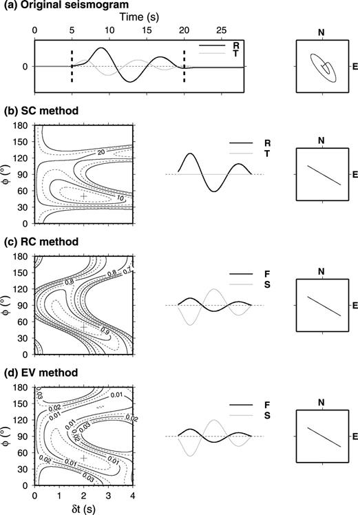
Splitting measurements for the synthetic waveform with a backazimuth of 120° and splitting parameters φ0= 50°, δt0= 2.0 s. (a) The synthetic original seismogram. The left panel shows the radial (bold line) and transverse (grey thin line) components and the time window (vertical dash line) of the SKS phase analysed. The right panel shows the initial particle motion. (b) The measurement of splitting parameters by the SC method. The left panel is the contour map of the energy on the transverse component with the best-fitting splitting parameters (φ= 50°, δt= 2.0 s) shown with the cross. The middle panel shows the corrected radial (bold line) and transverse (grey thin line) components, and the right panel is the corrected particle motion. (c) Same as (b) but by the RC method. The contour map shows the correlation coefficient. The bold line and the grey thin line in middle panel are the corrected fast and slow components, respectively. (d) Same as (c) but by the EV method. The contour map shows the minimum eigenvalue.
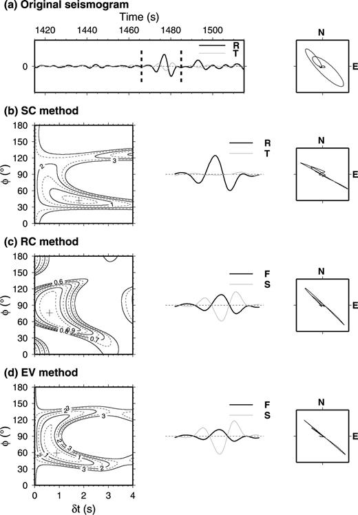
According to BAZ, the radial and transverse components are obtained from the east–west and north–south components recorded by a seismic station. However, the radial and transverse components will not be recovered correctly when east–west and/or north–south sensors are misoriented. We define θ as an angle between the true north and the orientation of the ‘north’ component of the sensor. θ is positive when the ‘north’ component is west of north, so that to correct it a clockwise rotation is needed. If we assume that the sensor is rotated towards east by a degree of 20°, we can synthesize a second example with the same parameters as the first example. Fig. 2 shows the measurement splitting parameters by the SC, RC and EV methods.
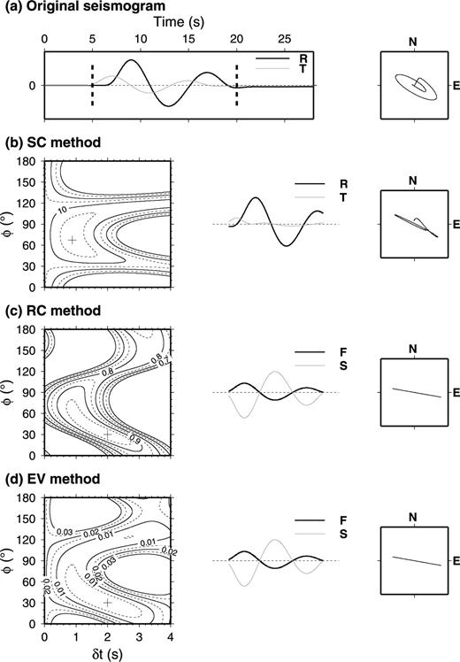
The same content as in Fig. 1, except that the north and east components were rotated clockwise by 20° to represent misalignment before the splitting measurements. After measurement, the best-fitting splitting parameters are φ= 67°, δt= 0.88 s by the SC method in (b), φ= 30°, δt= 2.0 s by the RC method in (c) and φ= 30°, δt= 2.0 s by the EV method in (d).
Although the correct splitting parameters were evaluated by the three methods with correct sensor orientation (Fig. 1), they could not be measured in the case where there is misorientation (Fig. 2). We repeat the measurement of the splitting parameters using different values of θ to revise the horizontal components and plot the measurement of φ varying with θ in Fig. 3. In Figs 3(a) and (b), it can be seen that the transverse energy reaches a global minimum, and that the three methods result in the correct splitting parameters (only φ is shown in Fig. 3) when θ = 0° and θ=−20° for the first and second examples, respectively.
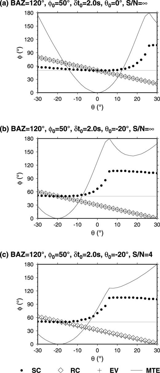
The fast direction (φ) variation with the correction angle θ (rotating the horizontal components clockwise). (a) The seismograms measured are same as those in Fig. 1(a). (b) The seismograms measured are same as those in Fig. 2(a). (c) The seismograms measured are same as those in Fig. 4(a). The results of the fast direction (φ) from three methods, SC (closed circles), RC (diamonds) and EV (crosses), become consistent when an appropriate correction angle θ is used. The minimum transverse energy (thin line) varying with θ is plotted in the same panel after normalization, and the transverse energy always reaches a global minimum at θ=θ0.
Thus, if we do not have accurate information about the misorientation of the seismic station, it is possible to repeat the measurements of the splitting parameters using different values of θ to rotate the horizontal components. From these measurements we can find a θ where minimum transverse energy is smallest, and where the same results are obtained by the SC and EV methods (the RC method also gives the same result, but we eliminated it from our criteria since the method is sensitive to noise). We call this method ‘global minimum transverse energy’ (GM).
To test our method for finding the θ, revising the horizontal components, and accurately measuring the splitting parameters, we introduce random noise (signal-to-noise ratio S/N = 4.0) into the second example. Fig. 3(c) shows that the transverse energy reaches a global minimum at θ=−20°, at the point where the results of the SC and EV methods become the same. After the horizontal components are rotated by 20° counter-clockwise (Fig. 4), the results of splitting parameters from the three methods are similar and close to those in the given model.
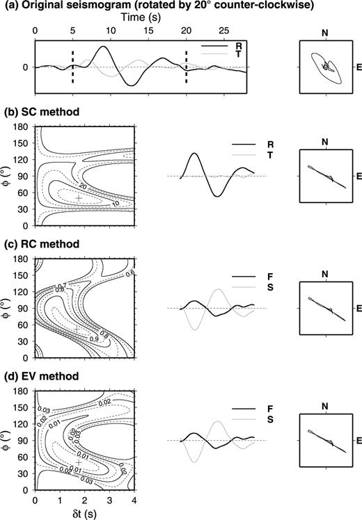
The same content as in Fig. 2, with random noise introduced into the seismograms. Before the splitting measurements, the north and east components were rotated counter-clockwise by θ=−20° to represent correcting the misalignment. After measurement, the best-fitting splitting parameters are φ= 50°, δt= 1.76 s by the SC method in (b), φ= 52°, δt= 1.68 s by the RC method in (c), and φ= 50°, δt= 1.76 s by the EV method in (d).
In Fig. 3, it is noted that the values of φ determined by the RC and EV methods change linearly with θ. This means that the small misalignment angle of the horizontal components only results in a small error in the value of the fast polarization direction (φ) when the RC or EV method is used. On the other hand, the value of φ determined by the SC method non-linearly varies with θ. This means that the small misalignment angle of the horizontal components may result in large error in the value of the fast polarization direction (φ) when the SC method is used. The measurements of the splitting time (δt) remain unaffected by the component misalignment with either RC or EV method; however, a large error will be introduced into the splitting time (δt) due to component misalignment when the SC method is used.
The RC and EV methods are based on the similarity of the fast and slow waveforms in weakly anisotropic media. They allow the linear polarization of the initial undisturbed wave to be out of the ray path plane. However, the SC method assumes that there is linear particle motion of the initial undisturbed wave in the ray path plane, with no energy in the transverse component. If there is component misalignment, there is significant energy in the transverse components after removing the delay time on the slow waves. Hence, the SC method is sensitive to any misalignment of the horizontal components.
3 Comparison with Other Methods
In this section, we compare the GM method with the traditional methods described above. We refer to these traditional methods (SC, RC and EV) without correcting the misalignment of horizontal components before measurement as SC–ST, RC–ST and EV–ST, respectively (ST is abbreviated from seismic station), because they depend on the orientation of the seismic station and assume that there is not the misalignment of horizontal components. In addition, a polarization analysis, such as finding an eigenvector of the eigenvalue calculated for the SKS phase, has been suggested to measure the incoming polarization azimuth and correct the misalignment of horizontal components (Evans et al. 2006). Once this is done, the splitting parameters are measured using the traditional methods. As long as δt0≪T, the initial polarization direction is preserved in the uncorrected particle motion (Vidale 1986). We refer to the traditional methods (SC, RC and EV) with correcting the misalignment of horizontal components before measurement as SC–PL, RC–PL and EV–PL, respectively (PL is abbreviate from polarization analysis), because the angle of misalignment is obtained by the polarization analysis of the SKS phase.
We synthesize an SKS waveform using models with different splitting parameters, and compare these measurements when different misalignment angles (θ0) of the horizontal components are given in models. Random noise is also introduced into the waveform with different S/N ratios. To obtain the average splitting parameters, each measuring method is repeated 40 times using random noise.
Figs 5, S1–S3 show the results of these comparisons. It can be seen that the GM method always results in measurements of the splitting parameters that are close to the models. However, with all other methods (SC–ST, RC–ST, EV–ST, SC–PL, RC–PL and EV–PL), the measurement of the splitting parameters agrees less with the models. The SC–PL results are as good as the GM results in some models (Fig. S1), but the correction of the misalignment of the horizontal components by the polarization analysis of the SKS phase is unreliable. The model test indicates that the error in the radial direction deduced from the SKS phase increases with δt0 of the model and also varies with φ0 or BAZ (Fig. S4). The EV–ST method always gives the correct splitting time δt for different models, and the fast direction φ evaluated by EV–ST varies linearly with θ0 and φ=φ0−θ0. The RC–ST method performs poorly, especially when the BAZ is close to the fast direction φ0 in the model, such as BAZ = 120° and φ0= 110° (Fig. S3).
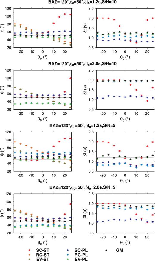
The variation between splitting measurement results (φ and δt) with horizontal component misalignment (θ0) by different methods for the models (BAZ = 120°, φ= 50°). Each value in this figure is the average of 40 results measured from models with different random noise and the error bar represents the STD. The traditional methods, SC–ST (red points), RC–ST (orange points) and EV–ST (brown points), result in measurements with large errors when θ0 is large, due to without correcting the misalignment. The methods SC–PL (dark blue points), RC–PL (light blue points) and EV–PL (green points), result in measurements with large errors when δt0 is large, due to the horizontal orientation defined by the uncorrected particle motion. The GM method (black points) always provides results with small departure from the models.
We also calculate the apparent splitting parameters for two-layer anisotropy models with misalignment of the horizontal components, and compare the GM method with SC–ST, RC–ST and EV–ST. For the two-layer model, we use φlow and δtlow to represent splitting parameters in the lower layer and φupp and δtupp in the upper layer, respectively. The synthetic waveform is generated by a damped sinusoidal signal as the incidence SKS phase with a BAZ. When passing through the lower layer, the waveform splits into two orthogonally polarized quasi-shear waves with the φlow and δtlow; when passing through the upper layer each quasi-shear wave splits into two orthogonally polarized quasi-shear waves with the φupp and δtupp. Four quasi-shear waves are combined to produce the two horizontal components. Fig. 6 shows that the GM method obtains the apparent splitting parameters φapp and δtapp in agreement with the theoretical values, which are calculated by the SC method from a model without horizontal misalignment of components. There are significant deviations between those results from other methods and the theoretical values. We also introduce noise into the two-layer anisotropy models; in those cases, the GM method performs well. The large deviation from the theoretical values and the large standard deviation (STD) only arise periodically at particular BAZ where the theoretical values of the apparent splitting parameters change abruptly (Fig. S5).
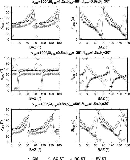
The variation in splitting measurement results (φapp and δtapp) with the BAZ by different methods for two-layer anisotropic models, with the occurrence of horizontal component misalignment (θ0= 20°). Measurements by the traditional methods, SC–ST (diamonds), RC–ST (open circles) and EV–ST (crosses), deviate significantly from the values (black line) predicted by the models. The GM method results (closed circles) almost fit the values predicted by the models.
For the anisotropic structure with either single or double, laterally homogenous, horizontal anisotropy layers, the GM method is valid for measuring the splitting parameters, even with misalignment of the horizontal components caused by sensor misorientation or by heterogeneity at shallow depths. If the radial direction of SKS is deflected an angle −θ from the BAZ by the heterogeneity at a depth greater than the anisotropy zone, the GM method will obtain splitting parameters with an error equal to −θ.
4 The Misalignment of the Horizontal Components at ULN
Station ULN is a permanent broad-band station deployed since 1994 in the City of Ulaanbaatar, Mongolia. A large number of teleseismic waveforms have been recorded, and many SKS splitting parameters have been measured based on these data (Gao et al. 1994; Luo et al. 2004; Liu et al. 2008; Barruol et al. 2008). Results from these studies are inconsistent, mostly due to the different SKS splitting measurement methods and different data processing and selection criteria used by those studies. In Liu et al. (2008), θ= 10° has been used to revise the misalignment of the horizontal components prior to the SKS splitting measurement.
As explained in Liu et al. (2008), there are two possibilities resulting in the misorientation at station ULN. One is that the local magnetic declination at ULN is significantly different from the expected value. Another reason is that the sign of the declination (which is about 3.5–4.67° towards the west from 1995 to 2009 based on data from the Community Coordinated Modeling Centre ) was erroneous, and as a result, the seismometer was rotated by −5° or so counter-clockwise instead of clockwise relative to magnetic north when it was installed.
We selected events occurring at distances greater than 85° with magnitude (Mw) larger than 5.3 over the period 1995–2009. A careful visual inspection of the data allows us to retain seismograms of 31 events with clear SKS phases (Table S1). Most events are located in the southwest of the Pacific.
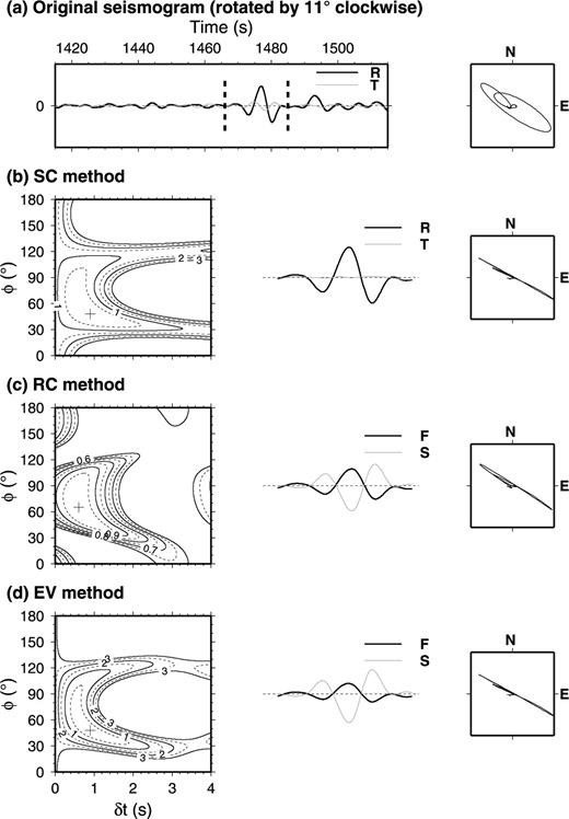
To suppress the potential effects on the splitting parameters caused by noise, we applied a bandpass filter over the dominant frequency of the teleseismic waveforms at 0.03–0.2 Hz. The splitting parameters, φ and δt, were calculated in a window length of about 16 s over the SKS phase at ULN. Fig. 7 shows the 20th event in Table S1 analysed by the SC, RC and EV methods. The results for the optimal pairs of splitting parameters are φ= 42°, δt= 1.8 s by the SC method, φ= 76°, δt= 0.6 s by the RC method and φ= 59°, δt= 0.9 s by the EV method.
SKS splitting measurements by traditional methods at the ULN station form the 20th event in Table S1. After measurement, the best-fitting splitting parameters are φ= 42°, δt= 1.8 s by the SC method in (b); φ= 76°, δt= 0.6 s by the RC method in (c) and φ= 59°, δt= 0.9 s by the EV method in (d). For more explanation see Fig. 1.
Using the GM method, the splitting parameters are calculated with different θ by the SC, RC and EV methods. In Fig. 8, the splitting parameters agree between SC and EV, and the transverse energy reaches a global minimum, at θ= 11°. After the horizontal components are rotated by 11° clockwise, the SC and EV methods obtain the same splitting parameters φ= 48°, δt= 0.9 s (Fig. 9).
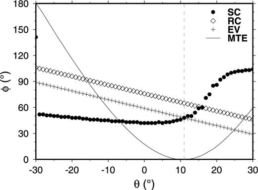
The variation in the fast direction (φ) with the correction angle θ (rotating the horizontal components clockwise). The methods SC (closed circles) and EV (crosses) obtain the same result of φ= 48° when θ= 11°. The transverse energy (thin line) reaches a global minimum at θ= 11°. For more explanation see Fig. 3.
SKS splitting measurements after correcting the horizontal component misalignment at the ULN station form the 20th event in Table S1. The north and east components were rotated clockwise by θ= 11° to represent correcting the misalignment before the splitting measurements. After measurement, the best-fitting splitting parameters are φ= 48°, δt= 0.9 s by the SC method in (b); φ= 65°, δt= 0.6 s by the RC method in (c) and φ= 48°, δt= 0.9 s by the EV method in (d).
Table S2 lists all the measurements of splitting parameters from the events in Table S1. If we neglect the misalignment of horizontal components and measure the splitting parameters using the SC–ST method, the 31 events result in a mean φ of 47 ± 13° and a δt of 1.3 ± 0.5 s. However, if we use the GM method to measure the splitting parameters, the 31 events result in a mean φ of 59 ± 18.8° and a δt of 0.75 ± 0.2 s. The different between the results from the SC–ST and GM methods is 12° and 0.55 s for φ and δt, respectively. In Table S2, θ varies from −3 to 20°, with a mean θ of 8.0 ± 5.3°. It suggests that the misorientation of the sensor is about 8.0°. The large range of the resulting misorientation (from −3 to 20°) implies the heterogeneity at shallower depths beneath station ULN also contributed to the misalignment of the horizontal components. At some temporary broad-band seismic stations, there may be larger misorientation of the sensor caused by installation mistakes, in turn resulting with larger difference between the SC–ST and GM methods.
Gao et al. (1994) obtained φ= 69 ± 6°, δt= 0.7 ± 0.1 s using 3 events; Lou et al. (2004) obtained φ= 45 ± 5°, δt= 1.4 ± 0.4 s using 9 events; Barruol et al. (2008) obtained φ= 51 ± 2°, δt= 0.79 ± 0.03 s using 50 events and Liu et al. (2008) obtained φ= 52 ± 12°, δt= 0.6 ± 0.1 s using 89 events. The comparison of these results is difficult due to the clear azimuthal variations of the splitting parameters as demonstrated in Barruol et al. (2008) and Liu et al. (2008) for this station. Since the averaged splitting parameters are dependent on the azimuthal coverage of the events, whether or not the averages are consistent with previous results is highly dependent on the number of events used.
5 Conclusion
Measurements of the SKS splitting parameters have become popular for studying deformation in the upper mantle, but many factors may lead to false measurements, such as low signal-to-noise ratio, improper bandpass filtering and window length of analysed signals (Vecsey et al. 2008). In addition, misalignment of the station horizontal components may cause false measurements.
Due to local magnetic effects and/or erroneous installation of the sensors, the sensor misorientation may be present at seismic stations. The complex structure in the shallow depths beneath stations is another important factor that can lead to misalignment of the station horizontal components. Because the polarization directions of the corrected SKS phase are out of the ray path plane and differ from the BAZ, misalignment of the horizontal components will result in a false measurement of the splitting parameters by SC methods.
We suggest that a splitting analysis should be repeated with different assumed angles of misalignment (typically ranging from −30 to 30°). The corrected measurement of the SKS splitting parameters should be obtained by meeting two criteria: (1) the horizontal rotating angle is found for the global minimum transverse energy using the SC method and (2) the results from the SC method and the EV method are consistent. Synthetics tests show that the GM method is operative for single- and double-layer horizontal axis anisotropic medium.
Acknowledgments
The IRIS Data Centre kindly provided us with seismogram data. We thank Aimin Du for providing constructive suggestions. Constructive comments are due to Stephen Gao, an anonymous reviewer, and editor Jun Korenaga. This research is supported by grants from the Chinese National Natural Science Foundation (Nos. 40974025 to X. Tian and 40721003 to Z. Zhang) and National Key Project 2008ZX05008-006 to ZZ. All figures were made by using the Generic Mapping Tools software package (Wessel & Smith 1998).
Supporting Information
Additional Supporting Information may be found in the online version of this article:
Figure S1. The variation in splitting measurement results (ø and δt) with the horizontal component misalignment (θ0) by different methods for the models (BAZ = 120°, ø0 = 70°). For more explanation see Fig. 5.
Figure S2. The variation in splitting measurement results (ø and δt) with the horizontal component misalignment (θ0) by different methods for the models (BAZ = 120°, ø0 = 90°). For more explanation see Fig. 5.
Figure S3. The variation in splitting measurement results (ø and δt) with the horizontal component misalignment (θ0) by different methods for the models (BAZ = 120°, ø0 = 110°). For more explanation see Fig. 5.
Figure S4. The error in the radial direction by polarization analysis of the SKS phase. The eigenvector of the maximum eigenvalue calculated by SKS phase is used to measure the incoming polarization azimuth. (a) The error variation with δt0 and different S/N. In these models, the BAZ is given as 120° and ø0 as 60°. (b) The error variation with ø0 for a given δt0. In these models, the BAZ is given as 120. and the synthetic waveforms are noisefree.
Figure S5. The variation in splitting measurement results (øapp and δtapp) with the BAZ by the GM method for two-layer anisotropic models with a horizontal component misalignment (θ0 = 20°). Each value (closed circles) is the average of 40 results measured from models with different random noise (S/N = 5), and the error bar represents the STD. The values predicted by the models are shown by black lines.
Table S1. List of events used to measure SKS splitting at station ULN.
Table S2.SKS splitting measurements at station ULN.
Please note: Wiley-Blackwell are not responsible for the content or functionality of any supporting materials supplied by the authors. Any queries (other than missing material) should be directed to the corresponding author for the article.
References
