3-D shear wave radially and azimuthally anisotropic velocity model of the North American upper mantle Free

Summary

1 Introduction

Seismic anisotropy in the Earth's upper mantle is generally attributed to lattice preferred orientation of anisotropic crystals in minerals such as olivine and pyroxene (e.g. Nicolas & Christensen 1987) resulting from rock deformation in past and present mantle flow. Under continents, seismic anisotropy results from a combination of frozen-in lithospheric anisotropy from past deformation processes, shear coupling between the lithosphere and asthenosphere and current flow in the asthenosphere (Park & Levin 2002). Characterizing seismic anisotropy and relating it to past and present geodynamic processes thus provides insights into our understanding of the driving mechanisms of plate tectonics and lithospheric evolution.

The North American (NA) continent is in many ways an ideal target for this type of study, owing to its rich tectonic history. The central cratonic part of the continent is a mosaic of amalgamated Archean blocks and Proterozoic terranes, and has remained stable since 1 Ga (Hoffman 1989). On the other hand, successive episodes of extension, contraction, and magmatism have reworked the continent and its margins since the formation of its stable core (e.g. Hoffman 1989; Wernicke 1992; Thomas 2006; Whitmeyer & Karlstrom 2007). Also, subduction, extension and strike-slip deformation processes initiated in the late Cenozoic are still active on the continent's western and southwestern margin (e.g. Atwater 1970).

Our knowledge of the NA anisotropic structure comes mostly from studies of core-refracted shear wave (SKS) splitting measurements and surface wave tomographic inversions. The SKS method (e.g. Vinnik et al. 1989; Silver & Chan 1991) provides good lateral resolution for azimuthal anisotropy across the continent, especially in those areas where broad-band station coverage is dense, but depth resolution is poor, and there are trade-offs between the strength of anisotropy and the thickness of the anisotropic domain. Surface wave tomographic inversions can provide constraints on both radial and azimuthal anisotropy (e.g. Montagner & Nataf 1986), and provide better vertical resolution, but they are limited in horizontal resolution due the long wavelength nature of the surface waves. Naturally, the combination of the two types of data can provide better constraints, both vertically and horizontally, on upper-mantle anisotropic structure.

Previously, we developed an approach which combines three-component surface waveforms and SKS splitting measurements and applied it to the study of the NA continent before the USArray Transportable Array (TA) deployment (Marone et al. 2007; Marone & Romanowicz 2007). In Marone (2007; from here on referred to as MR07_1), we inverted long period teleseismic waveforms for a continental scale 3-D model of isotropic shear velocity V_s, and radial anisotropy ξ, Lateral resolution was on the order of 500 km for V_s and 1000 km for the radial anisotropy parameter ξ. In Marone & Romanowicz (2007; from here on referred to as MR07_2), using MR07_1 as starting model, we jointly inverted surface waveform data and SKS splitting measurements for a 3-D upper-mantle model of azimuthal anisotropy. These two studies identified two distinct depth domains of anisotropy that could be associated with the lithosphere and asthenosphere, respectively. In particular, we found that, below a depth that corresponds to the lithosphere–asthenosphere boundary (LAB), the direction of the fast axis of azimuthal anisotropy aligns with the absolute plate motion (APM in HS3-NUVEL-1A; Gripp & Gordon 2002), delineating an LAB with significant depth variations (∼80–200 km) across the continent. In the cratonic part of NA, these results agree with several local scale studies (e.g. Li et al. 2003, 2005; Deschamps et al. 2008; Darbyshire & Lebedev 2009).

In the meantime, a significant number of receiver function (RF) studies at the global (Rychert & Shearer 2009), or continental scale (e.g. Abt et al. 2010; Ford et al. 2010), have failed to detect the LAB under stable parts of the continents at a depth compatible with tomographic inversions, that is, between 180 and 250 km in NA (van der Lee & Nolet 1997a; Marone et al. 2007; Nettles & Dziewoński 2008; Bedle & van der Lee 2009); these results suggest a gradual velocity gradient with depth across the LAB. On the other hand, these RF studies detect a negative velocity jump at much shallower depths (∼100 km), suggesting the presence of a mid-lithospheric boundary (Romanowicz 2009) that could be related to the ‘8° discontinuity’ reported in long range seismic refraction studies (Thybo & Perchuc 1997; Thybo 2006).

Our previous studies (MR07_1 and MR_07_2) focused on first order large-scale features of the continental upper mantle. With five more years of data collected from the recent TA deployment, as well as from many other temporary broad-band networks across the continent, we have significantly augmented both our waveform and SKS splitting data sets. This has allowed us to achieve higher resolution and leads to interesting new observations. In two companion papers, we focused on specific aspects of the azimuthal anisotropy part of our new model: (1) the layering of anisotropy in the cratonic upper mantle, where we can now distinguish three domains of azimuthal anisotropy, two in the lithosphere and one in the asthenosphere (Yuan & Romanowicz 2010a; hereafter referred to as YR10a). In particular, the boundary between the two lithospheric layers roughly corresponds to the negative velocity jump detected in RF studies and (2) the 3-D variations of anisotropy in the most data rich region, the tectonically active western United States (WUS), where the complex SKS splitting patterns observed at the surface can be attributed to relatively simple, but depth dependent patterns of anisotropy (Yuan & Romanowicz 2010b; hereafter referred to as YR10b).

In this paper, we present our complete continental scale 3-D model of isotropic shear velocity, and radial and azimuthal anisotropy, and relate some of the robust features to past and present tectonics. In what follows, we describe our data sets, model parametrization and inversion approach, and present a variety of resolution tests using realistic multiple length scale structures. We show that the radial and azimuthal anisotropy patterns provide complementary information to that of isotropic velocities in recognizing features associated with past lithospheric deformation processes as well as present day shear related to coupling between the lithosphere and asthenosphere.

2 Methods, Inversion Setup and Resolution Tests

2.1 Methods

Following the methodology described in MR07_1 and MR07_2, we consider three component time-domain long period teleseismic waveforms recorded at stations in North America, low pass filtered with a corner frequency of 80 s and a cut-off frequency of 60 s. We compare observed waveforms, divided into wavepackets separating fundamental mode and overtone energy, with synthetic waveforms computed using a normal-mode approach. Both the forward and inverse parts of the analysis are cast in the framework of the non-linear normal mode asymptotic coupling theory (NACT; Li & Romanowicz 1995). NACT takes into account coupling between modes along and across dispersion branches, thus allowing us to represent the body wave character of overtones. The asymptotic formalism collapses the waveform sensitivity to structure onto the vertical plane containing the source and the receiver, resulting in 2-D finite frequency kernels. It is much faster computationally than a complete 3-D Born calculation, and also has the advantage of including multiple forward scattering (Romanowicz et al. 2008). It does not take into account the effect of off-path propagation in the horizontal plane (focusing), but this primarily affects amplitudes and we are modelling the phase part of our waveforms at this stage.

Our goal is to invert for 3-D variations of isotropic, as well as radially and azimuthally anisotropic shear velocity structure, in the upper mantle, inside the region of study. Because our long period waveforms are mainly sensitive to a small subset of the full 21 elements of the anisotropic tensor, following MR07_1 and MR07_2, we parametrize our model in terms of isotropic shear wave velocity (V_s), radial anisotropy parameter ξ= (V_sh/V_sv)², and 2-ψ anisotropic parameters G_c and G_s (Montagner & Nataf 1986). We consider empirical proportionality relations, based on mineral physics experiments at upper-mantle conditions (e.g. Montagner & Anderson 1989) to take into account the weak sensitivity of our waveforms to the other relevant elastic parameters: density, ρ; isotropic P velocity, V_P; radial anisotropy parameters, ϕ and η and azimuthal anisotropy parameters, B_c,s, H_c,s and E_c,s. These relations are as described in Panning & Romanowicz (2006) for the radial anisotropy parameters and in MR07_2 for the azimuthal anisotropy parameters.

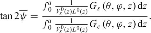
The two azimuthal anisotropy parameters, G_c and G_s, which relate to the local anisotropy strength G and fast axis direction ψ_G at a point (θ, ϕ, z) in the Earth interior as and ψ_G= 0.5 et al. arctan et al. [G_s(θ, ϕ, z)/G_c(θ, ϕ, z) ] (Montagner & Nataf 1986), can also be inferred from body wave SKS splitting measurements (Montagner et al. 2000). Under commonly used assumptions in SKS studies (Vinnik et al. 1989; Silver & Chan 1991), that is, weak anisotropy with a horizontal symmetry axis and long period vertically incident SV waves, it is shown that the accumulated splitting time and apparent fast axis direction at the surface relate to G_c and G_s as follows:

1

where ψ is the backazimuth associated with a radially polarized SKS wave for an event. By removing the event backazimuth ψ, eq. (1) leads to an inversion problem (MR07_2)

2

3

where G_s(θ, ϕ, z) and G_c(θ, ϕ, z) are model parameters to invert for; and are obtained from the splitting data; and defines the sensitivity kernels of the SKS data, by substituting V_s(z) and L(z) with V⁰_s (z) and L⁰ (z) (assuming weak anisotropy) where superscript 0 is for the 1-D reference model.

We jointly invert for the 3-D azimuthal anisotropy structure using the surface wave waveforms and the SKS data in the form described in eqs (2) and (3). In our inversion > and , with the incidence wave backazimuth ψ removed, are the station averaged splitting parameters. After the inversion, these station averaged apparent splitting parameters can be predicted from inverted G_s(θ, ϕ, z) and G_c(θ, ϕ, z) by

4

5

2.2 Augmented waveform data set

Compared to our previous isotropic and radial anisotropy model MR07_1, our augmented data set includes a large number of new waveforms recorded from 2004 January to 2008 December (Fig. 1). For the part of our study region covered by the USArray TA stations up to 2008 December, we used data from these stations, and from permanent stations including the USArray Backbone Array, the United States National Seismic Network (USNSN) and some local permanent networks (e.g. using the IRIS/DMC nomenclature: BK, CI, IW and UW). For regions outside of the TA coverage, we collected data from the Canadian National Seismograph network (CN) and other available regional and local permanent networks (e.g. AK, CN, LD, MX, NE, NM, NR and USNSN), as well as available temporary PASSCAL experiments. We also included some permanent and temporary stations outside, but near the edges of our model area (CU, GE, GLISN, IU, DW, PR, XD and XF), and selected events that effectively sample our model space in azimuth. Waveforms from teleseismic distances (15–165°) were then filtered with 60 and 400 s cut-off frequencies, and individual wavepackets that represent either fundamental mode or overtone phases were weighted by their waveform amplitude, noise and path redundancy as described in Li & Romanowicz (1996).

Figure 1

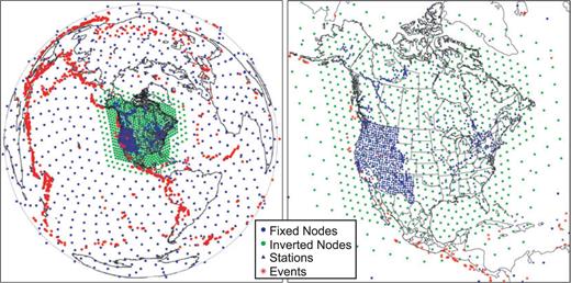
Event and station distribution, and spherical spline nodes used for the model parametrization. Left-hand panel shows the events (red stars) on the global scale, centred on North America (NA). Blue triangles are broad-band stations used. Green dots are the level 6 (∼250 km spacing) and 5 (∼500 km spacing) spherical spline model nodes targeting the study area, for isotropic velocity/radial anisotropy, and azimuthal anisotropy inversion, respectively. Blue dots are the level 4 (∼1000 km spacing) nodes used to correct for the outside 3-D structure, which remains fixed in the inversion. Right-hand panel is a zoomed view for the North American region.

Open in new tabDownload slide

2.3 Station averaged apparent splitting data

The SKS data set used for our previous NA azimuthal anisotropy upper-mantle model MR07_2 was augmented to achieve better lateral coverage, taking advantage of the TA and recent PASSCAL temporary deployments. We consider station-averaged rather than single event SKS measurements to avoid contamination by the possible presence of anisotropy outside of our model space (e.g. the core–mantle boundary region): by station averaging, the incoherent signal along the ray path outside of our model region is effectively muted, while consistent anisotropic signals from the single- or multiple-layered upper-mantle structure within our model space contribute to the apparent splitting measurements at the surface. In addition, most SKS measurements we compiled from recent studies and other groups' compilations (e.g. Frederiksen et al. 2006; Liu 2009; Bastow et al. 2010; Courtier et al. 2010; Eakin et al. 2010) do not provide individual event information. Here, we assume that the station averaged measurements are representative of the true apparent splitting. The general consistency of the SKS splitting directions across neighbouring regions indicates that this is a good assumption at the lateral resolution of the present study.

In a variety of SKS studies, backazimuthal variations have been documented and interpreted in terms of multiple layer anisotropy (e.g. Levin et al. 1999; Polet & Kanamori 2002; Long et al. 2009; Bonnin et al. 2010). If the event data set used to form the station average does not include a large enough backazimuth range, the station-averaged SKS measurements may be biased. It may become useful in the future, for a higher resolution study, to use single event SKS measurements with a slightly modified eq. (1) to account for event backazimuth ψ and incidence.

The formalism we use here (eqs 1–5) relies on the assumption that the periods of the SKS waves are long enough (T > ∼10 s) such that the order of layers with distinct azimuthal anisotropy characteristics does not impact the character of the observed splitting (Montagner et al. 2000). While we do not have direct information on the period-range of some of the measurements we collected from the literature, as much as possible, we try to avoid shorter period SKS measurements and assume that the common period range for the data which we include in our study is 10–30 s. We note that the long period assumption is consistent with the small splitting time assumption made in some commonly used methodologies for measuring splitting (e.g. Vinnik et al. 1989; Chevrot 2000).

The distribution of SKS splitting data is rather uneven across the continent. However, the model parametrization filters out short wavelength variations. We compared inversions obtained using all SKS data versus a smoothed version of the data set, and verified that the resulting models are consistent (see Supplementary Information for more details). From here on the results presented and discussed are based on the complete SKS data set.

2.4 Model parametrization and two-step inversion

We parametrize our model space horizontally in terms of spherical splines (Wang & Dahlen 1995) and vertically in terms of B-splines (Mégnin & Romanowicz 2000). Because our data set is much expanded from that used in MR07_1 and MR07_2, we here consider a 2° horizontal node spacing for V_s and ξ, and a 4° horizontal node spacing for azimuthal anisotropy parameters (G_c and G_s). The vertical node spacing varies from 30 to 70 km in the shallow upper mantle down to the transition zone, while below 660 km the node spacing is 100–150 km, down to 1000 km, the lower limit in depth of our model space.

Inversions for 3-D anisotropic structure were conducted in two steps. First, we inverted our waveform data set for radially anisotropic structure (V_s and ξ; referred to as Step 1 inversion). We chose this parametrization rather than solving for V_sv and V_sh separately, as in MR07_1, to avoid additional uncertainties on the amplitude of the radial anisotropy when dealing with different damping in the inversion of the latter two parameters. Three-dimensional structure outside of the region of interest was corrected for, using NACT, by considering the contribution to the observed seismograms of a recent global radially anisotropic 3-D shear velocity model (Lekic & Romanowicz 2010), developed using the Coupled Spectral Element Method (Capdeville et al. 2002). This new global model used using a different global data set, low pass filtered with the same filter band as in our regional case. The 1-D average V_s and ξ model of Lekic & Romanowicz (2010) was used as starting model in our regional inversion (Figs 3a and b). Note that, in contrast to PREM which was used as a reference in our previous study, this model does not include a 220 km discontinuity. Because our waveforms have limited sensitivity to structure at depths <40 km, crustal corrections were applied using the Crust 2.0 model (Bassin et al. 2000) and an approach (Lekic et al. 2010) that takes into account the non-linearity introduced by the large Moho depth variations in the NA continent.

Figure 3

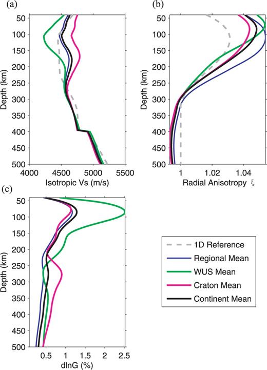
1-D depth profiles of the starting model (which is also the global average; Lekic & Romanowicz, in revision), the NA regional average, and the western US (WUS) average, for variations in isotropic velocity V_s (a), radial anisotropy ξ (b) and azimuthal anisotropy G (c). The craton and continent averages are also shown for comparison.

Open in new tabDownload slide

In the second step (step 2 inversion), after correcting for the effect of 3-D V_s and ξ structure from the previous step 1 inversion, we jointly inverted waveforms and SKS splitting data, for 3-D variations in 2ψ azimuthal anisotropy. We do not apply any a priori starting azimuthal anisotropy model. An iterative least-squares approach (Tarantola & Valette 1982) is applied at each step to solve the inverse problem.

2.5 Resolution tests

A series of resolution tests, focusing the azimuthal anisotropy part of our 3-D model, have been conducted to show the robustness of our joint tomographic inversions for the 3-D NA upper-mantle structure (YR10a and YR10b). From these previous tests we infer that we also are able to accurately recover the distribution of fast axis directions of azimuthal anisotropy down to the transition zone. However, the azimuthal anisotropy strength is systematically underestimated at larger depths (>200 km), particularly so when inverting waveforms only. Our tests show that, while directions of fast axis of anisotropy are very consistent between the two types of inversions, the recovery of azimuthal anisotropy amplitude at depths larger than 200 km is improved by the addition of constraints from the SKS data set (MR07_1,2; YR10a,b).

New synthetics models, which are composed of a wide spectrum of synthetic structures comparable to the inverted model, are tested using the model resolution matrix (e.g. Menke 1989) constructed using the current data set. The new tests confirm the conclusions obtained from similar tests in our previous papers. These new tests show that the resolving power of the augmented data sets is sufficient to recover robust patterns and amplitudes in V_s structure at ∼250 km scale in the first 400 km of the upper mantle. While the patterns of lateral heterogeneity at ∼250 km scale are well recovered in ξ, there is amplitude loss at nearly all depths. Contamination into ξ from V_s and vice versa is in general negligible. Also, both the lateral and depth variations of the fast axis directions of azimuthal anisotropy and its amplitude G are well recovered (at ∼500 km scale) in the upper 200 km. Below 200 km, the fast axis direction is well recovered but G suffers more amplitude loss. However, our tests show that we are able to robustly determine whether the azimuthal anisotropy is concentrated in depth around 300 km or spread over a range reaching transition zone. Details of the resolution tests are found in the Supplementary Information.

3 Inversion Results

As illustrated in the resolution tests from our previous work and this study, the isotropic and anisotropic structure is best resolved above transition zone depths. In what follows, we present the 3-D models, focusing on the upper 500 km of our model space, and discuss their salient features. For reference, geological features that will be mentioned below are shown in Fig. 2.

Figure 2

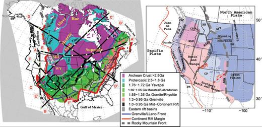
Left-hand panel: Precambrian basement of the North American continent. Precambrian province ages follow Whitmeyer & Karlstrom (2007). The stable cratonic region is defined by the Rocky Mountain Front (grey dashed line) to the west, and the continent rift margin (red thick line) to the east. Labels are: BHT, Buffalo Head Terrane; THO, Trans-Hudson Orogen; MH, Medicine Hat province; WY, Wyoming Province; CP, Colorado Plateau; BC, Baja California. Depth cross-section locations are shown as thick black lines with white circles for better correspondence with Figs 7, 10, 11, 12. Right-hand panel: physiographic provinces of the western US. Labels follow Burchfiel et al. (1992): OM, Olympic Mountains; OCT, Oregon Coast Ranges; CRP, Columbia River Plateau; BB, Belt Basin; IB, Idaho Batholith; HLP, High Lava Plains; ESRP, Eastern Snake River Plain, Sevier T&F, Sevier Thrust and Fold belt; CP, Colorado Plateau; RGR Rio Grande Rift; TR, Transverse Ranges and PR, Peninsular Ranges. Red line demarcates the boundary between the Pacific Plate and the North American (NA), Gorda and Juan de Fuca plates. The thick grey dashed line is the Rocky Mountain Front. Red dashed lines are the two volcanic trends, the Saint George volcanic trend (SGVT) and the Jemez volcanic trend (JVT). The two thin grey lines are the Sevier Thrust and Fold belt, and the Strontium isotope ratio 0.706 line, which, respectively, mark the eastern and western boundaries of the Precambrian passive margin of the continent (Burchfiel et al. 1992). States are labelled as, WA, Washington; OR, Oregon; CA, California; NV, Nevada; ID, Idaho; WY, Wyoming, UT, Utah; CO, Colorado; AZ, Arizona and NM, New Mexico.

Open in new tabDownload slide

3.1 Regional average model

In Figs 3(a)–(c), we present the average 1-D depth profiles for our model region, as well as separate averages for the cratonic part of North America and the tectonically active west. We present two mean profiles, one for the entire region of our study, which includes both continental and oceanic parts, and the other for the continental part only. The continental and regional scale average V_s profiles are similar, and faster than the global average (1-D reference in Fig. 3a) in the depth range 100–200 km, reflecting the contribution of the thick cratonic lithosphere. The craton average is significantly faster than the regional average from the crust down to depths of 250–270 km. This profile shows two minima, one centred around 100 km depth, the other around 250 km, separated by a velocity maximum around 170 km depth. Although the minimum around 100 km depth is not resolved in previous global tomographic studies (Panning & Romanowicz 2006; Kustowski et al. 2008) or regional studies of the NA continent (e.g. MR07_1; Nettles & Dziewoński 2008; Bedle & van der Lee 2009), it is reported at similar depths in recent studies in the Slave craton (Chen et al. 2007) and in most recent global studies of cratons and platforms (Lebedev et al. 2009; Lekic & Romanowicz 2010). In continental Australia, Fichtner et al. (2010) also find that velocities peak at ∼150 km, with a local minimum around 100 km. It has been suggested that this velocity low at 100-km is related to the ‘8° discontinuity’ seen in long-range seismic profiles under continents (Romanowicz 2009). The WUS V_s profile, on the other hand, shows a pronounced minimum between 100 and 140 km depth, followed by a strong positive gradient down to 200 km depth, marking the bottom of the low-velocity zone (LVZ). The profiles converge below 270 km to values that are slightly slower than the global 1-D reference down to transition zone depths. Because we have poor resolution in the first 40 km of the mantle due to the long period character of our waveforms, we cannot resolve a maximum in V_s associated with the thin lithosphere in the WUS.

The ξ profiles (Fig. 3b) show much stronger radial anisotropy than the global average down to ∼250 km depth, and particularly so in the WUS, where ξ peaks at a depth of ∼70 km, much shallower than in the global average, joining the latter below ∼170 km. In the craton, the zone of increased ξ is broader and less pronounced in strength, but persists down to about 300 km. Below that depth, both craton and WUS have slightly ‘reversed’ξ anisotropy (ξ < 1) whereas the global average is isotropic. Interestingly, unlike for V_s, the regional average for ξ is distinct from the continental average and shows a maximum at about 120 km, close to the location of the maximum in the reference 1-D model, but the strong radial anisotropy extends to greater depth than in any of the other profiles. The large ξ between 100 and 200 km comes from the border regions in the Pacific and Atlantic oceans, as also reported in other studies in the Pacific Ocean (Nettles & Dziewoński 2008), and beneath the Coral and Tasman Seas in Australia (Fichtner et al. 2010), reflecting well developed asthenosphere under ocean basins.

Compared to radial anisotropy, the profiles of azimuthal anisotropy strength (G) show much more structure with depth (Fig. 3c). The strongest azimuthal anisotropy is under the WUS and is confined primarily to the first 150 km of the upper mantle. Between 150 and 250 km depth, G is stronger in the WUS than in other parts of the continent. In contrast, under the craton, the G profile has two maxima, around 80–100 km depth, and around 270 km depth. There is also a marked minimum in G around 200 km. As has been discussed in YR10a and will be discussed further below, the minimum at ∼200 km can be associated with the bottom of the lithosphere. Thus the G profile under cratons defines two domains with different average G strength in the lithosphere (∼50–120 km and ∼120–200 km) and a zone of increased G in the asthenosphere (∼200–350 km), possibly tapering off into the transition zone. Based on our resolution tests (Figs S12 and S13), the maximum at 270 km is well resolved in our data, although its amplitude may be underestimated and its exact position in depth is not constrained to better than 50 km. However, we suggest that this maximum at 270 km in the craton and the maximum at ∼80–100 km in the WUS both express the presence of strong horizontal shear related to plate motion in the vicinity of the LAB. The fact that the fast axis direction of azimuthal anisotropy is roughly parallel to the APM everywhere below the LAB, as we will see below, strengthens this argument.

3.2 Isotropic V_s model

Our 3-D isotropic velocity model of the NA continent (Fig. 4) shares many common features with other recent large scale regional shear wave tomographic (van der Lee & Nolet 1997a; Frederiksen et al. 2001; MR07_1; Nettles & Dziewoński 2008; Sigloch et al. 2008; Bedle & van der Lee 2009; Burdick et al. 2009). The spatial similarities among the different models indicate that the first order V_s features found are robust.

Figure 4

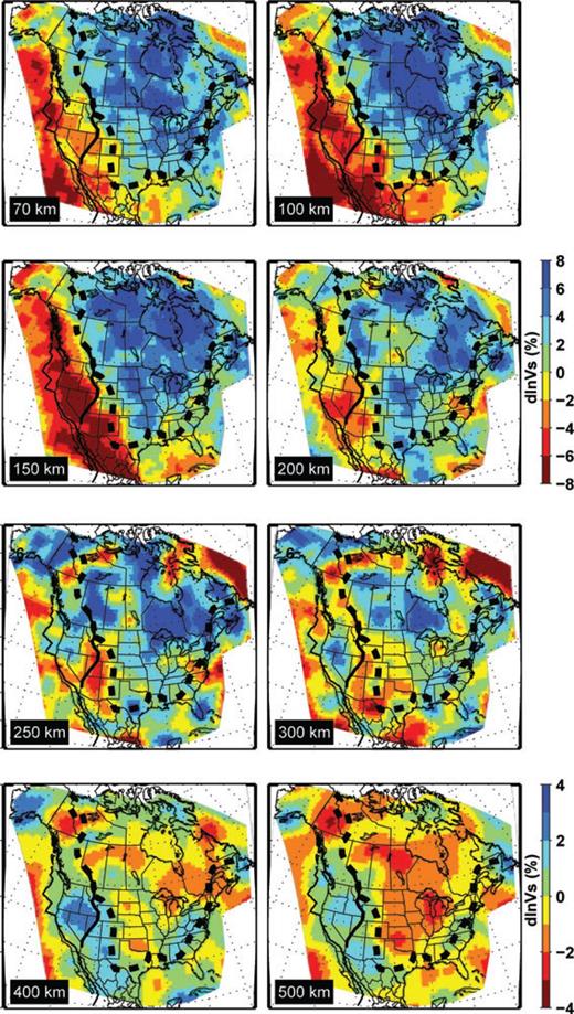
Isotropic velocity (V_s) perturbations, plotted with respect to the NA regional average shown in (Fig. 3). Black dashed line approximately delineates the continent cratonic region, which approximately follows the Rocky Mountain front (RMF) to the west, and the Ouachita and Appalachian fronts to the south and east. Velocity variations are saturated at –8 to 8 per cent scale at ≤200 km depth, and –4 to 4 per cent below 200 km. The Palaeozoic continent rift margin in the western US, which spatially correlates with the Sevier thrust and fold belt in the western US, is shown as a black line for reference.

Open in new tabDownload slide

At shallow depths (i.e. <200 km) the NA continent is dominated by fast velocities under the stable cratonic regions, and slow velocities in the tectonically active WUS. In the west, the sharp transition between the two domains closely follows the Rocky Mountain Front (RMF), and in the east, the Ouachita Orogen and the Appalachian Orogen (broken lines in Fig. 4). In the Precambrian regions, the fast velocities extend below 200 km depth, except for a trend of slow velocity at about 200 km beneath the Great Fall Tectonic zone in north Wyoming province and beneath the Trans-Hudson Orogen separating the Superior and Hearne provinces to the north. This slow velocity anomaly is spatially associated with an upper-mantle low-conductivity zone revealed from electromagnetic inversions (Jones et al. 2005) and a cylindrical like low velocity anomaly from a local body wave traveltime inversion (Bank et al. 1998). In the depth range 150–250 km, large low velocity anomalies are associated with the Basin and Range and the East Pacific Rise (EPR).

Above 200 km, velocities on the continental margins show much larger spatial variations. At the southwestern edge of our model, in the Pacific Ocean and under the Pacific Plate, velocities are very low in the depth range 70–150 km (<–6 per cent with respect to the regional average). At 150 km depth, this anomaly connects to the EPR. Slow velocities are also present beneath the Juan de Fuca (JdF) and Gorda plates, albeit in a narrower depth range (70–100 km). This whole system of low velocities seems to be connected from south (EPR) to north, through the Basin and Range and into the JdF and Gorda ridge system. This is best seen in a 3-D rendering of the velocity structure in the WUS as presented in Figs 5(a) and (b). The Gulf of Mexico, on the other hand, is generally slow above 150 km, while below that depth, a fast anomaly is present and extends into the centre of the continent. In the eastern offshore border of the US, which corresponds to the >100 Ma old north Atlantic part of the NA Plate, fast velocities are present down to at least 100–150 km. Further north, the velocity is slow beneath the extinct Labrador Sea rift system down to 300 km depth.

Figure 5

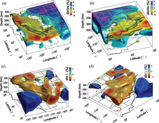
3-D rendering of the isotropic V_s and radial anisotropy model viewing from the southwest (a and c), and from the northwest (b and d). The isosurfaces in (a) and (b) are drawn at –1.5 and 3 per cent for the slow and fast velocities, respectively. The velocity variations are with respect to the NA regional average. For radial anisotropy (c and d), the isosurface values are −2 and 4 per cent. Green lines at the top of each plot show the western US physiographic regions. Thick black line shows the plate boundary between the North American and the Pacific plates.

Open in new tabDownload slide

The most striking feature in the tomographic V_s maps is the sharp boundary between the fast and slow velocities across the RMF (Figs 4, 5a and b). Except for small perturbations at shallow depths (∼100 km) beneath the Rio Grande rift system, the location of this craton-to-active-WUS transition closely follows the east side of the Laramide deformation front which roughly follows the RMF. Thinning of the cratonic lithosphere towards the WUS is confined between the Laramide front and the Strontium ratio 0.706 line (Armstrong et al. 1977) between the Columbia River Plateau/High Lava Plains and the Belt Basin, and between the Idaho Batholith and the eastern Snake River Plain to the north side; the portion of the Sevier Thrust and Fold front from the Eastern Snake River Plain to the Colorado Plateau; and along the central to eastern Colorado Plateau further south (Figs 2 and 4). As seen in some smaller scale studies (e.g. Dueker et al. 2001; Obrebski et al. 2010), we observe three fingers of low velocity penetrating in a southwest–northeast direction into the craton, and roughly corresponding to zones of Cenozoic volcanism, beneath the Snake River plain, beneath the Saint George and Jemez volcanic trends (see Fig. 2 for locations). This is most prominently seen in our model at a depth of 100 km (Fig. 4).

Between 200 and 250 km depth, the sharp boundary between the fast and slow velocities across the RMF disappears. Significantly faster velocities are present under the Archean Superior province, the Palaeo-Proterozoic Buffalo Head terrane in northern Alberta, and the Archean Rae province. Under Alaska, high velocities appear in this depth range, and extend deeper into the transition zone, likely related to the Alaskan subduction. Large slow velocities are present under the Labrador Sea, northeastern Pacific, and the Rio Grande rift system. In the WUS, fast velocities associated with the subducted JdF slab are present beneath Washington, Oregon and Nevada below 250 km. In the transition zone, fast velocities associated with the sunken Farallon slab (van der Lee & Nolet 1997b) are present under Arizona and New Mexico, and extend further south into Mexico (e.g. Figs 4 and 5b).

3.3 Radial anisotropy ξ model

Under most of the study area, as in the global average, ξ > 1 down to 300 km depth (Fig. 3b), reflecting the presence of the top boundary layer, dominated by horizontal shear, in the global mantle convection system. We first show the absolute ξ (i.e. with respect to isotropy) in map view (Fig. 6). The large-scale features are similar to those of our previous model MR07_1, that is, widespread dominantly positive ξ at depths shallower than 200 km under the oceans and the stable part of the continent. The main departure from this trend is the negative dlnξ present in the WUS, starting at 150 km, and likely associated with JdF subduction, the Rio Grande rift, Basin and Range and the EPR to the south, which appear to form a quasi-continuous system reflecting a component of vertical flow, as best seen in the 3-D rendering in Figs 5(c) and (d).

Figure 6

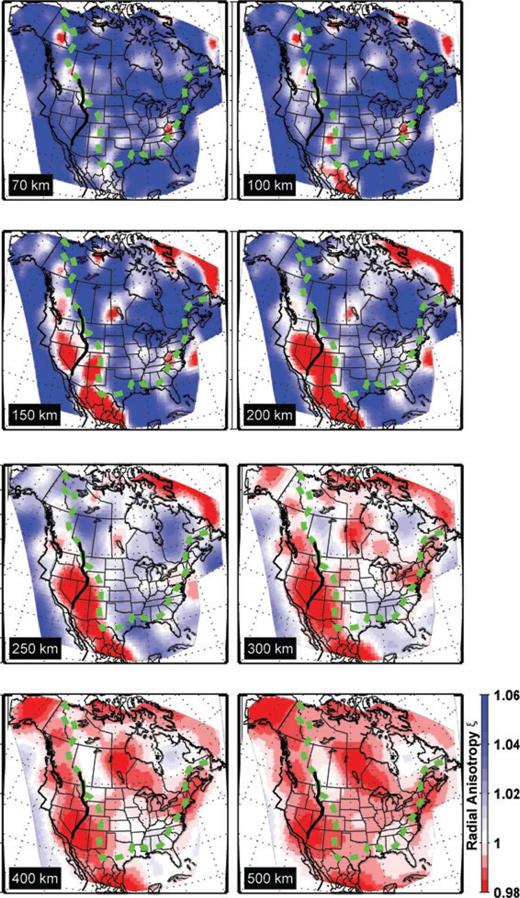
Radial anisotropy parameter ξ= (V_sh/V_sv)², plotted with respect to isotropy. Green dashed line approximately delineates the continent cratonic region, as in Fig. 4. Colour scale is the same for all depths. The Sevier Thrust and Fold belt in the western US is shown as a black line for reference.

Open in new tabDownload slide

Many secondary small-scale negative dlnξ anomalies are also robust, as indicated from our synthetic tests (Figs S2–S5). At shallow depths (70–100 km), these negative anomalies correlate with surface geological features: for instance, along the RMF in the western Cordillera; under the Rio Grande rift in central Colorado; and along the rifted continent margin in the south and southeastern US. Many negative dlnξ anomalies are also seen at shallow depths (<250 km) at several locations along the Trans-Hudson Orogen (THO); the most prominent one is located at the eastern boundary of the Sask craton (Fig. 2), which is entirely in the THO, and is spatially accompanied by slow velocities (Fig. 4). This feature coincides with a quasi-cylindrical low velocity feature which is interpreted as resulting from either mantle plumes or asthenospheric instabilities in Bank et al. (1998). At larger depths (>250 km), the WUS exhibits a negative d ln ξ anomaly which continues into the transition zone.

3.4 The Colorado Plateau

The Colorado Plateau stands out as a unique feature. It is separated from the stable cratonic region to the east by the Rio Grande rift (Fig. 4). Compared with the very slow velocities to the west in the Basin and Range, the lithosphere of this relatively fast velocity block is thin in its southern portion (∼70 km) and thickens to >150 km in the central and northwestern part of the Plateau, as best seen in cross-section view (Fig. 7). The mean olivine composition calculated from xenolith samples at the Four Corners area in the centre of the Plateau gives per cent Fo > 92 down to ∼140 km (Griffin et al. 2004). According to Griffin et al. (2004), the corresponding high magnesium olivine in the Plateau root helps support its high altitude. The 140 km root thickness estimated from the thermobarometric analysis is consistent with our seismic results. In the WUS, the LAB (dashed line in Fig. 7) is measured based on combined observations of reduced isotropic velocity, vertical gradient and/or peak value in the radially anisotropic components of our velocity model, and the S-wave RF measurements of Abt et al. (2010) (see Supplementary Information). The tilting of the LAB to larger depths towards the Northwest is also inferred from body wave tomography images (Sine et al. 2008), and the RF LAB thickness of the WUS in the region (A. Levander, personal communication, 2009). The S-wave RFs of Abt (2010) do not sample the Plateau, but indicate much thinner lithosphere beneath the Basin and Range in agreement with the velocity model (Fig. 7), taking their respective scales of lateral resolution into account. At the northern end of the Plateau, the lithosphere is thick (down to ∼180 km) under the southern edge of the Archean Wyoming province. This also agrees with the 170 km depth estimated from xenolith data for the lithosphere thickness in the (Wyoming/Colorado) State Line district (Griffin et al. 2004). A local P- and S-body wave tomographic study also reveals a north-dipping high velocity structure down to ∼200 km beneath the Wyoming/Colorado border, interpreted as a relic slab segment from the Proterozoic (Yuan & Dueker 2005). The eastern border of the Plateau is significantly intruded by the low velocity and negative ξ feature associated with the Oligocene Rio Grande rift. This result is consistent with GPS velocities that indicate that only the centre of the Colorado Plateau behaves as a stable block and that extension is modifying its eastern (and western) margins (Kreemer et al. 2010). The cross-sections in Fig. 7 show that the low velocity anomaly beneath the lithosphere is tilted to the west and reaches down to >250 km under the western edge of the Plateau, joining, at larger depths, a much broader negative ξ region under the whole WUS (Figs 5c and d). An eastward and upward flow from beneath central Nevada is proposed in geodynamic modelling (Moucha et al. 2008; Moucha et al. 2009) to explain the northeastward shift of the uplift of the Plateau, and the migration of volcanism to the east in the western Colorado Plateau during the past 5 Ma. This view agrees with our V_s and ξ models, but is in contradiction with the idea of a passive rift (e.g. Wilson et al. 2005).

Figure 7

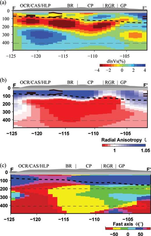
Isotropic velocity V_s (a), radial anisotropy ξ (b) and azimuthal anisotropy fast axis direction (c) cross-sections along FF′ (see Fig. 2 for location of the profile). V_s is plotted with respect to the western US average in Fig. 3. For anisotropy fast axis direction, north is 0°, east is 90° and west is –90°. Labels follow Fig. 2: OCR, the Oregon Coast Range; CAS, Cascades; HLP, High Lava Plain; BR, Basin and Range; CP, Colorado Plateau; RGR, Rio Grande rift; and GP, Great Plains. Thick black (in a, b) green (in c) lines are the LAB estimates from receiver functions with 2σ error bars.

Open in new tabDownload slide

3.5 Azimuthal Anisotropy model

Azimuthal anisotropy shows a strong depth dependence under both the Precambrian regions and the active WUS. This has been discussed extensively in two other papers (YB10a and YB10b). In Fig. 8(a), we present lateral variations in the azimuthal anisotropy strength as defined in Montagner & Nataf (1986), at several depths in the upper mantle, and in Fig. 8(b), the corresponding fast axis directions.

Figure 8

Maps of: (a) Variations of azimuthal anisotropy strength G. (b) Depth dependent fast axis direction. Red arrows show the APM direction (HS3-NUVEL 1A; Gripp & Gordon 2002) of the North American Plate, and blue arrows are those for the Pacific Plate APM. For comparison, the NNR-NUVEL-1A (DeMets et al. 1994) APM directions for the NA and Pacific plates are plotted as green arrows at 250 km depth in (b). Green and grey dashed line approximately delineates the continent cratonic region as in Fig. 4.

Open in new tabDownload slide

The strongest azimuthal anisotropy is found in the WUS between depths of 70–100 km. In most of this region, the fast axis direction is parallel to the NA and JdF APM, except in the southernmost and westernmost part of the region (off-shore) where it is parallel to the Pacific APM, and where strong anisotropy continues down to 150 km. Below that depth, G drops rapidly, and the direction of the fast axis becomes parallel to the Pacific APM. Note that, at 150 km depth, the Colorado Plateau stands out as a region of weak azimuthal anisotropy.

East of the RMF, and throughout most of the NA craton, azimuthal anisotropy is stratified, with two distinct layers in the lithosphere and a deeper layer in the asthenosphere (depths > 250 km) where the direction of fast axis becomes subparallel to the NA APM. This has been discussed extensively in YR10a. Noteworthy is significant azimuthal anisotropy present at 70–100 km depth under the Archean Superior, Slave, Hearne provinces and associated Palaeo-Proterozoic terranes in western Canada. The Proterozoic terranes in the central and eastern US, and the southwestern Superior, however, have very small azimuthal anisotropy strength. The large G in the craton drops in amplitude between 100 and 200 km depth, except for patches of large G in the central US. Below 200 km, G increases again in a broad region between the RMF and the eastern rifted continent margin, and the fast axis direction generally aligns with the NA APM, reflecting shear related to present-day plate motions at and below the LAB.

At 250 km depth, Fig. 8(b) also shows the APM directions calculated for the NA and Pacific plates using the no-net-rotation NNR-NUVEL 1A model (DeMets et al. 1994). For the cratonic region east of the RMF, the NA APM direction in the no-net-rotation frame (green arrows) differs from that in the hotspot reference HS3-NUVEL 1A model (red arrow), especially in the east of the craton. The fast axis direction in the craton is in better agreement with the hotspot frame NA APM. This is also seen in Fig. 9(a), which shows histograms of the angular differences between the fast axis direction and the APM directions for the two reference frame models over the NA craton. West of the RMF, the two APM directions computed for the Pacific Plate are very similar and both are compatible with the fast axis direction in the depth range 150–400 km, as shown in Fig. 9(b). In what follows, we explore in detail the nature of the layering of the upper-mantle anisotropy throughout the NA continent, specifically focusing on several depth cross-sections, along profiles indicated in Fig. 2.

Figure 9

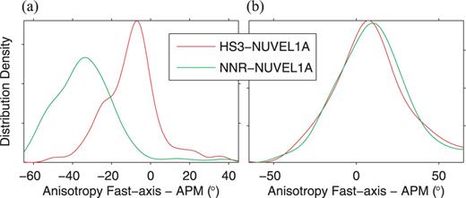
Angular difference between the fast axis direction in our azimuthal anisotropy model and the absolute plate motion (APM) direction from the two models (HS3-NUVEL 1A and NNR-NUVEL 1A), for (a), the cratonic region within the thick dashed line in Fig. 8 and (b), the tectonically active region west of the Rocky Mountain Front. For (a), the APM is that for the North American Plate, while for (b), it is that of the Pacific Plate.

Open in new tabDownload slide

3.6 Depth cross-sections across the continent

In Figs 10 and 11, we present two representative west–east and SW–NE depth cross-sections across the continent, combining information on V_s, ξ and azimuthal anisotropy direction and strength. Two other cross-sections are shown in Figs S15 and S16.

Figure 10

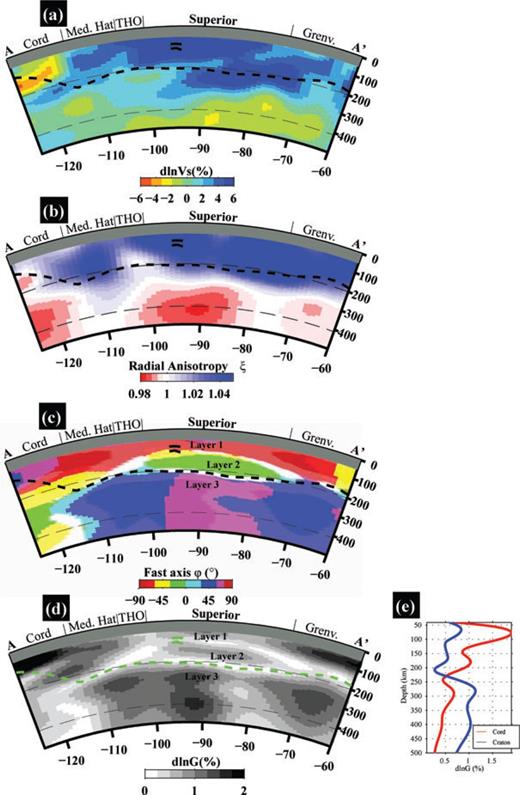
Depth cross-section along AA′, for variations in isotropic velocity V_s (a), radial anisotropy ξ (b), azimuthal anisotropy fast axis direction (c) and its strength G (d). (e) Mean depth profiles for the anisotropy strength for the Cordillera and the craton region, defined, respectively, as west and east of longitude –115°. Thick dashed line is the inferred LAB depth. Labels follows Hoffman (1989), Burchfiel et al. (1992) and Whitmeyer & Karlstrom (2007) and are found in Fig. 2: Cord., Cordillera Orogen; Med. Hat, Archean Medicine Hat province; THO, Proterozoic Trans-Hudson Orogen; Grenv., 1.1 Ga Grenville Orogen. Layering in the cratonic lithosphere and asthenosphere is indicated as Layer 1, 2 and 3. Thick black (in a–c) green (in d) lines are the LAB estimates from receiver functions with 2σ error bars.

Open in new tabDownload slide

Figure 11

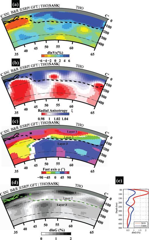
Depth cross-section along CC′, for variations in isotropic velocity V_s (a), radial anisotropy ξ (b), azimuthal anisotropy fast axis direction (c), and its strength G (d). (e) Mean depth profiles for the anisotropy strength for the western US and the craton region, defined, respectively, as west and east of latitude N45°. Thick dashed line is the inferred LAB depth. Labels are: SN, Sierra Nevada; B&R, Basin and Range province; ESRP, Eastern Snake River Plain; GFT, Great Fall Tectonic zone; THO, and Trans-Hudson Orogen. Layering in the cratonic lithosphere and asthenosphere is indicated as Layer1, 2 and 3. Thick black (in a–c) and green (in d) lines are the LAB estimates from receiver functions with 2σ error bars.

Open in new tabDownload slide

In the cratonic lithosphere east of –110°E (Fig. 10c) and north of 45°N (Fig. 11c), we note the presence of two layers of azimuthal anisotropy with different fast axis directions, as shown and discussed in YR10a. Layer 1 and 2 are mostly present under the Archean cratons and the associated mosaic of Proterozoic arcs. The shallow Layer 1 has a general NE–SW to E–W fast axis direction, a direction that is coincidentally parallel to the NA APM. Close inspection shows, however, that this direction is also parallel to the structural trends at the surface: for example, the dominant NE–SW trend of the suture zones in the cratonic region, and the E–W trend in the western and central Superior craton (Percival et al. 2006; Whitmeyer & Karlstrom 2007; also see Fig. 8b at 70 km). In the northeastern Superior province, where the two surface structural zones associated with the New Quebec and the Torngat Orogens trend NW, the fast axis of Layer 1 is also in the same NW direction (Fig. S15c). Layer 2 exhibits a generally north–south to NW–SE direction, and is present beneath Layer 1 under the cratons. Notably, in the Proterozoic arc terranes in the central US, Layer 2 extends to much shallower depths (Fig. S15c), where Layer 1 is missing or very thin. Layer 3 lies below 180–240 km depth, and has a uniformly NE–SW direction that is subparallel to the APM direction of the NA continent (Gripp & Gordon 2002).

The transition between Layer 2 and Layer 3 occurs between 180 and 240 km in the stable continent, in a depth range that falls consistently within the range of lithosphere thickness estimated from seismic, petrologic, electrical and geothermal inversion studies (Jones et al. 2001; van der Lee 2002; Griffin et al. 2004; Moorkamp et al. 2007; Artemieva 2009; Eaton et al. 2009; Miller & Eaton 2010). Notably, in Layer 3, the fast axis direction is everywhere subparallel to the NA APM. We therefore define the anisotropic boundary between Layer 2 and 3 as the LAB in the stable continent. Note this definition of the LAB locates below the peak of the isotropic velocities V_s and radial anisotropy ξ (Figs 3a and b) and falls in a zone of negative V_s and ξ gradient with depth. The LAB thus defined in the craton is indicated by a broken line in Figs 10 and 11.

We note the increased strength of azimuthal anisotropy (G) below 250 km (Fig. 8a), reaching a broad maximum around 270 km, which is also consistent with the 180–240 km LAB estimates, if the increasing G represents the strong horizontal shear between the NA Plate and the underlying asthenosphere. While the precise location of this maximum with respect to the LAB is beyond the resolution of our data set and approach, our resolution tests (Figs S13 and S14) show that we can perhaps distinguish between a concentrated zone of strong azimuthal anisotropy versus one that might be uniformly spread over 250–500 km. Still in the craton, the LAB generally corresponds to a zone of maximum negative gradient in ξ (Figs 10b and 11b), but the locus of minimum radial anisotropy is at somewhat greater depth (by about 30–50 km), also suggesting the presence of a zone of horizontal shear extending into the asthenosphere. The S-wave RFs of Abt et al. (2010) show that, below the US and southern Canadian craton, the RF signal is weak in this depth range, in agreement with a gradual velocity change with depth, and a primarily thermal origin for the LAB.

While ξ > 1, predominantly, in the cratonic lithosphere, we note prominent patches of ξ < 1 in the lower lithosphere under the Archean Sask and central THO (Figs 10b and 11b) which may be related to reworking of the original Archean blocks during the Trans Hudson Orogeny (Dahl et al. 1999; St-Onge et al. 2007), and may further suggest that structural heterogeneities inherited from the old craton building processes may extend deep in the lithosphere, and have been preserved since they were originally emplaced.

In the WUS, on the other hand, it is not possible, with our current data set, to define the LAB based on changes in the fast axis direction of anisotropy, because the lithosphere is thin and young, and there may not be such a transition. Indeed, the frozen-in anisotropy in the lithosphere may either have formed in the present day tectonic regime, or have been destroyed partially during the subsequent tectonism of flat Farallon subduction (Humphreys et al. 2003), so that, to first order, it may be too weak to be detected from the overwhelming large anisotropy underneath, which peaks at 100 km and has the NA APM parallel fast axis direction (Panel d in Figs 10–12) and is proposed to result from strong plate–asthenosphere coupling in the WUS. We note that, in this region, inspection of the V_s and ξ profiles reveals a rather fast drop in V_s and ξ at depths ranging from 70 to 120 km. This depth range falls within or close to the 2σ error bounds on the depth of the largest negative velocity jump found in S-wave RFs (Abt et al. 2010; Figs 7, 10–12). Therefore, in the WUS, RF analysis (e.g. Abt et al. 2010), where it exists, is broadly consistent with our estimates, and the relatively minor discrepancies are easily explained by the different sampling and resolution of the LAB provided by long period waveforms and the S-wave RFs. We stress that in the western parts of the continent, our definition of the LAB (see Supplementary Information) corresponds quite well with the rapid change with depth from fast to slow isotropic velocities and ξ (Figs 10a, 11a and 12a). In the craton, on the other hand, this change is more gradual and, as argued in YR10a, it is more difficult to define the LAB precisely based on either isotropic velocity tomography alone or RFs. Across the RMF, the transition from thin to thick lithosphere is quite rapid, as seen in the V_s and ξ profiles (Figs 10 and 11). This sharp transition is beyond the lateral resolution of our azimuthal anisotropy model, and the LAB estimates across the RMF will need to be revisited in a future higher resolution study.

Figure 12

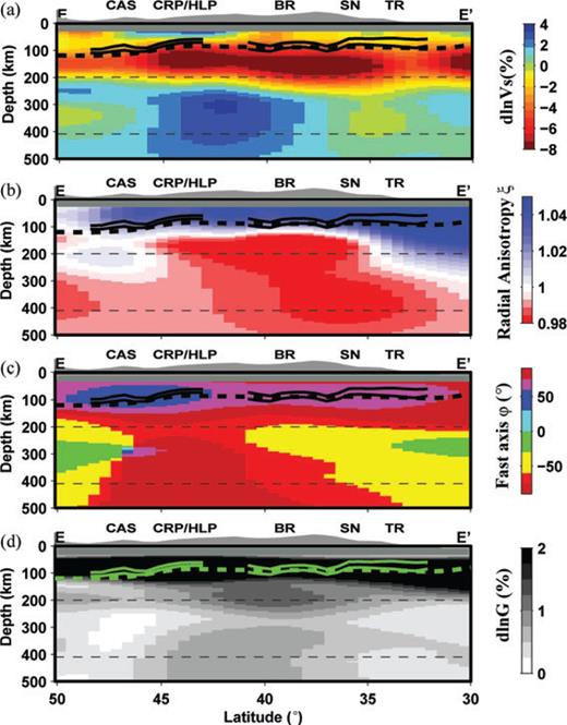
Western US depth cross-sections along EE′ for variations in isotropic V_s (a), radial anisotropy ξ (b), azimuthal anisotropy fast axis direction (c) and its strength G (d). This cross-section also follows the receiver function profile GH in Abt et al. (2010). Two green lines show the averaged and interpreted receiver function LAB estimates with 1σ error bars. Labels are found in Fig. 2: CAS, Cascades; CRP, Columbia River Plateau; HLP, High Lava Plains; BR, Basin and Range; SN, Sierra Nevada; and TR, Transverse Ranges. Thick black (in a and b) and green (in d) lines are the LAB estimates from receiver functions with 2σ error bars.

Open in new tabDownload slide

Unlike in the cratons, where anisotropy layering seems to be relatively simple, at least at the large wavelengths of our study, the WUS upper mantle appears anisotropically complex. Note that, in contrast to the central part of the continent, we are mostly looking at structures below the LAB. As discussed in detail in YR10b, these structures reflect different lateral and depth-dependent domains associated with complex past and present dynamics, as illustrated in a WUS profile in Fig. 12: plate shear (at the shallower depths), manifested by APM parallel fast axis of anisotropy (Fig. 12c), as already discussed; on-going spreading from the EPR to the Basin and Range, as manifested by ξ < 1 in the depth range 100–300 km under much of the profile (Fig. 12b) and the presence of the subducted slab in the north, as manifested by fast velocities in the depth range 250–500 km (Fig. 12a).

A rapid change of the fast axis direction is present at depths greater than 150 km in the WUS upper mantle (Fig. 12c) and is associated with a rapid change in V_s and ξ with depth. We suggest that this marks the bottom of the strong zone of coupling between the lithosphere and asthenosphere. Below this depth, patterns of anisotropy reflect other aspects of mantle dynamics.

Below the LAB across the entire continent, we note alternating regions of pronounced ξ < 1 and of ξ∼ 1 (weak radial anisotropy) with a wavelength of about ∼2000 km, which are associated with slight changes in the direction of the fast axis of azimuthal anisotropy (Figs 10, 11, S15 and S16). This striking quasi-periodicity may be indicative of the presence of small scale convection under the continent. The regions with pronounced ξ < 1 also correspond to regions where faster than average V_s is present at asthenospheric depths. Investigating this in detail would require combining radial and azimuthal anisotropy into a 3-D model of anisotropy with a tilted axis of symmetry, which is beyond the scope of this paper.

4 Discussion

If, as we propose, the transition from Layer 2 to Layer 3 in the craton represents the LAB, the discontinuity between Layer 1 and 2 thus represents a mid-lithospheric feature (Abt et al. 2010; YR10a). As discussed earlier, in the shallow Layer 1, the fast axis direction is parallel to the surface geological sutures, while in the deeper Layer 2, it is generally oriented north–south to NW–SE. The anisotropy strength G (Figs 3c and 8a) associated with Layer 1 is generally larger than in Layer 2, especially under the Proterozoic Wopmay and the western Archean Slave provinces, the western Archean Superior province, and the Trans-Hudson Orogen on its west and northwest sides. The Layer 1 thickness associated with these large values of G is accordingly larger than in other regions (YR10a).

The RF study of Abt et al. (2010) shows the presence of a mid-lithospheric discontinuity (MLD) in the cratonic region. A prominent negative S RF phase is observed at ∼100 km in the southern Superior craton (Figs 10, S15 and S16). At the cratonic scale, such a prominent negative phase in a similar depth range is also found from RF studies at several sparse locations across the NA craton (Yuan et al. 2006; Moorkamp et al. 2007; Snyder 2008; Rychert & Shearer 2009; Abt et al. 2010; Miller & Eaton 2010). An anisotropic transition is also inferred from some RF studies (Bostock 1998; Snyder et al. 2004; Snyder 2008). Upper-mantle high-conductivity layers are observed at ∼100 km beneath the Slave and western Superior cratons (Craven et al. 2001; Jones et al. 2005), showing a change of upper-mantle rock resistivity at this depth. Furthermore, petrologic evidence also supports a change of lithospheric lithology in the cratonic lithosphere in that depth range (Griffin et al. 2004; fig. 2c in YR10a). Coincidence between our Layer 1/Layer 2 boundary and the boundary found in other studies strongly suggests the cratonic lithosphere layering is widespread. Note that the velocity minimum found around 100 km in our cratonic profile appears to be a characteristic of all cratons, as shown at the global scale using clustering analysis by Lekic & Romanowicz (in revision).

While an MLD within the thick cratonic lithosphere is clearly resolved in the model presented here and in S-wave RFs, its relationship to the LAB at the margins of the cratonic lithosphere requires further study. For example, although S-wave RFs have resolved fragmentary discontinuities near the margin of the craton (e.g. the feature at latitude of 45° in Fig. 11) continuous RF imaging of this feature is still lacking. In addition, some ambiguity remains in the exact location of the LAB and the lateral edge of the thick lithosphere. For example, is the RF discontinuity at 45° within thick cratonic lithosphere (as suggested by the interpreted LAB indicated in Fig. 11)? Or is it a shallow LAB next to cratonic lithosphere with a very steeply dipping margin? These questions also apply to the similar feature near the eastern margin of the craton (the feature at longitude of –80° inFig. S16). Determining whether the MLD intersects the LAB at a high angle, asymptotically approaches the LAB, or fades in amplitude towards the edge of the craton would shed light on its origins.

One question associated with our joint waveform and SKS data set inversion is how much the SKS data set contributes to the 3-D azimuthal anisotropy structure. In Fig. 13, we compare the two azimuthal anisotropy models, inverted using the joint waveform only and the joint waveform and SKS data set, respectively. In selected regions of the continent where SKS measurements are present, both models reveal a rather consistent upper 200 km anisotropy structure. The region averaged fast axis directions and anisotropy strength do not vary much whether or not the SKS data set is used. Below 250 km, while the fast axis direction is consistent between the two models in the cratonic regions (a maximum of 15° angular difference is found in the Superior Province), the anisotropy strength is generally smaller in the waveform only inversion. This can be explained by the fact that the surface wave sensitivity drops rapidly below 200 km, while the sensitivity of steeply incident SKS waves is distributed over the whole depth range of the model. Resolution tests (e.g. in YB10a and YB10b) also show that the amplitude of azimuthal anisotropy is better recovered below 200 km depth when the SKS data are included. In the tectonically active Canadian Cordillera and the WUS which lie to the west of the cratonic regions, large anisotropy (>2 per cent) is observed at ∼100 km depth. Both fast axis direction and anisotropy strength are the same in the two models at all depths. The added sensitivity from the SKS data set (considering the dense station coverage provided by the TA stations) does not increase anisotropy strength at depth, suggesting that at the subregional scale we consider here the deep anisotropy is indeed small.

Figure 13

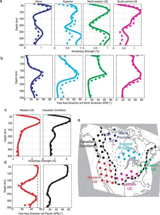
Average depth profiles of anisotropy strength (a and c) and fast axis direction (b and d) for six subregions of the North American continent, colour coded as shown in (e). Broken lines are the results of the inversion using only waveforms, and solid lines are those obtained when SKS splitting data are included. Note that the direction of anisotropy recovered is stable in both cases, whereas the anisotropy strength recovered is larger at depths greater than 200 km for the central parts of the continent, which helps to improve the fit to the observed SKS data. In (a) and (b) the anisotropy direction becomes subparallel to the North American APM below 200 km, with a maximum amplitude around 270 km. Noteworthy is the large anisotropy strength observed at 80–100 km depth in the western US (WUS) (c) and the Canadian Cordillera (d), which corresponds to sublithospheric depths. Between 100 and 150 km depth, the fast axis direction rotates from subparallel to the North American APM to a direction closer to the Pacific APM. Deeper in the western US the fast axis direction shows complexity due to the combined effects of the Pacific APM, current Juan de Fuca subduction, and possibly northeastern flow associated with the northward extension of the East Pacific Rise.

Open in new tabDownload slide

We have shown that large variations in azimuthal anisotropy exist both horizontally and vertically in the NA upper mantle. We have also shown that the strength of azimuthal anisotropy (G) presents maxima at and below the LAB in both the WUS and under the craton, where the fast axis direction is parallel to the APM. The maximum in G is much stronger in the WUS where it is shallow (∼70 km); while under the craton it is deeper than 250 km (Fig. 3). However, we also have seen from synthetic tests that the amplitude loss in G in the inversion is strong at depths greater than 250 km (Figs S1 and S10–S14). We therefore cannot assert quantitatively how much weaker the lithosphere–asthenosphere coupling is under the craton.

Another interesting question is what the relative contributions of the lithosphere and asthenosphere anisotropy are to the observed apparent SKS splitting. In Fig. 14(a), we compare the predictions of our complete model to the observed splitting; the fast axis directions match the measurements very well: 56 per cent for the overall variance reduction in SKS splitting, as defined in MR07_1, for the joint inversion, compared with 17 per cent for waveform only inversion (a 56 per cent variance reduction is large, considering the small scale lateral variations in splitting direction and strength that our long wavelength parametrization cannot account for). In particular, as discussed in YR10b, in the WUS, the depth integrated effects of our 3-D anisotropy model can explain the apparent circular pattern of SKS splitting measurements observed in Nevada without the need to invoke any local anomalous structures, as we discuss further below. Good matches are also seen in Alaska, the Slave craton, the western/central Superior, the Canadian Appalachians and the north-eastern US. Mismatches occur in a few places, mostly along the transition from the thick craton lithosphere to the thin WUS lithosphere: that is, the western Canadian Cordillera, the northeastern Colorado Plateau, and the southeastern US. In these regions the SKS data set also shows rapid spatial fast axis direction changes, which are beyond the horizontal resolution of our present azimuthal anisotropy model (∼500 km).

Figure 14

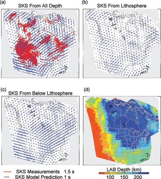
Apparent SKS predictions from various portions of the model space: (a) full depth of the inverted 3-D models; (b) lithospheric portion of the 3-D models assuming isotropic structure below, using the lithosphere thickness shown in (d); (c) deeper portion of the 3-D models assuming an isotropic lithosphere. Red bars in (a) are the SKS measurements for comparison. (d) is the estimated LAB map of the North American continent. Note LAB depths shown in (d) are based on vertical gradients in azimuthal anisotropy beneath the craton and the Phanerozoic eastern US, and on vertical gradients and peak values of radial anisotropy in the western US. If the latter definition was employed in the Phanerozoic eastern US, LAB depths would in general be shallower than those shown here.

Open in new tabDownload slide

Using the lithosphere–asthenosphere boundary (LAB) depth derived from our combined 3-D isotropic, radially and azimuthally anisotropic model, we compute separately contributions of the lithosphere and asthenosphere to the apparent SKS splitting parameters at the surface (Figs 14b and c). We focus more on the fast splitting axis direction, because of the uncertainty on the anisotropy G strength at large depths, thus the model predicted splitting times, which take the form of a sum of two depth integrated terms, respectively proportional to G_c and G_s, are not as well recovered as the model predicted fast axis direction.

Close examination shows that the model predicted fast axis directions are not necessarily entirely controlled by either the lithosphere or the asthenosphere (Figs 14b and c). Large contributions from the lithosphere are seen in the southern border of the Colorado Plateau in Arizona, New Mexico and neighbouring Mexican states; in Alaska; and in northeastern Canada. Large contributions from below the lithosphere are seen offshore Baja California, in southern and central California, western Superior, central, southeastern and northeastern US. In some areas the fast axis directions are similar in the lithosphere and asthenosphere, in which case they both contribute to the overall apparent SKS predictions. These regions include the Slave craton and the current Juan de Fuca subduction system (in Washington and Oregon; see also Fig. 8b).

The circular pattern of the SKS splitting noted in Nevada has been linked to a P-wave velocity anomaly, extending from depths shallower than 100 km into the transition zone (West et al. 2009). However, while this feature does appear in the P-wave model of Xue & Allen (2010), it is missing at ∼100 km depth in the P-wave models of Burdick et al. (2009) and Sigloch et al. (2008), the P- and S-wave models of Obrebski et al. (2010) and the S-wave model of Xue & Allen (2010). Instead high velocity starts at >200 km depth and extends into the transition zone (Sigloch et al. 2008; Burdick et al. 2009; Obrebski et al. 2010; Xue & Allen 2010). Our surface wave model shows this anomaly is deeper than 250 km and extends to the north at the top of the transition zone (Figs 4, 5 and 11). Our preferred interpretation is that it is part of the subducted Juan de Fuca slab. The circular pattern of the SKS splitting is well predicted by our azimuthal anisotropy model (Fig. 14), and is discussed in detail in YR10b.

Finally, we note that in this study, we have stopped short of considering the possibility of tilted axis of anisotropy, so that in some regions where such a tilt might be strong (e.g. Gaherty 2004; Plomerová & Babuska 2010), the azimuthal anisotropy strength may not reflect the true strength of anisotropy. There are regions where this is likely, in particular, in places where ξ < 1 (i.e. in the WUS asthenosphere as well as in some patches in the lower lithosphere under the craton).

5 Conclusions

The availability of high quality digital data, and in particular data from the EarthScope USArray TA deployment has allowed us to develop a radially and azimuthally anisotropic model of the NA upper mantle from the joint inversion of long period seismic waveforms and SKS splitting data. Combining the results of V_s, ξ and azimuthal anisotropy inversion brings out the spatial correspondence of some key features in upper-mantle structure:

• 1

  The contrast between the WUS and the craton in both isotropic and anisotropic structure, and the sharp transition between the two regions (Figs 4–7), closely following the RMF.

• 2

  The WUS is characterized by slow velocities and strong azimuthal anisotropy at shallow depths (<200 km), but weak anisotropy and faster than average velocities at depths greater than 250 km, while ξ < 1 at depths greater than 150 km.

• 3

  In contrast, in the craton, azimuthal anisotropy is weak at shallow depths, but stronger below the lithosphere, at ∼300 km, where it is likely to be even stronger in reality, given the poor recovery of amplitudes at those depths.

• 4

  The Colorado Plateau stands out as a tilted thick lithospheric block which separates upward flow from the south (East Pacific Rise) into an eastern branch, under the Rio Grande rift, and a western branch, into the Basin and Range.

• 5

  In the asthenosphere, the fast axis direction of the azimuthal anisotropy beneath the craton agrees with the absolute plate motion direction in a fixed hotspot reference frame (model HS3-NUVEL 1A) better than with the no-net rotation model (NNR-NUVEL 1A), especially in the centre and east of the NA craton. In the tectonically active WUS and Canadian Cordillera, both reference models indicate very similar directions, which agree with the fast axis direction in our model at asthenospheric depths.

• 6

  The combination of maps in V_s, ξ and azimuthal anisotropy reflect contrasts in structure between the lithosphere and asthenosphere across the continent, and the considerable variations in LAB depth, which range from less than 80 km in the WUS to over 200 km in the craton, with a sharp lateral gradient along the RMF.

• 7

  Directions of azimuthal anisotropy vary with depth in the lithosphere, but align with the absolute plate motion in the asthenosphere. The alignment of the fast axis of anisotropy with the NA APM between 70 and 100 km depth throughout the WUS indicates that, to first order, the uppermost part of the mantle is moving along with the NA Plate and is not strongly coupled to deeper mantle flow, providing some constraints on geodynamical modelling (e.g. Silver & Holt 2002; Becker et al. 2006).

• 8

  We suggest the presence of small scale convection with a wavelength of 1500–2000 km below the lithosphere under the craton. This pattern extends into the WUS, where the pattern of anisotropy below 150 km is dominated by mantle dynamics and related to subduction and spreading associated with the EPR and its continuation under the continent.

Acknowledgments

This study was supported by NSF EAR-0643060 grant to BR and EAR-0641772 to KF. We thank the IRIS DMC and the Geological Survey of Canada for providing the waveforms. We are grateful to K. Liu, M. Fouch, R. Allen, A. Frederiksen, A. Courtier, G. Soto and I. Bastow for sharing their SKS splitting measurements and S. Whitmeyer and K. Karlstrom for providing their Proterozoic Laurentia structural map. Comments from two anonymous reviewers greatly improved the manuscript. This is BSL contribution 10–12.

Supporting Information

Additional Supporting Information may be found in the online version of this article:

Resolution tests, LAB picking in the WUS and Smoothed SKS dataset.

Please note: Wiley-Blackwell are not responsible for the content or functionality of any supporting materials supplied by the authors. Any queries (other than missing material) should be directed to the corresponding author for the article.

References