Ground deformation in an area later damaged by an earthquake: Monitoring the Avcilar district of Istanbul, Turkey, by satellite radar interferometry 1992–1999

Summary

Introduction

Avcilar is a small city of over 200 000 inhabitants, located at 25 km west of Istanbul (Fig. 1). The urbanized centre of Avcilar is situated east of Kucukcekmece Lake, a lagoon connected to the Marmara Sea. The main residential area of Avcilar is on a NW-SE elongated hill that rises to 135 m elevation. With an annual population growth rate of 6 per cent per year between 1990 and 2000, it is one of the fastest-developing areas of Istanbul (TUIK 2000). Accordingly, it makes sense to analyse the risks posed by the natural hazards in the region.

Figure 1.

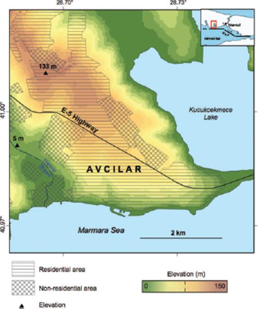
Map of the Avcilar district of the Istanbul metropolis, showing topographic elevation (colours), residential areas (parallel hachure), non-residential areas (crossed hachure) and the E-5 highway (black line). Most of the buildings damaged in the 1999 earthquake are located between the highway and the coastline (Tezcan et al. 2002). Inset shows the trace of the North Anatolian Fault (NAF) and the outline of the study area (small rectangle).

Open in new tabDownload slide

Avcilar county was severely affected by the M 7.4 Izmit (Kocaeli) earthquake of 1999. At least 273 people were killed and 1450 buildings damaged there, as a result of the earthquake (Tezcan et al. 2002). Some 11 per cent of the buildings were destroyed or damaged beyond repair (Tezcan et al. 2002). The damage in Avcilar County was much greater than in the whole metropolitan of Istanbul. Since Avcilar is located over 120 km from the epicentre of the earthquake, the severe damage must have been caused by amplified shaking (Tezcan et al. 2002; Ergin et al. 2004). The maximum ground acceleration recorded on soft sediment near Avcilar was 0.25g, more than six times higher than the acceleration recorded on bedrock in Istanbul during this earthquake (Tezcan et al. 2002). Such shaking occurs when soft soil or rock overlying hard bedrock amplify seismic waves (Field et al. 2001). At Avcilar, ‘trapping’ of body waves and subsequent resonance was the primary cause of the site amplification (Ergin et al. 2004). Beyond the site amplification, improper building practices, such as using sea sand to make concrete, also contributed to the damage (Cagatay 2005).

The Avcilar area is located within a few tens of kilometers of the North Anatolian fault, which splits into several splays where it enters the Marmara Sea (Armijo et al. 2002; Polonia et al. 2002; Le Pichon et al. 2003). Although interseismic strain accumulates on the North Anatolian fault at a rate of the order of ∼10⁻⁷ yr⁻¹ (Reilinger et al. 2006), this predominantly horizontal signal will not contribute more than 1 mm yr⁻¹ to the fringe patterns in the interferograms considered here, because the study area spans less than 5 km in the N-S direction perpendicular to the strike of the fault.

The Avcilar area has been severely affected by landslides for many years (Ormeci 1972; Duman et al. 2005a,b; Duman et al. 2004; Alparslan et al. 2006). Landslides around Avcilar tend to occur in lithologies composed of permeable sandstone layers and impermeable claystone, siltstone or mudstone layers (Ormeci 1972; Duman et al. 2004). In particular, the Cukurcesme sandstone and Gurpinar clay formations are very weak, with unconfined compressive strengths as low as 200 kPa (Tezcan et al. 2002). The landslides occur preferentially during the wet season, as water enters the permeable upper soil layers and weakens them. The bedding of the upper layers of sediment dips approximately 10° towards the southwest. In addition, landslides also occur on oversteepened slopes near the shorelines, for example, near Ambarli, where buildings have been evacuated (ELC 2005). Although landslides have been known to occur for years, quantitative studies are still in their early stages. In the southwest corner of the study area, Kalkan et al. (2003) found a displacement of 30 cm vertically and 130 cm horizontally between 1999 and 2003 by comparing traditional, levelling and GPS surveys.

In addition to coseismic shaking and landslide activity, liquefaction is also a concern in Avcilar. Although no evidence of coseismic liquefaction was observed around Avcilar immediately following the 1999 earthquakes, the sediments would be susceptible to liquefaction in the event of a large earthquake located closer to Avcilar (Tezcan et al. 2002). The shallow sedimentary layers are saturated or partly saturated with water, especially in the urban part of Avcilar, where the depth to ground water varies between 6 and 16 m (Tezcan et al. 2002). There, the water level in a well can change as much 80 cm in a month (ELC 2005).

In this paper, we analyse synthetic aperture radar (SAR) images acquired by the ERS-1 and ERS-2 satellites between 1992 and 1999 to measure deformation in and around Avcilar.

Methods

Interferometric analysis of SAR images (InSAR) is a geodetic technique that calculates the interference pattern caused by the difference in phase between images acquired by a SAR sensor at two distinct times. The resulting interferogram is a contour map of the change in distance between the ground and the radar instrument. These maps provide a spatial sampling density of at least ∼100 pixels km⁻², a precision of ∼10 mm and an observation cadence of ∼1 pass month⁻¹. This remote-sensing tool has been demonstrated and validated for many actively deforming areas, including natural earthquakes and anthropogenic activity, as reviewed by Massonnet & Feigl (1998).

Data selection and interferometric analysis

We have analysed 47 SAR images acquired by the ERS-1 and ERS-2 satellites in frame 2783 of track 338 on different dates (epochs) between 1992 and 2002, as described in detail by Akarvardar (2007). Beginning with raw data, we follow the standard procedure for two-pass interferometry (e.g. Massonnet & Feigl 1998) using version 4.1 of the PRISME/DIAPASON software developed at the French space agency (Massonnet et al. 1994; CNES 1998, 2006). The details of this procedure are described elsewhere (Pedersen et al. 2003; Akarvardar 2007). The orbital trajectories have been estimated with decimetre accuracy (Scharroo & Visser 1998). The digital elevation model has a posting of 40 m and a vertical accuracy of ∼5 m (IMM & JICA 2002). We apply power-spectral filtering to all the interferograms (Goldstein & Werner 1998).

To select the data set, we proceed in several steps. First, we retain only those interferometric pairs that have an ambiguity height greater than 100 m in absolute value and a difference in azimuthal Doppler frequency Δf_D less than 0.4 times the pulse repetition frequency (PRF) in absolute value. Since all of the interferometric pairs analysed here have an ambiguity height h_a, as defined by Massonnet & Rabaute (1993), greater than 100 m in absolute value, we expect topographic errors to contribute less than 1/10 of a cycle, or 3 mm, to the uncertainty of the range change measurement. After applying these two threshold operations, we eliminate pairs that show poor interferometric correlation around Avcilar, retaining 36 pairs that include 28 epochs. Of these, we retain the 19 epochs before the Izmit earthquake on 1999 August 17.

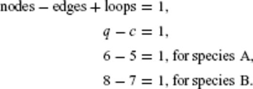
Next, we consider the 19 selected epochs in terms of ‘species’. As defined by Feigl & Thurber (2009), a species is the set of single-epoch images that can be combined pairwise to form useful interferometric pairs. According to this definition, any epoch belonging to a given species can form a useful interferometric pair with any other epoch belonging to the same species, either by direct calculation or by construction, that is, linear combination of pairs of other members of the species. Some images do not form useful interferometric pairs because of temporal decorrelation, orbital separation (as measured by the ambiguity height) or differences in azimuthal Doppler frequency. For example, we were unable to find any useful interferometric pairs spanning time intervals longer than 3 yr. The 19 epochs yield 33 useful pairs that form a single large species.

In this species, some of the epochs form only one or two pairs. By eliminating such ‘isolated’ epochs (orbits −11002, −23370 and −21366), we reduce the data set by three epochs. Two other epochs are excluded because they form only poor pairs. For example, the pairs including epoch 1998.98 (orbit + 19928) are eliminated because of temporal de-correlation. When combined with epoch 1995.72 (orbit −21867) and 1993.07 (orbit + 7996), this epoch yields pairs spanning over 3 yr that do not show coherent fringe patterns. Epoch 1996.58 (orbit + 6703) appears to have atmospheric variations because all the pairs including it show characteristic, crenulated fringes (e.g. Massonnet & Feigl 1995).

After eliminating three isolated epochs and two epochs that form poor pairs, we retain the 14 epochs listed in Table 1, for further analysis. Pairwise combination of these 14 epochs gives the 12 pairs listed in Table 2. This list forms two species. The first species includes six epochs (labelled A in Table 1) that form five pairs (drawn as red line segments in Fig. 2). The second species includes eight epochs (labelled B in Table 1) that form seven pairs (drawn as blue line segments in Fig. 2). In Fig. 2, the line segments represent pairs connecting epochs, forming an incidence graph (Strang & Borre 1997). Since neither of the paths connecting all the epochs within each species forms a closed loop, we see that the data set does not include any redundant pairs. Mathematically, the two incidence graphs reduce to trees, according to a formula attributed to Euler (Strang & Borre 1997):

1

Table 1.

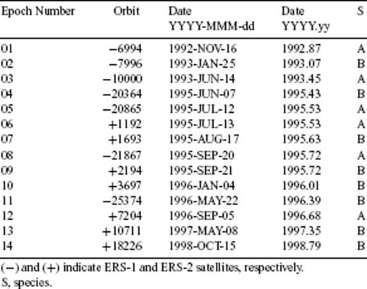
Acquisition epochs for ERS SAR images included in inversion.

Open in new tabDownload slide

Table 2.

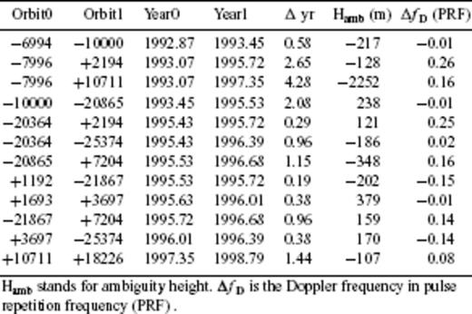
Interferometric pairs included in inversion.

Open in new tabDownload slide

Figure 2.

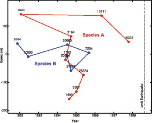
Orbital separation versus time for the radar images analysed in this study, showing the 14 individual images (epochs) as points. The interferometric pairs considered here are shown as line segments connecting the points. The pairs fall into two distinct species, labelled A (blue) and B (red). The horizontal coordinate displays the acquisition date (epoch) of each image in decimal years. The vertical coordinate shows the orbital separation or perpendicular component of the ‘baseline’ vector between the positions of the radar sensor at the acquisition epoch. For a single image, the orbital separation is calculated with respect to a virtual centroid trajectory. The dashed line shows the date of the M 7.4 1999 August 17 Izmit earthquake.

Open in new tabDownload slide

The interferograms corresponding to the 5 + 7 = 12 pairs constitute the data set considered in the modelling described below.

To reduce the volume of the data set for inversion, we consider various methods for identifying and selecting the most reliable pixels. Following previous work, we evaluate two criteria: one based on the spatial coherence of the phase measurements and the other based on the temporal scatter of the amplitude measurements (Ferretti et al. 2000; 2001; Lyons et al. 2002; Colesanti et al. 2003). For this part of the analysis, we use all 47 amplitude images acquired between 1992 and 2002 to calculate the ‘amplitude dispersion index’D_A, as defined by Ferretti et al. (2000, 2001). To apply the second criterion, Akarvardar (2007) considers a set of 15 pairs to calculate a ‘multiple coherence’γ, as defined by Colesanti et al. (2003). The pixels retained for the estimation procedure have an amplitude dispersion index D_A less than 0.25 and a multiple coherence γ greater than 0.5 in absolute value. Applying both criteria, we retain 163 pixels in the area of interest for the inverse modelling. Their areal density is ∼3 pixels km⁻². Applying only the coherence threshold, we obtain 387 pixels with a density of ∼7 pixels km⁻². Since the modelling results improve slightly when using the points selected with the coherence threshold alone, we retain the 387 pixels so selected, for the subsequent analysis.

Modelling

Feigl & Thurber (2009) have developed a scheme, called General Inversion for Phase Technique (GIPhT), for analysing interferograms without unwrapping them. GIPhT defines a misfit cost function in terms of wrapped phase. It may be interpreted geometrically as the L₁ norm of the angular deviations between the observed and modelled values of the phase change. It is equivalent to the circular mean deviation (Mardia 1972) of the wrapped phase residuals if their mean direction is negligible. By minimizing the cost with a simulated annealing algorithm (Kirkpatrick et al. 1983), this approach can solve simultaneously for both linear and non-linear parameters.

For a single pixel in an interferometric pair, we write the phase change between the first (master) image acquired at time epoch t₁ and a second (slave) image acquired at epoch t₂ as

2

Generalizing to a time-series of images, with q ≥ 2 epochs forming c ≥ 1 pairwise combinations, we write the vector of phase changes for the kth pixel as the product of a matrix and a column vector:

3

where D^(k)_ij is a differencing matrix defined so that its element at row i and column j equals −1 when epoch t_j is master, +1 when epoch t_j is slave and 0 elsewhere. The row index i ranges over the c pairs and the column index j ranges over the q epochs. Thus, the differencing matrix D^(k)_ij for pixel k has c = 12 rows and q = 14 columns. It has a rank deficiency of 2 because it describes two species (Feigl & Thurber 2009).

The system of equations described by (2), thus, specifies the phase change at location (pixel) k in the interferometric pair spanning the ith time interval. As written (2), the phase change is a function of time (indices i and j range over epochs) and position (index k ranges over pixels). The order of the pixels assigned by the index k is arbitrary. In other words, we do not assume any particular spatial structure for the 2-D arrays of pixels. For simplicity, however, we will assume that the positional dependence and temporal dependence are ‘separable’, as suggested by Fialko (2004). Accordingly, we write the modelled phase value for a single pixel with index k at a single epoch t_i as

4

where f is a function of time only (∂f/∂x = 0), g is a mapping function of position only (∂g/∂t = 0), which describes the signal of interest, the geophysical deformation on the ground, and each h_i is a mapping function of position only (∂h/∂t = 0), which describes the nuisance effects pertaining to a single epoch such as tropospheric perturbations or errors in the satellite's orbital trajectory. The modelled value of the change in phase for a single pixel with index k over the time interval from t_i to t_j is

5

where the scalar function f(t) describes the time dependence of the geophysical deformation whereas the mapping function g^(k) = g(X^(k)) describes the spatial dependence as a function of the position coordinate of the kth pixel , written as easting, northing and upward components reckoned in a local Cartesian reference system.

For Avcilar, we assume secular deformation with constant rate so that f (t) = t-t₁, where t₁ is the first epoch expressed in years. The shape of the deformation field in map view is . In this equation, u is the vector field of annual displacements at the surface of the Earth, calculated using Mogi's (1958) formulation for a infinitesimal spherical source buried in an elastic half-space. The term is a position-dependent unit vector, pointing from the pixel on the ground to the radar sensor along the line of sight. The set of model parameters m of interest are thus the parameters describing the three position coordinates of the source (easting, northing and depth), as well as its change in volume ΔV. For Avcilar, we describe the source as three deflating Mogi sinks. Their depths and volume changes are equal. Their relative horizontal positions are fixed, such that the easting coordinates of the second and third sources are 1800 and 1550 m less than the first one's, respectively; their northing coordinates are 500 and 3300 m greater than the first one's, respectively.

Each of the nuisance functions h_i^(k) depend on position (pixel index k). There is one such function for each time epoch t_i. One simple parametrization is to consider a linear function of elevation at each epoch t_i:

6

where summation over the pixel index k is not implied. This expression accounts for the effect of the atmosphere. The vertical component h_U of the phase gradient accounts for the change in refractive index of the atmosphere with elevation. Its value can be as large as , or approximately one C-band fringe per kilometre of topgraphic relief (e.g. Hanssen 2001). The term h₀(t_i) is an additional phase offset that accounts for the tropospheric delay averaged over all pixels observed at the time epoch t_i. In other words, the model accounts for tropospheric fringes that look like a scaled version of the topographic relief. We estimate one gradient parameter and one offset parameter for each of the 14 epochs. By neglecting horizontal phase gradients, we are neglecting orbital effects, a reasonable approximation over the small (∼4 km) dimension of the study area.

The inverse problem consists of estimating the model parameters m from the phase data . Using GIPhT (Feigl & Thurber 2009), we solve the inverse problem using a simulated annealing algorithm (Kirkpatrick et al. 1983), as implemented by Cervelli et al. (2001). This approach begins with an initial estimate of the model parameters. To further constrain the inversion, we can place upper and lower bounds on each parameter.

For the source parameters, we set the bounds on the depth and annual volume change rate to within ±30 per cent of the initial values. For the easting and the northing coordinates of the source, the bounds are set to within ±600 m of the initial location.

Initially, we set the initial values of the tropospheric parameters to 0.03 ×10⁻³ at each of the 14 epochs. This value represents the worst case (e.g. Hanssen 2001). It corresponds to a difference in path delay of 4 mm in range between a pixel located at the highest point in the Avcilar area at an elevation of 135 m and a pixel located at sea level. Although the epochs with atmospheric artefacts can be recognized by pairwise logic, it is not easy to decide the sign and the magnitude of the atmospheric phase contribution in the interferograms. Running the GIPhT on trial-and-error basis, we find new values for the tropospheric parameters, as listed in the second column of Table 3. These values then form the initial estimates in our preferred solutions. The upper and lower bounds for the 14 tropospheric gradient parameters h_U(t_i) are set to within ± 0.056 × 10⁻³ of the initial estimates. Similarly, the upper and lower bounds for the 14 additive offset parameters h₀(t_i) are set to ± 14 mm.

Table 3.

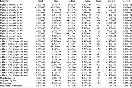
Estimated parameters.

Open in new tabDownload slide

Once the simulated annealing algorithm has located the minimal cost, we retain the corresponding values of the parameters as the final estimate of the model parameters, as listed in the third column of Table 3. To evaluate the uncertainty of these estimates, we consider each parameter separately to calculate cost as a function of the parameter's value. The minimum of this function corresponds to the final estimate of this parameter, as expected. The half-width of this function at a cost corresponding to 69 per cent confidence gives the 1-sigma uncertainty (standard error) of the corresponding parameter estimate (Press et al. 1992).

Results

Most of the interferograms show fringes shaped like a rounded triangle centred on the urbanized part of Avcilar. For example, Fig. 3 shows two interferograms and illustrates how the GIPhT approach can distinguish the subsidence signal from the atmospheric nuisance. Since the interferogram for the pair combining epochs 1996.01 and 1996.39 shown in Fig. 3(a) spans a time interval of only 0.38 yr, the expected shift from secular subsidence is unlikely to exceed 2 mm in range or 0.1 cycle in phase (One cycle of colour composing a single fringe represents 28 mm of range change for all the ERS interferograms shown here). Since the observed fringes range from yellow in the centre of the triangle to red at its edges, for a differential phase shift of 0.3 cycles, we conclude that the tropospheric contribution is large. Indeed, the additive offsets estimated by the GIPhT procedure are 2.9 ± 3.1 and 6.4 ± 2.6 mm for the master (1996.01) and slave (1996.39) epochs, respectively. For the same epochs, the estimates of the vertical phase gradient are −0.03 ± 0.04 × 10⁻³ and 0.003 ± 0.03 × 10⁻³, respectively. In contrast, the interferogram shown in Fig. 3(b) shows an increase of approximately 0.8 cycles between the edge of the triangle (red) and its centre (yellow). If interpreted as subsidence alone, this value would imply as much as 12 mm yr⁻¹ of range increase when averaged over the 2.08 yr time interval. Yet, the tropospheric contribution in Fig. 3(b) is of the same order of magnitude as that in Fig. 3(a). The estimated values of the additive offsets are −1.3 ± 3.4 and −4.6 ± 3.6 mm for the master (1993.45) and slave (1995.53) epochs, respectively (Table 3). The estimated values of the vertical gradients are −0.02 ± 0.04 and −0.06 ± 0.04 × 10⁻³, respectively. These values imply that tropospheric effects contribute as much as 0.22 cycle of phase to the interferometric fringe pattern. Accounting for them reduces the maximum rate of range change by approximately 2.9 mm yr⁻¹, again averaged over 2.08 yr.

Figure 3.

Examples of observed interferograms spanning (left-hand panel) the time interval between epoch 1993.45 (orbit −10000) and epoch 1995.53 (orbit −20865) and (right-hand panel) the time interval between epoch 1992.87 (orbit −6994) and epoch 1995.53 (orbit −20865). Coordinates are north latitude and east longitude in decimal degrees.

Open in new tabDownload slide

Fig. 4 shows the interferogram spanning 1.44 yr between 1997.35 and 1998.79. Fig. 4(a) shows the observed interferogram with a similarly shaped, rounded triangular fringe pattern. The colours running from orange at the northwest corner of the rounded triangular shape to blue at its centre indicated approximately 0.5 cycles of range increase, corresponding to motion away from the satellite. Assuming the Mogi (1958) formalism and three sources, we begin with a initial estimate of the model parameters based on a trial-and-error approach (Akarvardar 2007). Using them in the forward calculation produces the pre-fit residual fringe patterns shown in Fig. 4(c).

Figure 4.

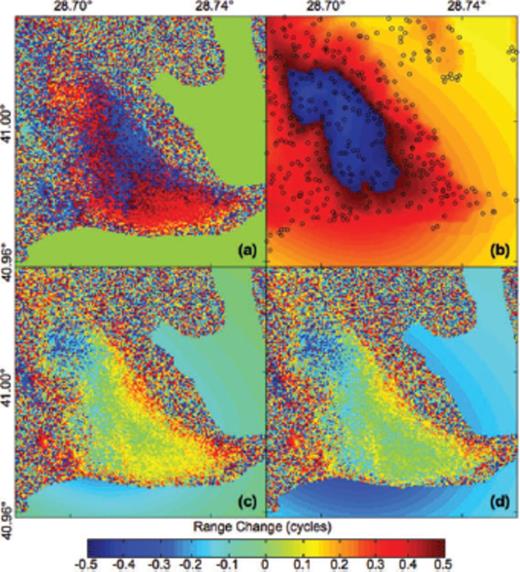
Interferograms for the pair spanning the time interval between 1997.35 (orbit +10711), and 1998.79 (orbit +18226). The panels show: (a) observed fringe pattern. (b) Simulated fringes calculated from the final estimate of model parameters. The dots are PS pixels used for calculating the final estimates. (c) Wrapped residual fringes formed by subtracting the simulated fringes calculated from the initial estimate of the model parameters from the observed fringe pattern. (d) Wrapped residual fringes formed by subtracting the simulated fringes calculated from the final estimate of the model parameters from the observed fringe pattern. Note that the final residuals in the middle of the rounded triangle have a range of ±0.1 cycles for the time interval of 1.44 yr. One coloured fringe corresponds to one cycle of phase change or 28 mm of range change.

Open in new tabDownload slide

To optimize the fit of the simulated fringe pattern to the observed one, we apply the methods described in the previous section to the set of 12 interferometric pairs listed in Table 2. The final estimate for the depth of the three Mogi sinks is 2.4 ± 0.4 km. Their total volume is decreasing at a rate of (8 ± 2) × 10⁴m³ yr⁻¹. These values produce the maximum rate of vertical subsidence of 6 mm yr⁻¹ at a location in the centre of the wedge. This estimate of the parameter set produces the simulated fringe patterns shown in Fig. 4(b). The corresponding post-fit residual interferogram (Fig. 4d) shows less unmodelled signal than the pre-fit residual interferogram (Fig. 4c). The map of the marginal costs for the final estimate (Fig. 5b) shows lower values than for the initial estimates (Fig. 5a).

Figure 5.

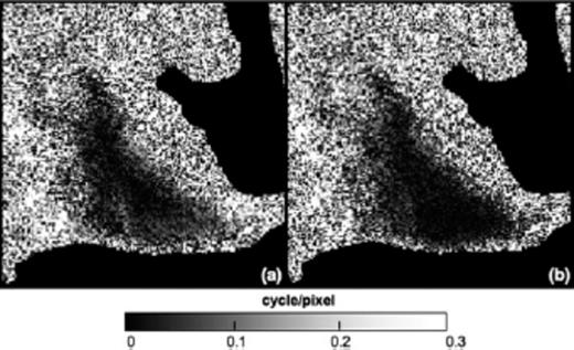
Maps of the angular deviations contributed by individual pixels in the interferometric pair spanning the time interval 1997.35–1998.79 calculated from two sets of model parameters: (a) initial estimate and (b) final estimate. The scale ranges from an angular deviation of cycle (dark shading) to 0.5 cycle (light shading).

Open in new tabDownload slide

In addition to the subsidence signal, the interferometric pair shown in Fig. 4 also shows tropospheric noise. The additive offsets are 11 ± 3 mm and 14 ± 5 mm for the master epoch 1997.35 (orbit +10711) and the slave epoch 1998.79 (orbit +18226), respectively. These values are among the largest (in absolute value) of any of those estimated here (Table 3).

Fig. 6 shows the observed and modelled values of range change in a profile running from west to east through Avcilar. The modelled curve computed from the final estimates fits the data points within 0.2 cycles in most places. The final estimate of the model parameters fits the set of 12 observed interferograms better than the initial estimate. The cost values for the null, initial and final estimates are 0.261, 0.213 and 0.184 cycle per datum, respectively, for the 12 × 387 = 4644 phase measurements included in the inversion. Both the initial and final estimates of the 32 free parameters fit the data significantly better than does setting all parameters to zero. In addition, the final estimate of the model parameters fits the data significantly better than does the initial estimate. To make these inferences, we assume that the phase residuals are compatible with a von Mises distribution, as suggested by the histograms shown in Fig. 7. Then we perform a two-sample test to test the null hypothesis that the concentration parameters of two sets of residuals are equal by calculating the test statistic in eq. (7.3.23) of Mardia & Jupp (2000, p. 133), as described by Feigl & Thurber (2009).

Figure 6.

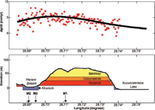
Profile on an east-west line at latitude N40.98° showing (above) the observed (circles) and modelled (thick curve) rates of range change and (below) the topographic elevation (thin curve) with a vertical exaggeration of 10: 1, as well as a schematic cross-section sketched from the geologic map in Fig. 1. The contacts between the rock formations are assumed to be horizontal.

Open in new tabDownload slide

Figure 7.

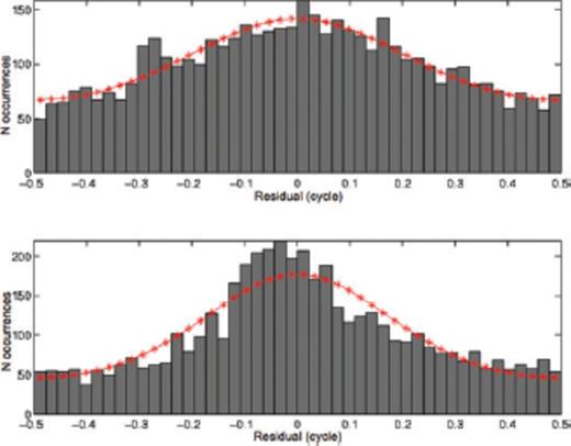
Histogram of the wrapped phase residuals in cycles for the initial estimate (above) and final estimate (below). The curves indicate the numbers of occurrences expected from von Mises distributions with a mean direction , sample size n = 4644 and concentration parameter , for the initial residuals, and , for the final residuals.

Open in new tabDownload slide

To verify the robustness of the estimates of the model parameters, Akarvardar (2007) has performed the GIPhT analysis on a slightly different data set. Changing the criteria to select pixels with amplitude dispersion index D < 0.25 and coherence ǀγǀ > 0.5 reduces the number of pixels included in the inversion to 163. The resulting estimates of the depth and rate of volume change for the source are only marginally different from those listed in Table 3. Accordingly, we infer that the estimation procedure is robust to the choice of pixels and interpret the estimates listed in Table 3 below.

The estimates of the additive offset and vertical fringe gradient parameters suggest that the troposphere contributes to the range change in a manner that varies considerably in time. For example, 6 of the 14 epochs have additive offset values h₀(t_i) estimated to be greater than 10 mm. Similarly, the vertical gradient reaches a value of , equivalent to 12 ± 7 mm of range over 130 m of topographic relief in the worst case (epoch 1998.79). Similarly, large values occur at several other epochs, as listed in Table 3. These values approach the worst-case values documented elsewhere (Goldstein 1995; Massonnet & Feigl 1995; Zebker et al. 1997; Williams et al. 1998; Beauducel et al. 2000; Hanssen 2001). Since the tropospheric effects do not depend on the time interval Δt = t_j-t_i between the two epochs, our approach, using GIPhT, can separate them from the subsidence signal, which does depend on the time interval Δt (Feigl & Thurber 2009). Accounting for the tropospheric effects allows us to map the average rate of vertical subsidence in Fig. 8.

Open in new tabDownload slide

Open in new tabDownload slide

Figure 8.

Map of mean annual rate of range change in the observed (a), modelled (b) and final residual (c, next page) fields. The observed values have been unwrapped using the final model. They have also been corrected for tropospheric effects by subtracting the value of the nuisance functions calculated with the final estimate of the tropospheric parameters. Contours are in mm yr⁻¹. Downward subsidence appears as a positive rate of range change.

Discussion

To increase confidence in the InSAR results, we compare them to other observations of ground deformation around Avcilar. The crescent-shape pattern of subsidence rate resembles the one produced by GMES Terrafirma (Aktar & Browitt 2006), using a data set that partially intersects ours but a different analysis strategy (e.g. Ferretti et al. 2001). Although both approaches assume a constant rate of subsidence, our approach estimates the parameters in a simple geophysical model. Repeated levelling surveys near harbor in the SW corner of study area (P1 and P2 in Fig. 9) indicate 11–12 mm of vertical subsidence over 30 months (Kalkan et al. 2003), or an average rate of 4 to 5 mm yr⁻¹, in good agreement with the 3–4 mm yr⁻¹ of vertical motion we find in this location using InSAR (Fig. 8a). A GPS station (P3 in Fig. 9) installed in the east half of the study area following the 1999 earthquakes, indicates an average downward displacement rate of 12 ± 2 mm yr⁻¹ (Ergintav et al. 2007). This value is more than twice the 5 mm yr⁻¹ rate we find in this location with InSAR during the time interval 1992–1999 (Fig. 8a).

Figure 9.

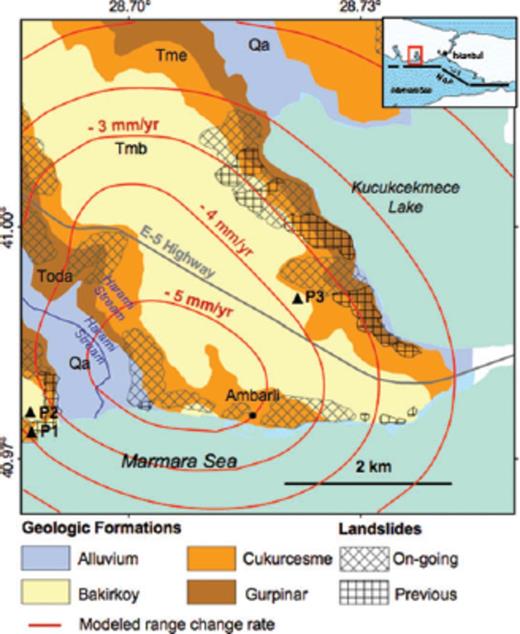
Interpretive map of the Avcilar district, showing four geologic units (colours) (Duman et al. 2004; Alparslan et al. 2006), rates of range change rate as in Fig. 8 (contours with values in mm yr⁻¹), locations of ongoing (cross-hachure) and previous (simple hachure) landslides (Duman et al. 2004; Alparslan et al. 2006).

Open in new tabDownload slide

In Fig. 8a, we plot the contours of the vertical velocity field measured by InSAR from Fig. 7(a) on a simplified geologic map. The rounded triangular shape of the rapidly (> 5 mm/yr) subsiding area resembles the pattern of alluvium and sediments in the Cukurcesme and Gurpinar formations. These sediments are unconsolidated, porous, permeable, saturated, and weak, as described in the introduction. They are susceptible to seismic amplification during earthquakes and landslides during rainfall. It seems possible that they may also have undergone compaction during the 1992–1999 time interval, causing at least part of the subsidence observed in the InSAR results. The geometric distribution of the volume decrease is certainly more complicated than the three infinitesimal (point) Mogi sinks assumed in our modelling. Accordingly, the final estimate of the Mogi depth may be too deep. In this case, the estimated reduction in volume may be too large because of the trade-off between these two parameters. Furthermore, the value of Poisson's ratio in the unconsolidated sediments (Ergin et al. 2004) is likely to be less than the value of 0.25 assumed in our modelling, possibly biasing the depth estimates (e.g. Cattin et al. 1999).

Although the constant-rate, three-sink Mogi model explains the first-order features of the interferometric data set well, some second-order features remain to be explained. For example, near (N40.97°, E28.74°) in Fig. 3(b), we see a transition in the fringe pattern between red and light blue, indicating an increase in range of 0.6 cycles in 2.08 yr. Assuming purely vertical motion at a constant rate, we find approximately 9 mm yr⁻¹ of subsidence, a rate that is faster than the value calculated from the model at that location. In this area, an active landslide may have deformed the ground surface in a manner that is more complicated than assumed in our separable model. Indeed, the anomalously high rate occurs near the coastal town of Ambarli, an area with a history of landslides. Similarly, the yellowish residuals on the west side of Fig. 8(c) show that the downward vertical displacement rate is 2–3 mm yr⁻¹ faster than that calculated from the model. This area, around Harami stream, has experienced landslide activity in the past; none has been reported during the 1992–1999 time interval (Duman et al. 2004). It may be that material transported in previous landslides may have continued to settle during the time interval spanned by the InSAR data set. Again, the motion of landslides at the surface is poorly described by our simple model for volume change at depth. Furthermore, if several different landslides deform more rapidly during the wet season than during the dry season, then the spatio-temporal pattern of the deformation would be more complex than the secular, separable field assumed here. Such a complex pattern would be difficult to constrain with the InSAR data set because most of the epochs that form good interferometric pairs are in the dry season. The issue of temporal decorrelation in the InSAR data may also complicate the interpretation of second-order features in the residual vertical velocity field shown in Fig. 8(c). Pixels on the surface of a muddy landslide deforming rapidly in the wet season are not likely to meet the criteria used to select data for the inversion. Since it selects only pixels with stable dielectric properties, the method may underestimate the rate of deformation.

Using InSAR to monitor the Avcilar area from 1992 to 1999 reveals ground deformation in the location that was later damaged by the M 7.4 Izmit (Kocaeli) earthquake of 1999. The association of ground deformation with earthquake damage may be interpreted in terms of weak, compressible material in shallow subsurface layers. Such material, described in detail in Section 1, is susceptible to seismic amplification during earthquakes and landslides during rainfall, as discussed above. Such an association of damage and weak material has been observed in other earthquakes. The M 8 Michoan event of 1985 shook the lake-bed sediments underlying Mexico City (e.g. Iida 1999). The M 6 Kozani-Grevena earthquake of 1995 damaged relatively recent buildings in areas with ‘siltey and clayey soils’ in Greece (Christaras et al. 1998). The M 6 Bay of Plenty earthquake sequence of 1987 produced maximal shaking (Modified Mercali Intensity IX) in areas of ‘soft, saturated sediments’ underlying the Rangitaiki Plains in New Zealand (Franks et al. 1989). The M 6 Northridge earthquake of 1994 induced settlement and liquefaction in soft ‘fill’ in California (Holzer 1994; Bishop & Day 1995; Field et al. 1997; Holzer et al. 1999). Ground failure in the New Madrid Seismic Zone has been attributed to ‘the development of a water-rich zone below the clayey surficial deposits’ (Tuttle & Barstow 1996). This region was also ‘subjected to repeated episodes of wide-scale liquefaction, ground subsidence and uplift’ (Doyle & Rogers 2005). The M 7.3 Izmit (Kocaeli) earthquake of 1999 also caused ground failure at Degirmendere, which caused a submarine slump and a tsunami (Tinti et al. 2006). The causative submarine landslide there was ‘mainly because of earthquake shaking rather than liquefaction’ (Aydan et al. 2008). In light of the observed association between weak subsurface material (as inferred from permanent deformation) and susceptibility to site (amplification) effects during earthquake shaking (as inferred from damaged buildings), a causal mechanism has been proposed. Indeed, ‘ground subsidence of the soft clay deposits might heavily influence S-wave propagation‘ (Iida 1999).

Conclusion

The InSAR results around Avcilar show increases in range that we interpret as downward motion at vertical rates as fast as 6 mm yr⁻¹. A simple four-parameter model consisting of three infinitesimal spherical Mogi sinks at a depth of 2.4 ± 0.4 km deflating at 78 000 ± 16 000 cubic metres per year fits the data with a cost of 0.1844 cycle per datum, for the 4644 phase measurements included in the inversion. The modelling also accounts for tropospheric effects. By parametrizing the deformation signal as a separable field, the GIPhT inversion scheme can distinguish it from the tropospheric noise, because the latter does not depend on time. The fit between the model and the InSAR data is significantly better than both the null hypothesis and the initial model with 95 per cent confidence, for 32 free parameters. The map of range residuals averaged over time shows some signatures that are not explained by the separable model. These unmodelled signatures may be related to the transient deformation of landslides that occurs locally in space and seasonally in time. The spatial distribution of the deformation signal resembles that of a shallow layer of unconsolidated, partially saturated soil (Cukercesme formation) with a relatively weak lithology. This layer appears to deform easily in several processes, including subsidence, landslide failure and seismic wave amplification. It may also be susceptible to failure induced by liquefaction during a large earthquake. Accordingly, it seems prudent to continue monitoring ground deformation by InSAR, especially in heavily populated areas such as Istanbul that are exposed to earthquakes.

Acknowledgments

We thank Ramon Hanssen for identifying the travelling salesman. We thank Cliff Thurber, Mustafa Aktar, Tuncer Edil and Herb Wang for interesting discussions. Two anonymous reviewers improved the clarity of the manuscript. All SAR data were provided by the European Space Agency, which holds the copyright to them under the terms and conditions of a Category-I project (number 3245) accorded to the authors. This work was partially supported by grants from the European Union (FORESIGHT 511139) and the French government ‘Agence National de Recherche’ (HYDRO-SEISMO).

References