


Summary
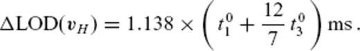
A number of core surface flow models have been inferred from geomagnetic field models by applying the frozen-flux induction equation. It is well known, however, that the flow is not fully resolvable. Because of theoretical and observational setbacks, the model space of the flow involves a null-space. Elements of the effective null-space can be considered as flows generating geomagnetic secular variation (SV) not sufficiently large compared with the variance of SV models. In the flow inversion, spurious flows belonging to such an effective null-space, thereby practically free from the direct constraint from the SV, may possibly emerge in resulting flow models and disguise the true core flow image. In this paper, we investigate the typical manifestation of the effective null-space in the model flow space, to discuss which part of estimated flow models is subject to the ambiguity due to the false imaging. From existing flow models built with the tangential geostrophy (TG) assumption, we extract a part belonging to the effective null-space. The extraction is performed in the spherical harmonic domain, analyzing the observation equation matrix associating truncated spherical harmonic coefficients of SV and TG flow. This approach is applied to typical TG flow models, epoch by epoch, over the time-span 1842.5-1987.5. The extracted flows are prominent in the azimuthal direction particularly around the equatorial region and vary vigorously in time. They are largely responsible for the zonal toroidal component of the examined models at mid- and low latitudes, whereas not at the polar regions. It is shown, nevertheless, that this poorly robust flow part does not so seriously affect the prediction of the decadal length-of-day variations.
1 Introduction
 , on decadal timescales results from advection of the radial MF by the core surface flow, owing to the contrast of electric conductivity across the CMB (Roberts & Scott 1965). The principle of this method may be described in spherical coordinates (r, θ, ϕ) by the radial component of the frozen-flux induction equation,
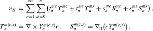
 are the radial MF and SV, respectively, and vH is the flow velocity, with subscript H denoting the horizontal components (θ, ϕ). Core surface flow modelling is an inverse problem to estimate a configuration of the flow vH that meets downward continued geomagnetic field models Br and
  on S(c).
It is well known that the flow computation using eq. (1) is, in principle, subject to a non-uniqueness problem (Backus 1968; Bloxham & Jackson 1991). There is generally a null-space in the forward problem described by the equation that predicts  from vH, with a given Br; different core surface flows can generate an identical SV, when they interact with a radial MF prescribed at the CMB. A simplified example of the null-space may be provided by zonal toroidal core flows generating no SV in the presence of an axially symmetric MF. In this case, the SV can not resolve the zonal toroidal flow component. In addition to this theoretical non-uniqueness, the practical flow inversion is subject to a further ambiguity originating from the variance of the SV model used as data. The true core flow may have components generating a SV signal not larger than the error level of the SV model. For such flow components, the SV model associated with finite variance has only marginal resolution, and the computation for these flows, though theoretically possible, tends to be flawed by prohibitively large variance accompanying the result. The flows with this additional ambiguity can therefore be regarded as forming a subset of the flow space, which we refer to as ‘effective null-space’.
To get around the ambiguity problem of the flow inversion, a priori information has been introduced. One of the most plausible assumptions is that the core flow vH is in geostrophic balance in horizontal directions (Le Mouël 1984). This assumption, referred to as tangential geostrophy (TG) assumption, has been frequently employed in core flow modelling (e.g. Le Mouël et al. 1985; Gire & Le Mouël 1990; Jackson 1997). The TG assumption has been shown to reduce the theoretical non-uniqueness to considerable extent, with respect to previous MF models (Backus & Le Mouël 1986). Yet, there still remains a finite null-space. A simplified example of the remaining null-space would be the case with the axial dipole MF alone, where the TG flow would not at all be resolved. Therefore, TG flow models have still been constructed by determining the flow elements within the effective null-space with a certain regularization in the inversion process. Many of the previous models were obtained with the regularization that minimizes the kinetic energy or spatial roughness of solution flow (e.g. Bloxham & Jackson 1991). The TG flow models thus estimated are composed of robust and less robust parts; the former is well constrained directly by SV, and the latter belongs to the effective null-space and possibly contains spurious features caused by the regularization that does not correctly reflect the true flow (assumed in this paper to be in a TG balance).
Our present study aims at seeking the part of TG flows belonging to the effective null-space. We extract it from typical TG core surface flow models, estimated from SV models associated with large variances, such as those estimated from the ground-based observations with a very limited spatial distribution and measurement quality. Of course, the MF models are also subject to variances, which alter the null-space itself. They are, however, far from being formally treated (Jackson 1995). We here restrict ourselves to investigating the effective null-space for a given MF model with no variances, that is, under an assumption of the perfectly known MF, usually used in the core flow modellings and frozen-flux tests (e.g. Bloxham & Jackson 1991; Holme & Olsen 2006). It should still be of interest to figure out how and where the effective null-space manifests in the maps of time-dependent flow models, because knowing the uncertainty of inferred flow is also important for discussing subsequent implications for a variety of the core dynamics, for example, the polar vortices (Olson & Aurnou 1999), torsional oscillations (Zatman & Bloxham 1997) and dynamic core-mantle coupling (Holme 1998). The goal of our study is not necessarily to constrain flows in the effective null-space or to find out a best flow model, but to present an implication as to which part of TG flows inferred from historical magnetic models tends to be robust or not.
2 Null-Space Flow
In this section, we introduce the null-space of the forward problem given by eq. (1), in which the radial SV,  , is generated from the core surface flow vH, in the presence of the radial MF, BH, on S(c) (assumed to be perfectly known). We start with the pure null-space, a flow subspace whose elements generate no SV at all whereas we note that our study seeks flows in the effective null-space, a more relaxed flow subset. The pure null-space is just a subset of the effective null-space, but it is helpful to know the configuration of the pure null-space on S(c), when discussing the method and results of the present analysis.
 . On the null-flux curves defined by Br = 0, vΨH (resp. vΦH) has only the components tangent (resp. normal) to the curves. Indeed, the normal component of vΨH (resp. the tangent component of vΦH) vanishes there, according to the identity ∇H · (BrvΨH) = 0[resp. (r × ∇) · (BrvΦH) = 0]. The flow vΦH has been referred to as ‘eligible flow’. Likewise, let us call the element vΨH of the pure null-space ‘ineligible flow’.
Let C denote a space of the horizontal vector field vH over S(c). For a given Br, we have the decomposition C = CΦ + CΨ, where the eligible subspace CΦ and the ineligible subspace CΨ are the linear subspaces for vΦH and vΨH, respectively. The sign + denotes the direct sum. In other words, a given flow vH can be uniquely decomposed into vΦH and vΨH). Now, we regard eq. (1) as representing a linear mapping of C to a space M of the scalar field  over S(c). Let T denote this linear mapping (T: C → M), which is dependent on Br over S(c) alone. Then CΨ is the kernel of T. The image of T, here denoted by the SV subspace MΦ(⊂M), necessarily has the SV elements satisfying the Backus' surface integral conditions defined for every patch closed by a null-flux curve. Conversely, the eligible flow vΦH is calculated uniquely, if and only if a given
  on S(c) satisfies the conditions. There is, otherwise, no unique determination of vΦH from SV, because of the arbitrariness in separating
  into the part for MΦ and the rest.

 , if and only if
  satisfies an infinite set of integral conditions along the contours of ζ (Chulliat & Hulot 2001; Chulliat 2004). The other part vΨ(i)H, constrained by neither SV nor the TG condition, is the flow tangent to the closed contours of ζ within the region called ‘ambiguous patch’ (Fig. 1) and having, simultaneously, a constant velocity along such contours. The first term of eq. (4.19) of Chulliat (2004) gives the general expression of vΨ(i)H, which has been shown to meet the TG condition (3). After all, a given TG flow can be decomposed into two TG flows, vPH = vP(e)H + vP(i)H, where vP(e)H ≡ vΦH + vΨ(e)H and vP(i)H ≡ vΨ(i)H. The TG flow part vP(e)H has been referred to as ‘eligible TG flow’. Likewise, let us call the pure null-space TG flow vP(i)H‘ineligible TG flow’.
The ambiguous patch (grey area) at the CMB and the contour of ζ (≡ Br/cos θ) within it at 1980.0 calculated from gufm1 (solid curve). The lines of ζ = 0 are depicted in thick curve. The contour interval is 2 × 10⁴ nT.
It may be possible to invoke the ‘ineligible TG subspace’CP(i) such that vP(i)H∈CP(i)(⊂CP and ⊂CΨ). Then CP(i) is the kernel of the mapping Ttg: CP → M, dependent only on a given Br on S(c). Also, we have the ‘eligible TG subspace’CP(e) for vP(e)H, or a complementary space of CP(i) over CP (i.e. CP = CP(e) + CP(i)). Given Br over S(c), the linear subspaces CP(i) and CP(e) are uniquely specified. The image of Ttg, denoted here by the SV subspace MPΦ(⊂MΦ), has elements necessarily satisfying the integral conditions given by Chulliat & Hulot (2001). From a general  which does not necessarily meet the conditions, the eligible TG flow cannot be uniquely determined because of the arbitrariness in separating
  into the part for MPΦ and the rest.
Let us now come back to the effective null-space flow, by relaxing the null-space, allowing for the variance of SV models. The effective null-space flow is defined here as the flow (or the TG flow) that leads to the SV forming only a subset of MΦ (or MPΦ), with its elements having magnitudes below the level of the estimated variance of an observation-based SV model. Such a flow (or TG flow) may well be considered as belonging to the null-space of T (or Ttg) in a practical sense. We refer to this type of flow (resp. TG flow) as ‘extended ineligible flow’ (resp. ‘extended ineligible TG flow’), collectively with the pure null-space flow, that is, the ineligible flow vΨH (resp. the ineligible TG flow vP(i)H), and denote it by  (resp.
  ). Accordingly, the set of
  (resp.
  ) is referred to as ‘extended ineligible subset’ (resp. ‘extended ineligible TG subset’) and denoted by
  (resp.
  ). Note that
  and
and  are not linear spaces like CΨ and CP(i). The residual flow (resp. TG flow) generates SV above the level of the variance, referred to here as ‘reduced eligible flow’ (resp. ‘reduced eligible TG flow’) and denoted by
  (resp.
  ). Accordingly, the set of
  (resp.
  ) is referred to as ‘reduced eligible subset’ (resp. ‘reduced eligible TG subset’), and denoted by
  (resp.
  ). The terminology and symbol for the flows and their sets are listed in Table 1.
Symbols and terminology for the flow subsets and their elements.
3 Method
We describe our method to extract the extended ineligible TG flow  from a given TG flow model vPH here. We rely on an algebraic approach that analyses the linear mapping Ttg: Ctg → M in the spherical harmonic domain.
3.1 Spherical harmonic representation
Inversion for the core surface flow is often performed with a ‘spectral method’ (e.g. Bloxham & Jackson 1991). The observation equation is derived from eq. (1), in which all the relevant quantities are represented in terms of coefficient vectors and a matrix of finite dimension. Its derivation can be found in previous papers (e.g. Whaler 1986). In this subsection, we briefly describe the observation equation, regarding it as a linear algebraic representation of the mapping T or Ttg.
 for r ≥ c are expressed as
 (in nT yr−1). The (non-dimensional) potential field basis function Rm(c,s)n(r, θ, ϕ) with reference to the mean Earth radius a is given by
 for β1 ≠ β2 and for an arbitrary r. β1 and β2 represent a certain set of the indices n, m and (c, s), and 〈 ·, · 〉r denotes the inner product for a vector field F(r, θ, ϕ) over a spherical surface S(r) defined by
 for any β1 and β2, and
  and
and  for β1 ≠ β2.
 is the column vector of the SV Gauss coefficients
  the vector of flow coefficients tm(c,s)n and sm(c,s)n and A the matrix containing the MF information and connecting the SV and flow coefficients. Dimensions of
  and
and  are given by NSV = LSV(LSV + 2) and NFL = 2LFL(LFL + 2), respectively.
We consider that  and
and  , where
  is the N-dimensional Euclidean space, with its elements
  giving the inner product defined by
  (the superscript T denotes the transpose). Thus,
  is an element of SV in the spectral domain, corresponding to an element
  of the SV space M in the spatial domain spanned by the basis functions Rm(c,s)n with n ≤ LSV (eq. 5). Also,
  corresponds to an element vH of the flow space C spanned by the basis functions Tm(c,s)n and Sm(c,s)n with n ≤ LFL (eq. 7). The matrix
  is the truncated representation of the linear mapping T: C → M.


 denote the column vector of the coefficients wm(c,s)n (i.e.
  ). Then w corresponds to an element vPH of the TG flow space CP spanned by the basis functions Wm(c,s)n with n ≤ LFL. Because of the relation v = Qw, eq. (8) can be reduced to
 being the matrix representing the linear mapping Ttg: Ctg → M. Flows in the ageostrophic space CQ are thus eliminated in the modified observation equation above.
 , where
  . By renormalizing the basis function
  , the inner product identity
  can be established, using the correspondingly modified SV Gauss coefficient vector
  . The flow inner product in the spatial domain at the CMB is expanded as
  , where
  . Further, the TG flow inner product gives
  , where
  . By renormalizing the TG basis function
  , the inner product identity
  can be established, using the modified TG coefficient vector
  (the real matrix
  is always obtainable, because
  is positive definite). In the end, with respect to the new basis functions, eq. (9) is given by
 and
and  .
.3.2 Specifying extended ineligible TG flow ![graphic]()
 of
of  [we order them as λ1 ≥ λ2 ≥ ⋯≥λN ≥ 0, with N = min (NSV, NPFL)].
  represents a change of the basis function
 , where the coefficients βj (in nT yr−1) are calculated as
  . In the same way, V represents a change of the basis function
 , where the coefficients αj (in km yr−1) are calculated as
  . We refer to βjΠj and αjVj as ‘scaled eigenfunction’ for certain SV
  and TG flow vPH, respectively. The observation eq. (10) is reduced to βj = λjαj for all j for λj > 0, indicating the one-to-one mapping between the eigenfunctions Vj and Πj.
The maximum degree of non-zero SV is given by LSV = LFL + LMF, according to the selection rule of integrals involved in the elements of  . With this LSV, it is always true for any positive integer LMF that NSV−NPFL = LSV(LSV + 2) −L2FL > 0. Therefore, the kernel of the finite-dimensional matrix
  , representing the ineligible TG subspace CP(i), does not always exist. This kernel can be expressed only when the matrix is rank-deficient, which is a specific case such as with the MF consisting of zonal components alone. It is rather likely, with actual MF models, that
  , considering that the ineligible TG flow vP(i)H in the pure null-space CP(i) resides only within the ambiguous patches with disjointed distribution on S(c) (Fig. 1). Such a flow configuration cannot be represented by a truncated series of the TG flow bases with spherical harmonics. This is in contrast to the ineligible flow vΨH. The kernel of A can always be represented by a truncated series of the flow bases, if vH given by eq. (7) is truncated at degrees LFL > LMF− 1 + (2L2MF + 1)1/2, a condition derived from NSV < NFL with LSV = LFL + LMF (e.g. LFL ≥ 33 for LMF = 14).
 by dividing a given TG flow vPH as
 is not significant with respect to the variance of a SV model. Let
  and
and  denote the SVs predicted by
  and
and  , respectively, and
  denote a SV model based on observations. They are expanded as
 . At least, the selection should be made so that the condition for
  to be included in the ineligible TG subset
  may hold. We here set the condition quantitatively as
 , and
, and  , with the average variance
  of a SV model over S(a). It is to be noted that
  (and also
  ), and hence that
  , whichever value is selected for p.
4 Starting Models
 and SV coefficient vectors
  at 2.5 yr intervals from 1842.5 to 1987.5. For the starting TG flow vPH, from which the extended ineligible TG flow
  is to be extracted, we use time-series models estimated from these matrices
  and vectors
  . The models, truncated at LFL = 14, are obtained epoch by epoch as regularized least square solutions
  to eq. (9):
 is supposed to be NSV = 840 and NPFL = 196, but only the submatrices
  ) and
) and  ), where
  , are used in the above equation. The regularization with
  minimizes the spatial roughness of the solution (Bloxham 1988), and has often been used in previous flow modellings (e.g. Jackson 1997; Pais & Hulot 2000). With reference to the modified bases Rm(c,s)n* and Wm(c,s)n*, a solution
  equivalent to
  of eq. (13) is derived by
  .
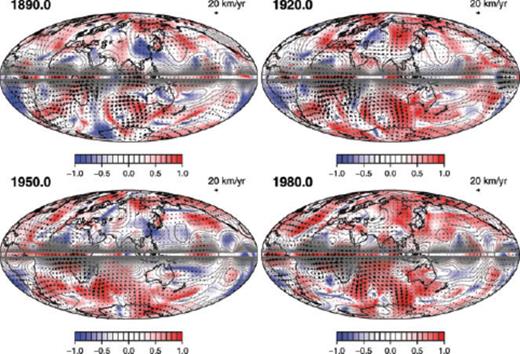
.Three TG flow models are obtained with different values for ξ: Optimal model; Smooth model and Rough model (see Table 2 for their statistics). For each model, we use a constant value of ξ to derive solutions at different epochs, based on the argument that the time variation of the SV variance has only a small effect on the solutions (Jackson 1997). The Optimal model, computed with ξ = 10−3, is considered more acceptable than the other two here, according to the trade-off curve between the misfit to the SV model and the spatial roughness of the solution. The maps of the Optimal model at several epochs are shown in Fig. 2. They are characteristic of strong westward flow below the southern Atlantic and retrograde vortex below the southern Indian Ocean, which are typical features of flow models inferred in previous studies (Bloxham & Jackson 1991).
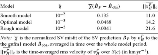
Statistics of the starting TG flow models vPH, estimated from the gufm1 model using eq. (13) with the various hyper parameters ξ (in nT2 km−2).
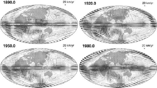
Maps of the Optimal model vPH at epochs 1890.0, 1920.0, 1950.0 and 1980.0.
An estimation of the SV variance  is needed to provide χC for the condition (12). A variance model coestimated in an individual field modelling could be somewhat optimistic, as it is just an estimate for a particular method and data set used in the modelling. A larger estimate of the variance might be made by investigating differences of independent models. We here simply assume a standard deviation of the SV Gauss coefficients given by
  at all epochs. This formula gives a linear dependence of
  on the spherical harmonic degrees l (≤14) in the logarithmic scale, and fits the standard deviation of the ufm1 SV coefficients at its earliest epoch 1840 (Jackson 1997). The ufm1 error diminishes by an order of magnitude for more recent epochs. However, the formula is also comparable to the difference between the ufm1 model and USGS model (Peddie & Fabiano 1982) at 1980.0 (see Fig. 1 of Pais & Hulot 2000). We consider that this formula gives pessimistic, but possible, SV errors for the later epochs, whereas still possibly optimistic for the earlier epochs. Assuming that there are no covariances among the SV coefficients, we obtain an estimate of the SV variance
  (n + 1) (2n + 1)10−0.2n + 1.0 = 5.5 × 10² nT2 yr−2, which corresponds to
  , the time average of χC over the relevant model period. Note here that the time-averaged SV square misfit of the Optimal model is about a half of this estimate of
  , whereas the misfit of the Smooth model is in excess of it (Table 2).
5 Analysis Results
5.1 Eigenfunctions
First, the singular value decomposition is applied to the matrices  . The singular values λj(j = 1, …, NPFL) are all non-zero at every relevant epoch (Fig. 3), as is expected from Section 3.2. All the basis functions Vj lead necessarily to non-zero SV, although a majority of them can be ineffective for SV production at the observationally detectable level because of the rapid decrease of λj with j. The singular value λj varies too smoothly with j to reasonably select a specific number for the effective rank p.
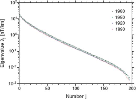
Eigenvalues λj(j = 1, …, 196) of the matrix Atg* at epochs 1890.0, 1920.0, 1950.0 and 1980.0.
The scaled TG flow eigenfunctions αjVj and SV eigenfunctions λjαjΠj are then calculated from the three starting TG flow models vPH. Fig. 4(a) shows ∥αjVj∥2c (= α2j) at 1980.0, that is, the energy distribution of the starting TG flows vPH over the eigenfunctions. αjVj associated with prominent energy are distributed randomly in j, and there seems to be no overall trend of ∥αjVj∥2c as a function of j. The three models tend to have similar energy for each eigenfunction with smallest numbers j, indicating the robustness of such flow part. On the other hand, the eigenfunctions with the larger j, having different energy for the different starting models, are affected seriously by the regularization. Fig. 4(b) shows  . The energy of the SV eigenfunctions clearly has a decreasing trend with increasing j, in accordance with the trend of λj. The most energy of the predicted SV is concentrated in the eigenfunctions with smaller j.
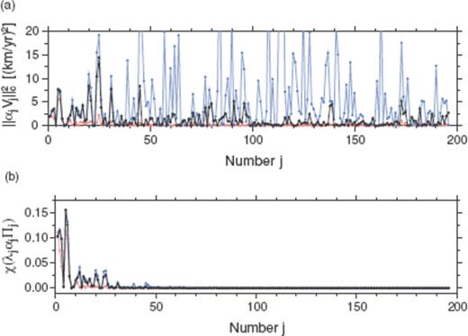
(a) Energy of the scaled TG flow eigenfunctions ∥αjVj∥2c at 1980.0. (b) Energy of the scaled SV eigenfunctions  at 1980.0 normalized by that of the gufm1 model
  . The coefficients αj are based on the Optimal model (black), Smooth model (red) and Rough model (blue).
Let us take a look at the maps of αjVj. Fig. 5 shows those with j = 5, 25, 91 and 173 from the Optimal model at 1980.0; these eigenfunctions have relatively large energy (Fig. 4a). The individual contributions of αjVj to the total flow vPH are very small, and each of their own configurations is not visually identifiable in the map of vPH (Fig. 2). αjVj with smaller j seem to have flows particularly dominant in the region where the magnitude of Br is larger, such as in the neighbourhood of the intensive flux spots around the equator below Africa. Furthermore, these flows tend to be normal to the contours of ζ. This kind of flow configuration is consistent with the analytical study of the eligible flow generating SV, as described in Section 2. On the contrary, αjVj with larger j have stronger flows in the region with smaller magnitude of Br, and they tend to be oriented along the contour of ζ. Unlike the ineligible TG flow vP(i)H, they do not necessarily have a constant magnitude along the closed contour of ζ, nor are they limited within the ambiguous patches. Nevertheless, each of them is very ineffective in generating SV, subject to the TG condition (3). These flow components can be admitted as the elements of extended ineligible TG subspace  , hardly constrained by SV in the practical TG flow inversion.
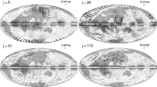
Maps of the scaled TG flow eigenfunctions αjVj(j = 5, 25, 91 and 173) for the Optimal model vPH at 1980.0, each satisfying the TG condition (3). Contours of ζ (= Br/cos θ) are also plotted.
We display in Fig. 6(a) the power spectra of αjVj from the Optimal model at 1980.0. They all show rather flat behaviours, with their powers at low degrees much smaller than those of the starting model vPH. Some of them even have powers greater than those of vPH at high degrees, implying the cancellation of small-scale flows when they are summed up to constitute vPH (eq. 11). This is attributed to the effect of the regularization imposed by the matrix  when computing vPH (eq. 13). Indeed, the TG flow eigenfunctions, both effective and ineffective to cause SV, should comprise a good amount of small-scale components. As seen in Fig. 5, they are conformed to the map of ζ having such a flat spectrum as Br has at r = c. In contrast to the power spectra of αjVj, those of their predictions λjαjΠj exhibit a systematic variation with j (Fig. 6b). Each spectrum peaks at a degree close to
  . The most robust flow components can therefore be identified simply with those that lead to the largest-scale SV. The scaled eigenfunctions at other epochs and from other starting models basically have the same characteristics in their maps and spectra.
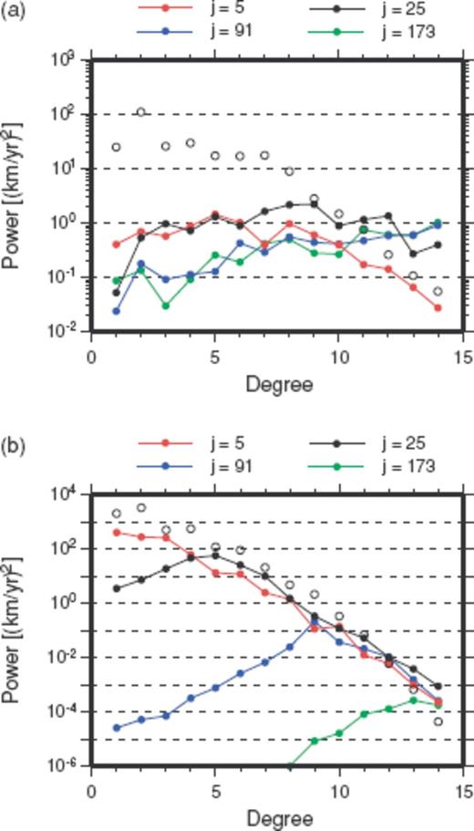
(a) Power spectra of the scaled TG flow eigenfunctions αjVj(j = 5, 25, 91 and 173) for the Optimal model vPH at 1980.0 (closed circle). Power spectrum of vPH itself is also plotted (open circle). (b) Power spectra of the scaled SV eigenfunctions λjαΠj(j = 5, 25, 91 and 173) at r = a at 1980.0 (closed circle). Power spectrum of the gufm1 SV model  at 1980.0 is also plotted (open circle).
5.2 Extended ineligible TG flow ![graphic]()
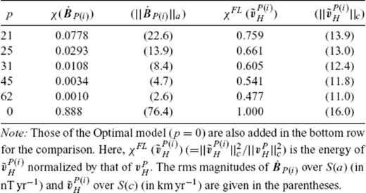
We start with extracting  from the Optimal model vPH at 1980.0. To see how it varies with the effective rank p selected for the decomposition (11), we here take various numbers, 21, 25, 31, 45 and 62, for p. The variation of
  with increasing p is associated with notable drops at these numbers, as the scaled SV eigenfunctions λjαjΠj have relatively large energy (Fig. 4b) at these numbers. The properties of
  for different p are listed in Table 3. The decrease of
  with p is remarkable compared with that of
  , although the condition (12) is satisfied for all the five cases (χC = 0.0893 at 1980.0). Their maps are shown in Fig. 7 (see Fig. 9 for p = 25). They have characteristic flows in common, such as the eastward flow along the equator below the western Pacific and westward flow below the southern Atlantic. This characteristic flow pattern emerges whichever number is used for p within its range in Table 3. We thus affirm that this typical flow configuration of
  is not primarily due to the robust eigenfunctions, that is, αjVj with smaller numbers j (say j≲ 62), but is basically due to those with larger j that are not robust. We note, nevertheless, that the flow features of the starting models vPH are not to be wholly attributed to either of
  or
or  . All that can be said is that vPH has some features that are relatively robust whereas others are not. Hereafter, we fix p to 25 for deriving representative estimates of
  and
and  from the Optimal model. This selection is based on a particularly significant drop or decrease around p = 25 in the variation of
  with p, which is observed continuously all through the model period.

Statistics of the extended ineligible TG flow  P(i)H extracted with various p from the Optimal model at 1980.0.
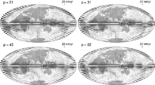
Maps of the extended ineligible TG flows  extracted from the Optimal model vPH at 1980.0, with respect to the reduced rank p = 21, 31, 45 and 62. Contours of ζ (= Br/cos θ) are also plotted.
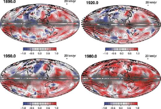
Maps of the extended ineligible TG flows  extracted with p = 25 at epochs 1890.0, 1920.0, 1950.0 and 1980.0. See Table 4 for their properties. Contours of ζ (= Br/cos θ) and the local vector coincidence index
  are also plotted.
Fig. 8(a) shows the spectra of  and
and  extracted with p = 25 from the Optimal model at 1980.0. The spectrum of
  indicates that it has much greater power at higher degrees than vPH. These small-scale flow components localize
  at particular regions or align it with the contour of ζ. Indeed, the powers of its prediction
  at lower degrees are very effectively reduced (Fig. 8b), whereas the powers of
  at lower degrees are not so significantly small as those of vPH. On the other hand, the spectrum of
  implies that largest-scale flows are not required to explain the SV model, although they can do the job, as indicated from the starting model. Note that, since the the small-scale flows can be replaced by the largest-scale flows, the spectrum of
  does not necessarily imply the necessity of small-scale flows for explaining the SV model.
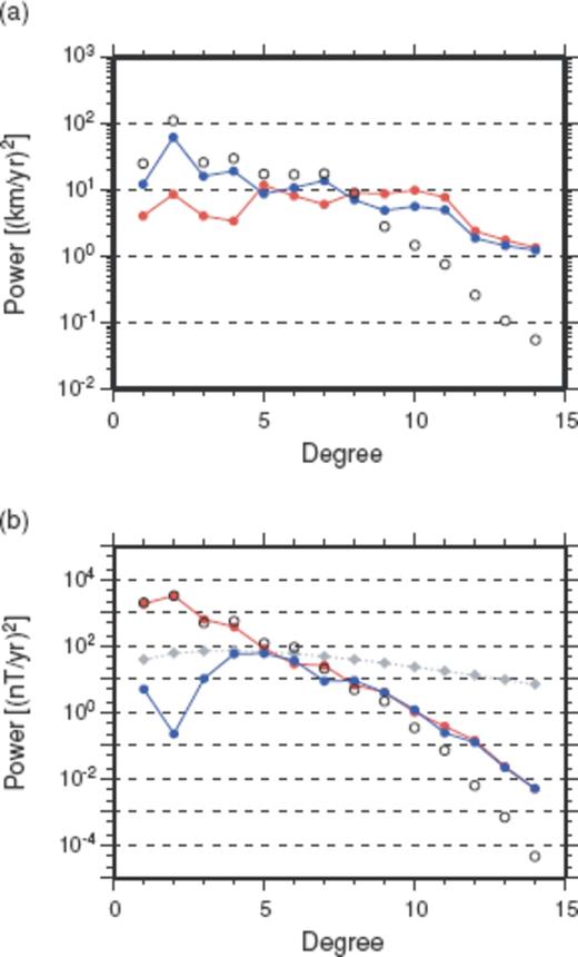
(a) Power spectra of the reduced eligible TG flow  (red closed circle) and effective ineligible TG flow
  (blue closed circle) extracted with p = 25 from the Optimal model vPH at 1980.0. Power spectrum of vPH is also plotted (black open circle). (b) Power spectrum of the SVs at r = a predicted by
  (red closed circle)
  (blue closed circle) at 1980.0. Power spectrum of the gufm1 SV model
  at 1980.0 is also plotted (black open circle). The SV powers predicted from
  are lower, or at least no higher, than those calculated from the SV error evaluated as
  nT2 yr−2 (grey diamond).
Fig. 9 shows the maps of  extracted from the Optimal model vPH with p = 25 at the epochs 1890.0, 1920.0, 1950.0 and 1980.0; the properties of these flows are given in Table 4. To better show the correlation of the two flow maps, we also plot in Fig. 9 the local vector coincidence index
  , which is defined for a certain point (θo, ϕo) on S(c)[see Appendix for the details of q, which varies from −1, when
  , to 1, when
  ]. These maps reveal that
  stands out primarily in the azimuthal direction, for any epoch, and consists of time-dependent and independent parts. The strong westward flow of
  below the southern Atlantic and South America agrees with that of vPH and appears to be a feature relatively persisting in time. On the other hand, there are some features appearing or disappearing: the retrograde vortex below North America at 1920.0 and 1980.0, the westward jet along the equator below Middle and South America at 1920.0 and the eastward jet below the western Pacific.
Statistics of the extended ineligible TG flow  P(i)H and reduced eligible TG flow
  P(e)H extracted with p = 25 from the Optimal model at various epochs.
Fig. 10 shows the maps of the reduced eligible TG flow  extracted from the Optimal model vPH at 1890.0, 1920.0, 1950.0 and 1980.0, together with
  ; their properties are given in Table 4. They are not as ‘optimal’ as vPH with reference to the SV misfit and flow smoothness in space but are still regarded as sufficiently compatible with the SV model. They have flow features consisting of vortices emerging mostly in the Southern Hemisphere, which are in contrast to the azimuthal jets typical of
  . They are also distinct from
  in that their configurations seem to be more or less steady in time. Table 4 indicates that the rms flow velocity of
  varies less significantly in time than that of
  . For example, the retrograde vortex below the southern Indian Ocean always exists in
  , which agrees largely with that of vPH. Most of the time-varying strong flows of vPH along the equator are not present in
  .
.
Maps of the reduced eligible TG flows  extracted with p = 25 at epochs 1890.0, 1920.0, 1950.0 and 1980.0. See Table 4 for their properties. Contours of ζ (= Br/cos θ) and the local vector coincidence index
  are also plotted.
We have made the same analysis with the other starting models vPH. The extracted flows,  and
and  , vary in accordance with the starting models and the effective rank p. Nevertheless, the basic configurations of
  , such as the prominent flow regions and orientations, are found similar to those in Fig. 10. Therefore, the representative maps of
  in Fig. 10 are regarded as depicting the general configuration of the robust part of vPH and those of
  in Fig. 9 depicting the residual part.
5.3 Zonal toroidal flow
Let us now focus on the zonal toroidal flow, given by the coefficients t0n(n = 1, …, LFL). We plot in Fig. 11 the three profiles of this flow component as a function of the latitude, each from the Optimal model vPH and its two parts  and
and  . The Optimal model has the notable westward circulations in the northern and southern polar regions at different epochs, which are referred to as polar vortices (Olson & Aurnou 1999). We find that these vortices are due largely to the robust flow
  , as clearly seen, for example, in the south (1950.0) or the north (1980.0). On the other hand, the contribution of
  seems dominating at the other latitudes, particularly around 30°S.
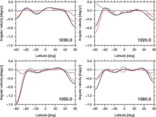
Axial angular velocities of the Optimal model vPH (black), the representative reduced eligible TG flow  (red) and the representative extended ineligible TG flow
  (blue) at 1890.0, 1920.0, 1950.0 and 1980.0.
 , as the above formula gives a linear function of the flow coefficients. We thus compare time evolutions of
  and
and  with the decadal variations of the observed excess LOD, here denoted by ΔLODobs.
Fig. 12 shows the time-series of ΔLODobs, together with those of ΔLOD(vPH) calculated from the Optimal model, Smooth model, and Rough model. As found out by Jackson (1997), ΔLOD(vPH) resulting from smoother flow model agrees the best with that of ΔLODobs, though we have not regarded this model as an optimal model. The Optimal model still makes a prediction moderately fitting the observation, but the Rough model does not, with its prediction having too large amplitudes. We also plot  and
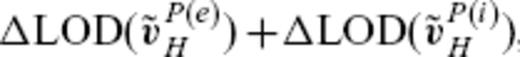
and  in Fig. 12. It is readily noted that
  is much better correlated to the observation than
  . The variations of the former are comparable in both amplitude and phase to that of ΔLODobs, regardless of the starting model. On the other hand, the variations of
  exhibit a poor correlation to those of ΔLODobs for any starting models. We can therefore conclude that the correlations between the variations of ΔLOD(vPH) and ΔLODobs, as seen in the cases with the Smooth and Optimal models [as well as many models in previous studies (e.g. Jackson et al. 1993)], are fortunately due to the robust part of the core flow. The extended ineligible TG flow
  does not seriously affect the computation of the CAM unless it is allowed to have a large energy like the Rough model.
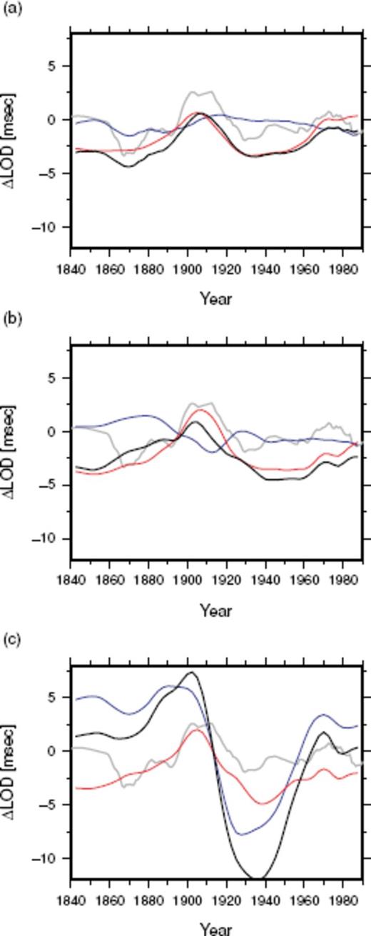
Decadal components of the excess LOD from the observation ΔLODobs (grey), and the LOD predictions from (a) the Smooth model, (b) the Optimal model and (c) the Rough model: ΔLOD(vPH) (black) from the starting model  (red) and
  (blue), from the representative reduced eligible TG flow
  and extended ineligible TG flow
  , respectively.
It is interesting to see how the coefficients t01 and t03 contribute to the variations of the LOD predictions. It has been shown that these coefficients vary in time in an anticorrelated manner, both presenting obvious extrema between 1910 and 1920 (Jackson 1997). This feature is also found in the Optimal model (Fig. 13). Our analysis reveals that these anticorrelated extrema are due not so much to the coefficients of  as to those of
  . There is even positive correlation between the variations of the two coefficients of
  . Their variations seem to be directly reflected to that of
  (Fig. 12b), showing peaks between 1900 and 1910. On the contrary, the variations of the two coefficients of
  are each similar to those of vPH regarding their amplitudes and anticorrelated behaviours. These coefficients of
  are allowed to be a major part of those of vPH, despite their rather minor contribution to the LOD predictions. This indicates that, even without any constraints on the CAM, the TG flow inversion, with a regularization as in eq. (13), tends to result in the anticorrelation of the two coefficients of
  , with their own angular momenta effectively cancelling each other.
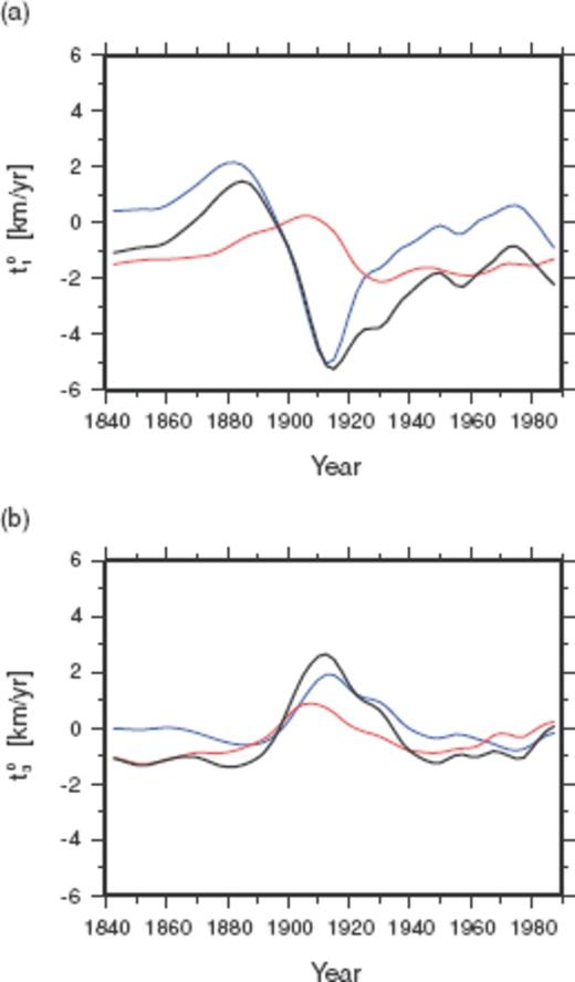
The flow coefficients (a) t01 and (b) t03 from the Optimal model vPH (black), and the representative reduced eligible TG flow  (red) and extended ineligible TG flow
  (blue).
6 Discussion
The presented examples of  exhibit the features shared by the starting TG flow model vPH. In what way are these large-scale configurations of
  selected in the process of the TG flow inversion? It is readily conceivable that
  is determined only passively, in such a way that the spatial roughness of total flow is diminished, that is,
  is configured to cancel out the roughness of the flow
  , soundly determined by SV. This passivity might answer why the representative maps of
  exhibits the remarkable time variations as seen in Fig. 9, whereas the local Br does not seem correspondingly variable. These flows are not directly resolved by local SV but are indirectly required in response to
  gradually evolving with Br in other regions.
It then follows that some conspicuous features of typical TG flow models may be recognized as possibly containing spurious flows resulting as a by-product of inappropriate regularizations. One notable example is the eastward jet along the equator, beneath the western Pacific, persistent in recent decades, which is obviously present in the both images of vPH and  around 1980.0. Minor relevance of SV to this jet may be suggested also by the flow models estimated without the TG assumption, which lack this eastward jet (e.g. Bloxham & Jackson 1991). Another example is the enhanced westward jet along the equator beneath South America, seen in the both maps of vPH and
  around 1920.0. It has been argued that the TG flow models tend to have larger energy around 1920.0, which may be responsible for the observation of correspondingly larger SV energy around the same epoch (Jackson 1997). Again, this strong jet itself is unlikely to be required directly by the local SV; it may be simply preferred by the given regularizations to be there with large magnitude, in accordance with the configuration of robust flows in other regions, which actually have a relatively large magnitude to account for the larger SV at these epochs.
Constraining the zonal toroidal flow and its time variations is one of the most important challenges in a long time-series core surface flow modelling. Estimated zonal toroidal flows can possibly reflect some important aspects of the core dynamics (e.g. Olson & Aurnou 1999; Hide et al. 2000; Pais & Hulot 2000). Our study has implied that the polar vortices of typical TG flow models are relatively well constrained by SV. This is probably due to the strong and relatively large-scale radial magnetic flux spots, such as below Siberia and North America. At mid- and low latitudes, zonal toroidal flow largely contains  , despite the presence of intensive flux spots around the equator. They are perhaps of too small-scale to lead efficiently to a large-scale SV above at the Earth's surface level, even if advected significantly by the local westward flow. Indeed, zonal toroidal flow alone plays only a minor role in generating SV (Gire & Le Mouël 1990). It is remarkable, nevertheless, that
  does not make a primary contribution to the prediction of the LOD variations, as shown for the Optimal model. It seems accidental that
  , which is azimuthally dominant and vigorously time-varying, leads to only minor CAM variations since no such constraint has been imposed in the inversion for the Optimal model. This finding is consistent with previous studies, demonstrating the stability of predicting the LOD variation from a wide range of flow models (Holme & Whaler 1998), or the resolution of the CAM being higher than those of the flow coefficients involved (Holme & Wardinski 2005).
Our results are also consistent with the demonstration of the TG flow inversion using synthetic field models resulting from numerical geodynamos (Rau et al. 2000). An example of spurious flow imaging is perhaps best seen in their inversion test with MF and SV, truncated at degrees similar to those in the practical inversions. The estimated TG flow has prominent azimuthal flows in the equatorial regions, which are not present in the dynamo flow (Fig. 11 of Rau et al. 2000). These flows seem to correspond to the representative maps of  in Fig. 9, despite the different MF arising from the dynamo. The false flow imaging occurs because of the a priori regularization in their inversion (with the matrix
  ) at odds with the dynamo flow, which has the power spectrum increasing with degree up to its peaks at degrees above 10. This observation can be interpreted as an aliasing due to the excessive damping of smaller scale flows, leading to spurious large scale flows that appear preferentially in the equatorial region, without generating SV signal practically detectable.
The false imaging of  could be avoided to a considerable extent, once the spectrum of the true core flow is known and one could specify an appropriate regularization in the inversion. Tests of TG flow inversion have been performed with a regularization in agreement with the spectrum of starting TG flows randomly synthesized (Eymin & Hulot 2005). They imply that a correct knowledge of the flow spectrum is actually useful for reducing the spurious part of
  in resulting model, especially those in the equatorial region (see their Fig. 14 for the distribution of flows free from serious contamination due to the false imaging). Though these flows are hardly determined alone by magnetic data plus the TG assumption, their resolution can be enhanced (or their variance can be lowered about the true flow) efficiently by reliable information about the spectrum. In other words, such flows are included in the effective null-space of Atg, but not in that of the resolution matrix R[≡ (AtgTC−1Atg + ξW−1)−1AtgTC−1Atg], defined by a proper regularization with W.
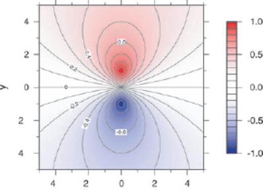
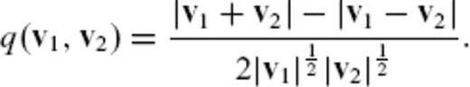
The local vector coincidence index q(v1, v2) as a function of v1 = (x, y) for v2 = (0, 1).
The tests of Eymin & Hulot (2005) point out, however, that a complete recovery of the true flow is still difficult, even if an appropriate damping is imposed. The true core flow can have elements belonging not only to the extended ineligible TG subset  but also to the null-space of
  , the latter of which is unavoidably caused by introducing the regularization itself. According to their analysis, small scale flows at high-latitudes might belong to this null-space (these flows should have already been absent in our starting TG flow models). In summary, the practical TG flow inversion can be understood as follows: (1) SV models resolve some of the TG core flow features belonging to the reduced eligible TG subset
  (such as a large part of the retrograde vortex below the southern Indian Ocean), but this robust flow is associated with high degree components that might not be present in the true flow; (2) a regularization appropriately imposed can be an effective aid for imaging a part of flows in
  , which are, if existent in the true core flow, prominent in the azimuthal component in the equatorial regions and (3) lack of resolution still remains for the true flows having small scale features at high-latitudes, which can be overdamped in TG flow inversions.
7 Conclusions
The radial frozen-flux induction equation at the CMB has been investigated in the spherical harmonic domain. The equation is considered as describing a linear mapping from the TG flow space to the SV space. Analysis of the representation matrix of the mapping allows a search for its effective null-space, a subset of the TG flow space, whose elements lead to a SV below its variance level. This approach does not generally resolve the pure null-space, which has already been fully discussed with the analytic studies in the spatial domain. Yet it is still useful for probing the effective null-space, for which one can simply rely on an algebraic analysis without any concern about the geometry of the field in the spatial domain. We have, thus, presented the flow part practically unconstrained by the SV model, which is accompanied by a certain amount of variance. This flow part is extracted from typical TG flow models by projecting them onto the effective null-space in such a way that it becomes orthogonal to the complementary part in terms of the kinetic flow energy integrated over the core surface.
The extracted flows at different epochs (1842.5-1987.5) suggest that a large fraction of flow emerging in a typical TG flow model may be manifestations of elements of the effective null-space. The kinetic energy of these flows occupies over a half of that of the given flow models, whereas the magnetic energy of SV predicted by them is no more than several per cent of that of the given SV models at the Earth's surface. These ambiguous flows extend outside the ambiguous patches and can be of large scale and large magnitude. In particular, strong azimuthal jets, which show up around the equator from time to time in typical time-series TG flow models, tend to fall in the effective null-space. They are in contrast to the vortices about the poles, which we find not largely involved in the effective null-space and hence being relatively well resolved by SV. Fortunately, the CAM computation and subsequent prediction of the LOD variation, which has been found correlated to the LOD observation, are attributed primarily to flows excluded from the effective null-space. The prediction is, nevertheless, not totally free from ambiguous flows in the effective null-space. Its uncertainty is apparently rather a critical issue in addressing a tighter fit to the LOD variations in the recent satellite flow modellings (Holme & Olsen 2006; Olsen & Mandea 2008).
In a long time-series TG flow inversion, it seems reasonable to impose some constraints on the solution with regard to its temporal variation, as the spurious flows can emerge especially in the part largely varying in time. Such constraints would effectively act on flows in the effective null-space, especially in a long time-series flow modelling, for which the SV variance is significant and an appropriate choice of regularization is not easily specified. This has been done by minimizing the temporal variation of the total flow energy (e.g. Holme 1998), but one may be able to minimize, as an alternative approach, the temporal variation of the flow spectrum, or consider appropriate degree of spatial smoothness independently for each epoch.
In this study, we have considered a large variance for the SV model in finding the robust and less robust TG flow parts. This model does not exceed its variance level at degrees higher than 6. The recent observations carried out by using satellites can considerably reduce the variance of magnetic models. Accordingly, TG flow models should become much better resolved, in which the extended ineligible TG flow is diminished. It would be interesting to see which flow features of the extended ineligible TG flow are the first to move to the reduced eligible TG flow, when it is attempted to fit a satellite SV model up to higher degrees.
Acknowledgments
SA thanks Richard Holme for useful discussions and suggestions. Two anonymous reviewers provided constructive and valuable comments, which greatly helped to improve the early version of the manuscript. Mioara Mandea is appreciated for carefully reading and correcting the manuscript during its revision.
References
Appendix
Appendix A: Local Vector Coincidence Index
