


Summary
We present new data that explores the link between pore pressure and seismic velocity to estimate the magnitude of the overpressure within the deep sediments of the Eastern Black Sea basin. New wide-angle seismic data, combined with coincident reflection data, have been modelled simultaneously using the seismic tomography code, Jive3D, to provide a well-constrained seismic velocity model of the sediments. Our models reveal a widespread low-velocity zone at the depth of 5.5–8.5 km, which is characterized by a velocity decrease from 3.5 to ∼2.5 km s−1. Using two separate methods that relate changes in seismic velocity to changes in effective stress, we estimate pore pressures of at least 160 MPa within the low-velocity zone. These pore pressures give λ★ values of 0.8–0.9 within the centre of the basin and above the Mid-Black Sea High. The low-velocity zone occurs within the Maikop formation, an organic-rich mud layer identified as the source of mud volcanism in the Black Sea and South Caspian Sea.
1 Introduction
An understanding of the pore-fluid pressure regime of a sedimentary basin can contribute to the determination of subsidence rates and depositional history, to the analysis of current tectonics and to estimates of hydrocarbon maturation and reservoir quality. Seismic velocity is intrinsically linked to the physical properties of the subsurface, and seismic data combined with borehole measurements can provide estimates of the magnitude and extent of pore-fluid pressures before drilling commences. This relationship between seismic velocity and pressure has been used to successfully estimate pore-fluid pressures in shallow (<4 km thick) sediments in locations such as the South Caspian Sea (Lee et al. 1999) and the Gulf of Mexico (Sayers et al. 2002). The Eastern Black Sea (EBS), is a deep rift basin with up to 9 km of sediments in the centre. Conventional multichannel seismic (MCS) reflection data cannot constrain accurate velocities within deep sediments (>4–6 km depth) due to limited source receiver offsets, and thus cannot be used to estimate pore pressures within this layer. Our data set combines wide-angle seismic data and coincident normal incidence data, to provide an accurate velocity structure for the entire sediment column. Combined with borehole constraints, we use velocity-stress relationships to estimate pore-pressures within the sedimentary infill of the EBS.
Pore pressures that are significantly higher than normal (overpressure), are caused by the inability of pore-fluids to escape as the surrounding mineral matrix compacts under the lithostatic pressure caused by overlying layers (Westbrook 1991; Wangen 1992; Mello et al. 1994; Swarbrick & Osborne 1998). There are a number of mechanisms that can cause overpressure to develop, and they can be grouped into three main types: changes in the stress regime, fluid volume changes and fluid movement. Stress related mechanisms can create considerable overpressures in rapidly subsiding basins through disequilibrium compaction, where the burial rates of the sediments are so great that the expulsion of pore-fluids is not sufficiently rapid to maintain hydrostatic pressure. This mechanism is thought to be the dominant cause of overpressures in the Gulf of Mexico (Berhmann et al. 2006) and South Caspian Sea (Lee et al. 1999). Lateral compression acts to reduce pore volume and thus increase pore-pressure. Rapid creation and release of pressure along faults is characteristic of this mechanism and is thought to be responsible for changing magnitudes of overpressure within accretionary wedges (Davis et al. 1983).
Volume increase of pore-fluids due to thermal expansion, dehydration of clays or hydrocarbon maturation, is another important mechanism. Expansion of pore-fluids as they are heated can produce small overpressures, but the volume increase is small (Luo & Vasseur 1992). Under certain conditions the dehydration of clays (smectite-to-illite), releasing water molecules into pore spaces, can also occur (Burst 1969), but both these mechanisms are unlikely to create significant overpressures as they require very low permeability in the overlying formation (Osborne & Swarbrick 1997). However, a consequence of clay dehydration is cementation, effectively increasing the sealing capacity of the layer (Hunt 1990). The tops of overpressured zones often coincide with zones of hydrocarbon generation, as the conversion from solid kerogen to liquid hydrocarbons, gas, residue and other by-products is accompanied by a volume increase (Mudford 1988; Hunt 1990; Hansom & Lee 2005). The generation of gas is thought to be accompanied by the largest volume expansion and is likely to create large overpressures. In nearly all abnormally pressured hydrocarbon accumulations, the fluid phase is gas (Law & Spencer 1998). Hydrocarbon generation can create large overpressures but occurs mainly as a secondary mechanism, helping to sustain large zones of overpressure generated by disequilibrium compaction in deep sedimentary basins (Swarbrick & Osborne 1998; Hansom & Lee 2005). Gas generation is thought to be a major secondary cause of overpressure in US Gulf Coast sediments (Hunt et al. 1994; Law & Spencer 1998), and many of the North Sea basins (Mudford 1988).
The most common cause of overpressure due to fluid motion is lateral variations is hydraulic head, where the elevation of the water table in highland regions exerts a pressure in the subsurface of shallow basins and can generate large overpressures if overlain by a seal. This mechanism is thought to generate significant pressures in the central United States Basin and Range province (Swarbrick & Osborne 1998). Pore-pressures can be transferred through the sediments in three dimensions, often redistributed directly beneath impermeable barriers. Motion along faults can release pore-fluids from an ovepressured zone creating overpressures at shallower depths. Ultimately, overpressure is a transient quality changing throughout time and space (Osborne & Swarbrick 1997; Law & Spencer 1998). Estimates of fluid pore-pressures are a snapshot of the current regime and overpressures would have been larger or smaller in the past.
Mud volcanism is a surface expression of overpressure, providing an important means of actively ventilating overpressured sediments, and is a clue to the magnitude and source of the overpressure (Dimitrov 2002; Yassir 2003). A sequence of low density, undercompacted overpressured sediments overlain by thick denser material, is mechanically unstable and is a characteristic feature of most mud volcano areas. There are three main triggers for mud volcanism: hydrofracturing caused by pore-pressures exceeding the overburden/lithostatic pressure, tectonic stress and extensional faulting that provide a pathway for overpressured fluids and seismic activity, which can weaken the overburden (Milkov 2000; Dimitrov 2002). Mud volcanoes are generally found along active plate boundaries and zones of compressional deformation, with more than 50 per cent of known mud volcanoes occurring along the Alpine-Himalayan active belt (Milkov 2000; Dimitrov 2002; Krastel et al. 2003; Yassir 2003). Some of the best studied mud volcanoes are located in the Mediterranean and Black Sea, and detailed analyses of their size, shape and fluid sources are given by Ivanov et al. (1996), Dimitrov (2002) and Kruglyakova et al. (2004).
2 Geological Setting
The Black Sea is a large, semi-isolated marine basin connected to the Mediterranean Sea by the Bosporus and the Sea of Marmara. The region has experienced several episodes of extensional and compressional tectonics since at least the Permian (Yilmaz et al. 1997; Robertson et al. 2004). Due to its location north of a group of orogenic belts linked to the closure of the Tethys, the Black Sea is generally considered to have formed by backarc extension (Zonenshain & le Pichon 1986; Okay et al. 1994; Spadini et al. 1997) but current deformation is compressional, due to the northward movement of the Arabian plate and westward escape of the Anatolian block (Barka & Reilinger 1997; McClusky et al. 2000; Reilinger et al. 2006).
The Black Sea has been a single deposition centre since the Pliocene (Robinson et al. 1996) but deep seismic reflection profiles reveal two separate basins that have distinct tectonic histories (Zonenshain & le Pichon 1986; Finetti et al. 1988; Okay et al. 1994). The major extensional phase, which caused the opening the of EBS basin has been widely discussed in the literature with different theories putting the basin opening during the Jurassic, Cretaceous (Zonenshain & le Pichon 1986; Okay et al. 1994; Nikishin et al. 2003), Palaeocene to early Eocene (Robinson et al. 1995b; Banks & Robinson 1997; Shillington et al. 2008) or Eocene (Kazmin et al. 2000). Post-rift, Cenozoic sediments make up the majority of the EBS infill (Finetti et al. 1988), with older pre-rift sediments identified on the shelf (Robinson et al. 1995a; Görür & Tüysüz 1997).
Upper Cretaceous, shallow-water carbonates appear to pre-date the main rifting event and are identified as the acoustic basement in the centre of the EBS basin (Zonenshain & le Pichon 1986; Finetti et al. 1988; Robinson et al. 1996; Görür & Tüysüz 1997). Upper Cretaceous to Early Palaeocene sediments comprise of clastic turbidites and chalks that are unconformably overlain by Late Eocene to Early Miocene mudstones. These muds are linked to the onset of anoxic conditions in the deep waters of the EBS and the sediments deposited were organic rich (Robinson et al. 1996). This mud-rich unit is known as the Maikop formation and the lowermost part of the sequence represents the most significant hydrocarbon source rock in the Black Sea region (Robinson et al. 1996). Very little sand is observed within this formation where it has been sampled offshore and seismic transparency within this layer suggests a homogeneous composition (Zonenshain & le Pichon 1986; Robinson et al. 1996). Early to Late Miocene sediments, sampled offshore Romania, comprise of mudstones (Robinson et al. 1995a; Spadini et al. 1996), with implied turbiditic layers observed in the seismic reflection profiles (Zonenshain & le Pichon 1986; Robinson et al. 1995a). Changes in water level and sediment drainage patterns, due to the uplift of the Carpathian Mountains during the Late Miocene, lead to the deposition of fluvial material and shallow-water limestones in this unit (Ross 1978; Robinson et al. 1996). The youngest sediments in the EBS, as recovered by gravity cores and drilling, comprise of clays with the occasional turbidite sequence (Ross 1978). The total thickness of top Cretaceous to recent sediment infill in the centre of the basin is 8–9 km (Shillington et al. 2008).
Mud volcanoes are a surface expression of overpressured sediments and Black Sea mud volcanoes have been extensively studied. The mud volcanoes can be found all along the continental shelf of the Black Sea (Kruglyakova et al. 2004) with a large concentration located in two specific areas: south of the Crimean Peninsula and within the Sorokin Trough (Ivanov et al. 1996; Dimitrov 2002; Krastel et al. 2003, Fig. 1). The volcanoes are distributed in water depths of 800–2200 m, are cone shaped and rise up to 120 m above the seafloor (Ivanov et al. 1996; Krastel et al. 2003). The source of mud volcanism is an overpressured layer (Dimitrov 2002; Yassir 2003), and the material brought to the surface by Black Sea mud volcanoes has very high gas saturation, with gas content of 80–99 per cent methane (Ivanov et al. 1996; Dimitrov 2002). Observations from seismic reflection profiles indicate that the roots of mud volcanoes in the Black Sea can be traced to ∼6 km depth and into the Maikop formation (Ivanov et al. 1996; Gaynanov et al. 1998). Clasts in the mud breccia brought up by these volcanoes also indicate the source is at least as deep as the Maikop formation (Ivanov et al. 1996; Gaynanov et al. 1998; Dimitrov 2002; Krastel et al. 2003). The Maikop formation extends throughout the Black Sea with a uniform thickness, but mud volcanism only occurs in a few locations. The Sorokin trough is considered the foredeep of the Crimean Alpine range (Krastel et al. 2003; Wallmann et al. 2006), while the sediments hosting mud volcanoes south of the Crimean Peninsula are raised by a crustal bulge (Finetti et al. 1988; Dimitrov 2002). Both locations are experiencing compression, which increases the overpressure and creates faults that provide an escape for the pressurized pore-fluids (Dimitrov 2002).
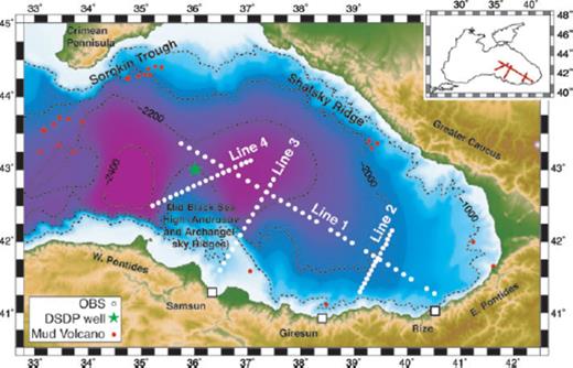
Map of the eastern Black Sea showing the location of the seismic experiment with elevation and bathymetry taken from GEBCO (IOC IHO BODC, 2003). The inset shows the location of the survey relative to the entire Black Sea. Positions of each OBS are shown as a white dot. Known locations of mud volcanoes are taken from Krastel et al. (2003), Ivanov et al. (1996) and Kruglyakova et al. (2004), and are shown as red dots. Other major features are also labelled and discussed further in the text.
3 Data Acquisition and Processing
3.1 Data collection
Wide-angle seismic data were collected onboard the RV Iskatel during 2005 February-March, using ocean bottom seismometers (OBS) provided by GeoPro GmbH. Each OBS holds a hydrophone and a three-component 4.5 Hz seismometer, operating at a 4 ms sample rate. The seismic source consisted of nine Bolt Long Life airguns towed at a depth of 9 m. The airguns were clustered so that their bubbles coalesced, and the total source volume was 51.5 L. Shots were triggered every 60 or 90 s from a stable clock (accurate to within under 1 ms) that was synchronized with onboard Global Positioning System (GPS). Data were acquired along four survey lines (Fig. 1, Table 1) positioned coincident or near-coincident with existing multichannel seismic (MCS) lines. Line 1 is ∼470 km long and extends from offshore Rize, across the centre of the basin, sampling some of the thickest sediments, and up onto the eastern flank of the Mid-Black Sea High (MBSH). Of the 34 OBS deployed, data were retrieved from 31 of these instruments. Lines 2 and 3 are oriented approximately parallel to the inferred direction of extension. Line 2 is ∼100 km long and extends from offshore Giresun to the centre of the basin. Line 3 is ∼160 km long and extends from offshore Samsun, across Sinop Trough, over the Archangelsky ridge, and into the centre of the eastern basin. Line 4 is ∼160 km long and crosses the MBSH where the Archangelsky and Andrusov ridges overlap. Data quality along Lines 1, 2 and 3 is very high, however, poor weather conditions experienced during the shooting for Lines 3 and 4 caused the vessel to slow down reducing the spatial shot interval from 180 to 110–150 m. Sea conditions were especially bad during the shooting for Line 4 and caused a decrease in the signal-to-noise ratio, which affected data quality. However, basement reflections can be identified on all OBS's along this line and data quality within the sedimentary arrivals remains high.
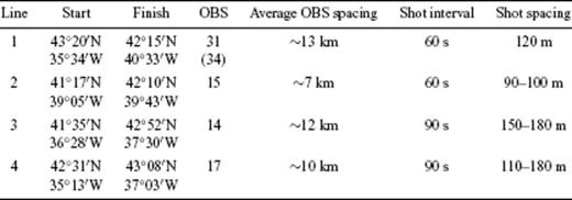
Details of wide-angle seismic data acquisition.
3.2 Data processing and phase picking
The location of each OBS was corrected for any drift from the deployment location during descent to the seabed. Traveltimes of the direct arrival travelling through the water from source to receiver were picked and assigned an error of 4–10 ms dependent on the signal-to-noise ratio. Correct locations for each OBS were found by minimizing the least-squares misfit between observed water-wave arrivals and those calculated using known bathymetry and a water velocity of 1.47 km s−1. This water velocity was found by forward-modelling the direct arrivals of three OBS whose positions were thought to be correct due to the symmetry of the direct arrivals about zero offset. The corrected locations of all OBS were within 500 m of the profile and were used to calculate new shot-receiver offsets for each OBS. Traveltimes were picked without applying a filter for offsets less than ∼30 km. For greater offsets a minimum-phase band-pass filter with corner frequencies of 3–5–15–20 Hz and an offset-dependent gain were applied in order to increase the signal-to-noise ratio. OBS data examples from all four survey lines, are shown in Fig. 2.
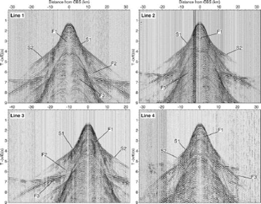
Examples of wide-angle seismic data recorded on an OBS taken from each survey line. The phases identified and picked to model the velocity structure are indicated. The x-axis represents offset from the location of each OBS. All plots have been filtered using a minimum-phase bandpass filter with corner frequencies of 3–5–17–21 Hz and traveltime has been reduced by 6.0 km s−1, such that arrivals with the apparent velocity of 6.0 km s−1 appear flat.
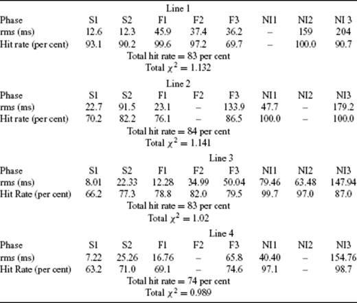
Along survey Lines 1 and 3, two main sediment refraction phases (S1 and S2) and three wide-angle reflections (F1, F2 and F3) were identified. Shallow sediment arrivals, S1, are usually observed at offsets of 4–8 km, and have a high apparent velocity gradient. F1 is a shallow reflection that corresponds to a change in the apparent velocity gradient between refracted phases S1 and S2. Mid-sediment arrivals, S2, are usually observed at offsets of 8–25 km and have a lower slope than S1. Beneath S2, an acoustic shadow zone and stepping back of later arrivals is observed on nearly all instruments along Lines 1 and 3. This feature is indicative of a low velocity zone (LVZ, velocity inversion) near the base of the sedimentary package. F2 is a weak reflection that marks the base of this LVZ, while F3 is a bright reflection identified as the top of the acoustic basement and the base of our sediment velocity models. Along survey Lines 2 and 4, the weak reflection F2 cannot be identified on most instruments and is not included in the models. An analysis of deeper, crustal phases is described by Shillington et al. (2009).
To constrain further the geometry of interfaces, normal incidence data from coincident or near-coincident reflection profiles were also picked. Survey Lines 2, 3 and 4 are coincident with existing industry reflection lines. Along Line 3, normal incidence horizons corresponding to F1, F2 and F3, denoted NI1, NI2 and NI3, respectively, have been picked (Fig. 3). Along Lines 2 and 4, normal incident horizons corresponding to F1 and F3 (NI1 and NI3) have been picked. Survey Line 1 does not directly coincide with existing industry MCS lines and normal incidence data has been picked along three different reflection lines, such that no pick lies more than 500 m from the wide-angle survey line. As Line 1 is not exactly coincident, the horizon corresponding to F1 has not been picked to avoid introducing any unnecessary traveltime errors from changes in horizon depth, but the horizons corresponding to F2 and F3 (NI2 and NI3) have been picked as any error in traveltime is well within the error assigned to the picks.
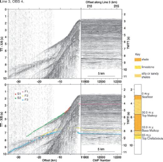
Wide-angle data, taken from OBS 4 on survey Line 3, plotted alongside its coincident reflection data. Traveltime picks of wide-angle phases and corresponding normal incident phases, are overlaid on the seismic data. A simplified stratigraphy, linked to key horizons in the seismic reflection data, is shown on the right-hand side.
In total, 13 681 wide-angle data picks and 747 normal incidence picks have been used to constrain Line 1, 8683 wide-angle data picks and 1120 normal incidence picks for Line 2, 18 427 wide-angle data picks and 1948 normal incidence picks for Line 3, and 18 100 wide-angle picks and 1118 normal incidence picks for Line 4. Each traveltime pick is assigned a picking error that generally increases with offset as signal-to-noise ratio decreases. The picking errors assigned to refracted phases were 20–24 and 25–44 ms for S1 and S2, respectively. The picking errors assigned to reflected phases were 48–60, 40–65 and 30–55 ms for F1, F2 and F3. Picking errors assigned to the normal incidence MCS picks were higher to account for differences in the location of the OBS and near-coincident MCS survey lines. Picking errors assigned to the normal incidence picks NI1, NI2 and NI3 were set to 80–90 ms.
4 Seismic Velocity Modelling
Seismic traveltime tomography is one of the most common methods for calculating seismic velocity structure. The simultaneous tomographic inversion of refracted rays, which tend to be best at constraining velocity variations, and reflected rays, which are better at constraining interface depth, results in a well constrained solution (Rawlinson & Sambridge 2003). Multiple refraction-reflection phase pairs can be identified in our data, so a seismic tomography model code that allowed simultaneous inversion of refraction and reflection traveltime data was sought. Two different codes, Tomo2D (Korenaga et al. 2000) and Jive3D (Hobro et al. 2003), were compared using a small section of Line 1. The comparison between these two codes is discussed in Appendix A. Based on this comparison, we decided to use Jive3D to model our data.
4.1 Model construction and parametrization
Using Jive3D, the seismic velocity structure of the sediments was modelled as a series of layers by inverting refraction, wide-angle reflection and normal incidence data simultaneously. The inversion process seeks a layer-interface minimum structure model that satisfactorily fits the data picks within their uncertainties. Model layers are mapped onto a fixed grid and interfaces, which are modelled as velocity discontinuities, are modelled as a function of lateral position. Layers are allowed to pinch out so that they only span part of the model. Ray-shooting is defined by a set of sources and receivers and ray shooting angles. This geometry links to traveltime data picks, which are divided into phases that describe the sequence of model layers through which each ray travels. To use a 3-D code to model our 2-D profiles, ray tracing parameters were set to trace only in the x-axis direction, and no variations are allowed in the y-axis direction.

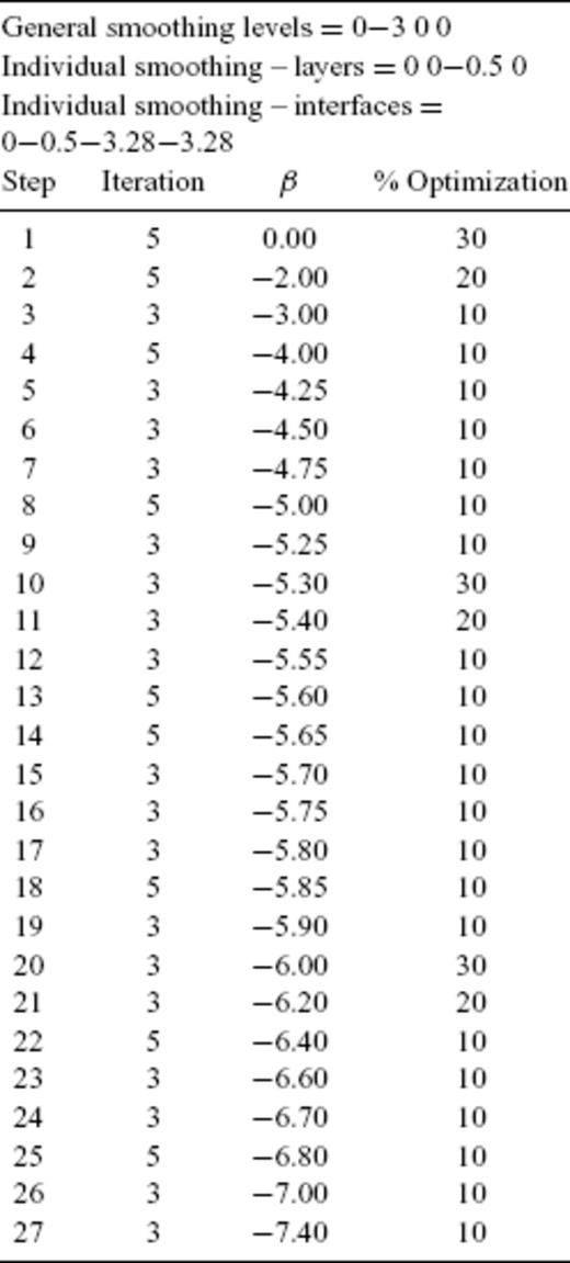
Sample Jive3D inversion pathway.
The final model produced by Jive3D does not depend on the starting model, and at the start of the modelling process, a range of starting velocity models were used to test this. Jive3D consistently produces a similar end model, and the starting velocity model used to produce the final results is shown in Fig. 4. Along survey Lines 1 and 3, four overlapping layers (to allow for interface movement) on a 1 × 1 km grid, defines the starting models. Model layer 1 spans 0–5 km and has a constant seismic velocity of 1.47 km s−1, representing the water column. Within this layer is interface 1, which is derived from the echo-sounder bathymetry collected during wide-angle seismic data acquisition. Neither layer velocity nor interface depth is changed during the modelling process. Model layer 2 spans 0–10 km with velocities increasing from 1.6 to 4.5 km s−1 and interface 2 defined as a horizontal boundary at 3.5 km depth. Data picks from phase S1 were inverted to find the velocity structure within this layer, while picks of reflected phase F1 were inverted to find the depth of the interface. Model layers 3 and 4 span 0–15 km with velocities increasing from 1.5 to 5.5 km s−1 and interface 3 defined as a flat boundary at 8 km depth and interface 4 defined as a flat boundary at 10 km depth. Data picks from phase S2 were inverted to find the velocity structure within the upper part of layer 3, while picks of reflected phase F2 were inverted to find the velocity in the lower part of this layer and the depth of interface 3. Data picks of reflected phase F3 were inverted to find depth of interface 4. Models for survey Lines 2 and 4 consist of three overlapping layers with similar structure: Layer 1 spanning 0–5 km, layer 2 spanning 0–10 km and layer three spanning 0–15 km. Data picks for refracted phase S1 were inverted to find the velocity structure of layer 2, while picks of reflected phase F1 were inverted to find the depth of interface 2. Phase S2 picks were inverted to find the velocity structure of the upper part of layer 3 and picks of phase F3 were used to find the velocity in the lower part of this layer and the depth of interface 3.
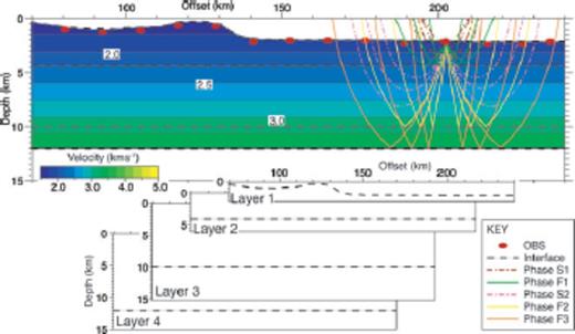
The starting velocity model used in the inversion of Line 3. The schematic aims to show how the starting model is comprised of four overlapping layers and interfaces. OBS locations along Line 3 are shown as red dots, with interfaces indicated by black dashed lines, and the velocity structure of the starting model is contoured every 0.25 km s−1. Overlaid on the starting model are example ray paths of the identified wide-angle phases, with reflections shown as solid lines and refractions shown as dotted lines.
4.2 Model results
The final sediment velocity models and traveltime residuals for survey lines 1, 2, 3 and 4 are shown in Fig. 5, while error statistics are given in Table 3 and resolution analysis is discussed in Appendix B. In the centre of the basin (130–420 km offset along Line 1 and 180–240 km offset along Line 3), the acoustic basement is relatively flat at ∼10 km depth and overlain by 8 km of sediments, modelled as three layers. Lines 1 and 3 both show similar velocity structure, and the comparison between the two survey lines where they intersect (368 km on Line 1 and 223 km on Line 3), is shown in Fig. 5. The shallowest layer (model layer 2) spans depths of 2–2.8 km and is characterized by a high velocity gradient. Velocities within this layer typically increase from 1.6 km s−1 at the seabed to 2 km s−1 at the base. The middle layer (model layer 3) spans depths of 2.8–8.5 km and is characterized by a lower velocity gradient and a widespread low velocity zone at its base. This widespread LVZ was consistently recovered at the base of model layer 3 during the modelling process. From 2.8 to 5 km depth the velocity increases from 2 to ∼3.5 km s−1 and the velocity then starts to decrease reaching a low of ∼2.5 km s−1 at 8.5 km depth. The lowest velocities are found at 230–320 km offset along Line 1, and 200–240 km offset along Line 3. The deepest modelled sedimentary layer (model layer 4) spans depths of 8.5–10 km and is characterized by low velocity gradient. Velocities in this layer increase from 3.4 to 3.8 km s−1.
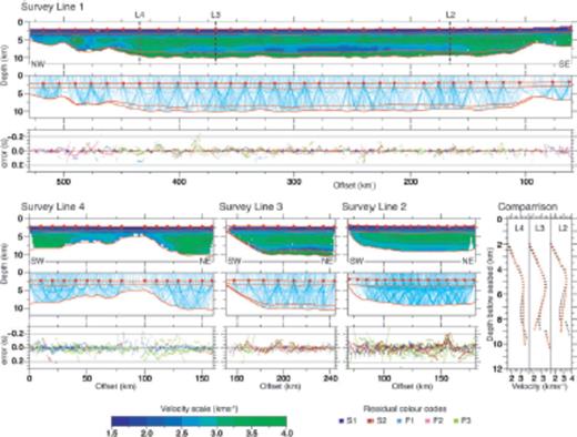
Final sedimentary velocity models for Lines 1, 2, 3 and 4, with 1-D comparisons at the overlap of Lines 2, 3 and 4 with Line 1. The location of the overlap between survey lines, are indicated by the vertical, black dashed lines in the Line 1 velocity structure plot. Each set of three plots show the velocity structure contoured every 0.25 km s−1 at the top, ray coverage decimated to every 13th ray in the centre plot, and traveltime residuals colour coded by phase at the bottom. The ray coverage and velocity structure plots are plotted with 3:1 vertical exaggeration. Red lines indicate modelled boundaries, red dots indicate the location of every OBS, blues lines are ray paths and black dashed lines represent zero and ±200 ms error in the residual plots. In the 1-D comparison plots, Line 1 is plotted as black crosses while Lines 2, 3 and 4 are plotted as red crosses.
Error statistics for velocity models of Lines 1, 2, 3 and 4.
Along Line 1, the deepest layer pinches out to the east at 100 km model distance, where the basement shallows towards the coast, and to the west at 460 km as the basement shallows at the edge of the MBSH. At the eastern end of Line 1 (60–100 km), the velocity within sedimentary layer 2, that spans depths of 2.4–6 km, increases from 2 km s−1 at the top, to 3.4 km s−1 at 4.8 km depth and then remains fairly constant to the base. At the western end of Line 1 (460–530 km offset), where the acoustic basement shallows towards the MBSH, the velocities within layer 2 are similar to those within the centre of the basin. Layer 2 spans depths of 2.9–8 km at 470 km and has a velocity that increases from 2 km s−1 at the top to 3.2 km s−1 at 5 km depth and then decreases to 2.6 km s−1 at the base of the layer. At 510 km offset the layer spans depths of 2.9–6 km with velocities increasing from 2 km s−1 at the top to 2.8 km s−1 at 4.5 km depth and then remains fairly constant to 6 km depth. At 150–170 km offset along Line 3, the basement shallows to ∼3.5 km at the edge of the MBSH, and the deepest layer pinches out. At 160 km offset, the velocity within layer 2, increases from 2 km s−1 at 2.8 km depth, to 3.1 km s−1 at ∼4.5 km depth.
The modelled sedimentary structure along Line 2 extends from 0–180 km model distance and crosses Line 1 at ∼117 km offset. The acoustic basement is relatively flat at ∼9.5 km depth in the centre of the basin and shallows to ∼7 km depth towards the coast. The sediments are ∼7.5 km thick and are modelled as two layers. The shallowest layer (model layer 2) corresponds to the top layer along Lines 1 and 3, with velocities typically increasing from 1.6 km s−1 at the seabed to 2 km s−1 at ∼2.8 km depth. The second layer (model layer 3) spans depths of 2.8–9.5 km and is characterized by a lower velocity gradient. Velocities within this layer typically increase from 2.0 km s−1 at the top of the layer to 3.4 km s−1 at ∼5 km depth. The velocity then decreases to ∼2.8 km s−1 at ∼8 km depth, before increasing to 3.2 km s−1 at the basement.
Line 4 is centred on the Mid Black Sea High, extending into the western and EBS basin, and the modelled acoustic basement topography is complex. At 0–28 km model distance, the basement is ∼8.5 km deep at the edge of the western Black Sea basin. At 30–70 km model distance the basement shallows above the MBSH to ∼6 km depth, and at 70–88 km the basement shallows abruptly to ∼4.5 km depth, before deepening again to ∼10 km depth at 100–132 km offset. At 132–160 km the basement in the eastern basin is relatively flat and the profile crosses Line 1 at ∼140 km offset. As with Line 2, the sedimentary structure is modelled as two layers. The first layer (model layer 2) corresponds to the top layer along survey Lines 1–3, with a velocity increasing from ∼1.6 to 2.0 km s−1 at ∼2.8 km depth. The velocity structure of the second layer (model layer 3) is more heterogeneous. In the western basin (0–30 km offset) there is a shallower velocity gradient, with velocities increasing from 2.0 to ∼3.2 km s−1 at 5.8 km depth. At ∼5.8–8.5 km depth the velocity is relatively constant at ∼3.2 km s−1. Above the MBSH (30–110 km offset) the velocity typically increases from 2.0 to ∼2.8 km s−1 at ∼5 km depth. The velocity then decreases to ∼2.5 km s−1 at the acoustic basement. In the eastern basin (110–160 km offset) the velocity structure is characterized by a shallower gradient, with velocities typically increasing from 2.0 to ∼3.5 km s−1 at ∼6 km depth. The velocity then decreases to ∼2.8 km s−1 at ∼9 km depth before increasing to ∼3.4 km s−1 at the acoustic basement.
4.3 Interpretation of sediment velocity structure
The top 2–3 km of sediments within the EBS basin have a relatively homogeneous seismic velocity structure. The velocity steadily increases with depth, with a vertical gradient of ∼0.7 s−1. For a shale lithology one would expect a velocity gradient in the upper sediments of ∼0.55 s−1, while for a sand lithology one would expect a velocity gradient of 1–1.15 s−1 (Japsen et al. 2007). A gradient of ∼0.7 s−1 suggests a shale-dominated lithology, which is supported by results from a DSDP borehole on the mid-Black Sea high (indicated on Fig. 1) that found the shallow sediments were mostly clays interrupted by occasional turbidites (Ross 1978). The seismic velocity structure of the deeper sediments is dominated by a widespread and fairly continuous low-velocity zone. The base of the LVZ is marked by model interface 3 and is constrained by seismic phases F2 and NI2 along survey Lines 1 and 3. The LVZ is ∼3 km thick, spanning the depths of ∼5.5–8.5 km and typically characterized by a velocity decrease from ∼3.5 to ∼2.5 km s−1 with lowest velocities of 2.3–2.4 km s−1 recovered around the centre of Line 1. This LVZ is sampled by a borehole located near the east coast of the EBS basin. The velocity structure sampled by this borehole indicates a similar decrease in seismic velocity, from 3.3 to 2.8 km s−1 (Fig. 9). Below the LVZ, the deepest sedimentary layer is ∼1 km thick with velocities returning to those modelled above the LVZ. This layer pinches out at the edges on the basin.
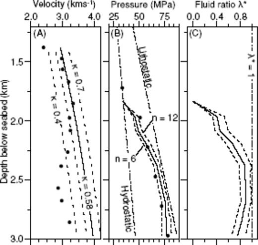
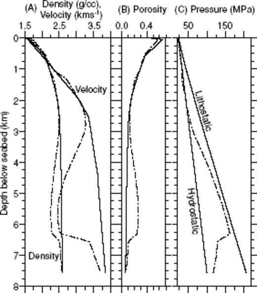
Seismic velocity and pore-pressure data measured at the borehole located near the east coast of the EBS. Plot (A) indicates observed velocity structure (dots) plotted with a series of compaction curves using α = 0.4, 0.5, 0.58, 0.7. Plot (B) shows lithostatic and hydrostatic pressure with measured pore-pressure values (dots) and estimates of pore-pressure using the Eaton method and values of n = 6, 8 and 12. Plot (C) shows the fluid ratio λ★ calculated using the pore-pressure estimates.
The top of the LVZ cannot be accurately constrained as we were unable to identify a corresponding reflection. However, along Line 1, a 90 per cent average hit rate is achieved for picks of seismic phase S2, which turns just above the LVZ. Our models predict the maximum offset refractions for the overlying sediments, and thus constrain the maximum thickness for the LVZ, which can be no thicker than the modelled thickness of ∼3 km. As the depth to the top of the LVZ cannot be constrained accurately, a trade-off exists between the thickness of this zone and its seismic velocity. A thicker zone with higher velocities will fit the model just as well as a thinner zone with lower velocities. Using the final model of Line 3, the effect of small perturbations to the thickness and seismic velocity of the LVZ on the error statistics of the model were tested. The LVZ thickness was perturbed by up to ±0.75 km, while the velocity was perturbed by up to ±0.2 km s−1. These models were run through the forward step of Jive3D, and the resulting χ2 and rms error values are shown in Fig. 6. This analysis shows that there is a single well-defined minimum and a perturbation of 0.1 km s−1, with a corresponding thickness perturbation, increases χ2 by ∼40 per cent.
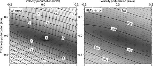
A contour plot showing how small perturbations in the modelled thickness and seismic velocity of the LVZ found on Line 3, effects the χ2 and rms error of the final Jive3D model. Thickness perturbations of ±.0, 0.1, 0.25, 0.5 and 0.75 km were tested in conjunction with velocity perturbations of ±0.05, 0.1, 0.15 and 0.2 km s−1, and each model run is represented by a circle. The contour plot on the left indicates the effect on χ2. while the contour plot on the right indicates the effect on rms error.
Due to the regularization and the lack of constraint on the top of the layer, the model indicates a smooth transition from velocities of 3.5 to 2.5 km s−1 over a depth of ∼2 km. This transition may in reality be sharper, but it is rare to achieve a perfect seal above a low-velocity, overpressured zone and a smooth transition from low to high seismic velocities is expected due to pressure leakage (Osborne & Swarbrick 1997). The regularization also affects horizontal variations in seismic velocity. The model parameters are set to force more horizontal to vertical velocity smoothing. In areas where the model is not well constrained, the regularization will produce a laterally smooth velocity structure, and this is true within the LVZ. To reduce this smoothing effect, the model was parametrized to allow greater roughness to emerge in the velocity structure of the layer that contains the LVZ.
The velocity contrast within the LVZ decreases to the SE along Line 1. At the intersection with Line 2 there is a velocity decrease from 3.4 to 2.8 km s−1 and further SE at 80 km model distance, velocities show a decrease from 3.4 to 2.9 km s−1. As shown along Line 4 and the NW end of Line 1, the magnitude of the LVZ above the Mid-Black Sea High is similar to that seen at the centre of the basin, typically showing a velocity decrease from 3.4 to 2.6–2.5 km s−1 at the acoustic basement. The contrast in lithology between the mud-rich Maikop formation and the overlying silty to sandy shales is unlikely to be sufficient to explain this magnitude of velocity decrease. A more likely explanation for a widespread LVZ within the EBS is an undercompacted sedimentary layer with elevated pore pressure.
5 Pore-Pressure Estimation from Seismic Velocities
5.1 Method
Seismic wave velocity in rocks increases during compaction due to the reduction in porosity and the increased grain contact. Fluid pore pressure is defined as the pressure within the fluids of the pore spaces within a rock. Under normal conditions, this fluid pore pressure should maintain communication with the surface during burial and thus should be at hydrostatic pressure (Bowers 2002). Any increase in pore-fluid pressure above the normal hydrostatic gradient reduces the amount of compaction that can occur and therefore decreases the seismic velocity. Most methods of pressure prediction assume that all measurable effects of a change in stress are a function only of the vertical effective stress (σeff). Effective stress is defined as the difference between overburden/lithostatic pressure (Lp, or pressure exerted by all overlying material, both solid and fluid) and hydrostatic pressure (Hp) for a given depth. Essentially effective stress is the amount of lithostatic pressure supported by the rock matrix (Bruce 2002; Sayers 2006). Seismic velocity increases with effective stress, thus any decrease in seismic velocity may be related to a decrease in effective stress and an increase in pore-pressure above hydrostatic. There are many different models that work on this principle. They commonly assume that porosity loss is primarily controlled by effective stress, that lithological and fluid variations have little effect on the velocity-stress relationship, and that local borehole data are available to calibrate coefficients (Gutierrez et al. 2006).


Pore pressures that are greater than total vertical stress, Lp(z), do exist temporarily in some basins but neither method can predict Pp greater than Lp. The Westbrook relationship predicts Pp = Lp when Vobs is equal to 1.50 km s−1. The Eaton relationship predicts Pp = Lp when Vobs is equal to zero.


A 1-D plot of the sedimentary structure at 250 km offset along Line 1. Plot (A) shows seismic velocity and density while plot (B) shows porosity calculated using eqs (4)–(6). The observed structure is shown as dashed lines, while Case 1 Vnorm, density and porosity, calculated using the same equations, are plotted as solid lines. Plot (C) shows Lp and Hp calculated using eqs (7) and (8) (solid lines) and Pp (dashed line) estimated using the Eaton method.
The implementation of the Eaton method of pore pressure prediction is straightforward, but Method 1 requires a normal velcoity at depth z′, to match every anomalous velocity at a depth z within the overpressured zone in order to estimate the pore pressure. The values are considered to match if the corresponding porosities differ by less than 0.01, which we consider an adequate match given the uncertainties in the velocities themselves.
5.2 Calculating Vnorm
Both methods require an assumption or prior knowledge of the velocity structure of sediments with a normal compaction history and hydrostatic pore pressures. In the EBS basin there are no borehole data for deep sediments that are not affected by overpressure, so assumptions are required. As so little is known directly about the lithology of the sediments in the EBS, two different simple assumptions have been made. The first assumption (Case 1) sets the observed velocity structure above the LVZ as normal. Within the LVZ, the normal velocity is interpolated between the observed velocity at the top of the LVZ, assumed for the purposes of this calculation to be at 4.5 km depth, and the observed velocity at the base of the sediments. Such an assumption will minimize the difference between the observed velocity profile and the ‘normal’ velocity profile, and thus will yield a minimum estimate of overpressure. Fig. 8(a) shows the normal velocity profile used for Case 1, plotted over 1-D plots of the observed sediment structure in the centre of the basin along all four survey lines.
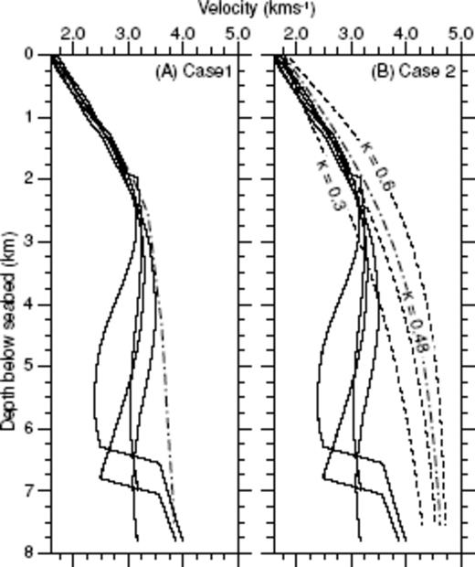
A plot showing the relationship between Vobs and Vnorm. Example 1-D profiles of the observed velocity structure, taken from all four survey lines are shown as solid lines. Case 1 Vnorm (dashed line) is shown in plot (A). Case 2 Vnorm is based on Athy compaction curves, and curves with compaction factors of κ = 0.3, 0.4 and 0.6 (dashed lines) are shown in plot (B). The Athy compaction curve with κ = 0.48 (thicker dashed line), represents Case 2 Vnorm.
5.3 Calibration
If borehole data are available, it is possible to find the optimal value for the exponent, n (in eq. 3),which relates Vobs to Vnorm, thus calibrating the Eaton method of pore-pressure estimation. Velocity and pore pressure measurements are taken from an industry borehole located near the east coast of the EBS basin, and are plotted in Figs 9(a) and (b). These measurements confirm a close association between reduced velocity and elevated pore pressures. In the LVZ, the measurements indicate a decrease in velocity from 3.3 to 2.8 km s−1 and an increase of pore pressure from 30 to 68 MPa. The easternmost part of the basin, where the borehole is located, is affected by compressional tectonics (Reilinger et al. 2006), bringing deep layers closer to the surface. To account for this compression, we have used a different compaction factor to calculate Vnorm. From Fig. 9(a), we can see that a curve calculated with a compaction factor α = 0.58, best fits the gradient of the shallower borehole velocity measurements, and this is set as Vnorm. The borehole pressures are estimated using the Eaton method and a range of predicted pore pressures, using different values of n, are shown in Fig. 9(b). To best match the pore pressure estimates to the observed borehole measurements, the exponent must be set to n = 8. This value was used to estimate pore pressures with the Eaton Method along all four survey lines.
5.4 Pore pressure results
Using the methods described above, the seismic velocity structure along all four survey lines has been used to estimate the pore pressure structure in the basin. Both methods yield similar results, differing by less than ±4–8 MPa. Because the Eaton method is more readily calibrated with borehole data, and our implementation of the method is more precise, only these results are discussed below. The estimated pore-pressure results and corresponding λ★ values are shown for all survey lines in Figs 10 and 11.
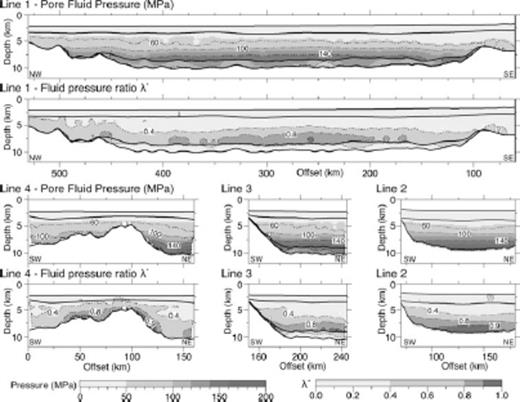
Using Case 1 to represent Vnorm, the final pore-pressure results, estimated using the Eaton method, and corresponding λ* values are shown. Each set of two plots show Pp in MPa on the top and λ* beneath. The Pp grids are contoured every 40 MPa (dashed lines), and the λ* grids are contoured at 0.4, 0.8 and 0.9 (dashed lines). Model interfaces are shown as solid black lines.
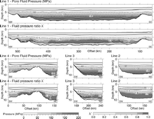
Using Case 2 to represent Vnorm, the final pore-pressure results, estimated using the Eaton method, and corresponding λ* values are shown. Each set of two plots show Pp in MPa on the top and λ* beneath. The Pp grids are contoured every 40 MPa (dashed lines), and the λ* grids are contoured at 0.4, 0.8 and 0.9 (dashed lines). Model interfaces are shown as solid black lines.
The overpressured zone, as implied by a large LVZ modelled in the seismic velocity profiles, is linked to a velocity decrease of 0.75–1.0 km s−1. Using eqs (4)–(6) this velocity decrease translates into a porosity increase from 10–13 per cent at 5.5 km depth to 24–30 per cent at 8.5 km depth in the centre of the basin. Using Case 1 to represent the Vnorm, the estimated pore-pressure structure is fairly continuous from the seabed to ∼6.2 km depth, with pore-pressure increasing from 22 to 100 MPa. The pressure gradient then increases significantly, reaching 160 MPa at ∼8.5 km depth, with highest pressures occurring in the centre of the basin between 220 and 410 km offsets (Fig. 10). At ∼8.5 km depth, lithostatic pressure is 170–172 MPa while hydrostatic pressure is 88 MPa, and the pressure ratio λ★ exceeds 0.8, reaching values of just over 0.9 above the MBSH. Using Case 2 to represent Vnorm, the estimated pore-pressure increases from 22 MPa at the surface to 100 MPa at ∼6.25 km depth. The gradient then increases and consistently reaches a maximum of 170–172 MPa at 8.5 km depth along the deepest parts of the basin. In this case, λ★ reaches values greater than 0.9 between 150 and 400 km offsets and above the MBSH (Fig. 11). Checkerboard tests of the velocity models (Appendix B) suggest that the vertical decrease in velocity associated with the LVZ is well resolved, with ±10 per cent perturbations, which correspond to pore pressure perturbations of ±2 MPa well recovered at a 2–3 km length scale. Horizontal variations in velocity of the same magnitude are only poorly resolved, even at a 30 km length scale.
6 Discussion
6.1 Sedimentary structure of the EBS basin
The final velocity models (Fig. 5) reveal a deep sedimentary basin, dominated by a thick LVZ at 6–8 km depth within the centre of the basin, and above the MBSH at 5–6 km depth. The LVZ indicates widespread overpressure linked to the Maikop formation, a result that is supported by the numerous mud volcanoes and gas/oil seeps located in the basin, which are shown to have origins in the Maikop (Ivanov et al. 1996; Gaynanov et al. 1998). Using wide-angle seismic data, in conjunction with normal incidence traveltime data, well-constrained seismic velocities for the entire thickness of the sedimentary column were determined. With accurate velocities and some borehole constraints, the link between changes in seismic velocity and a change in effective stress has been used to quantify the magnitude of pore pressures within the LVZ. This relationship is dependent on assumptions regarding the seismic profile of normally pressured sediments. As no constraints are available to make an accurate representation of the ‘normal’ seismic velocity structure of EBS basin sediments, we estimate pore pressures using two end-member models. Case 1 provided the smallest difference between the normal and observed velocities, such that the estimation of pore pressures will represent a minimum value, while Case 2 assumed a homogenous shale lithology (Fig. 9). Our results give a minimum estimate of pore pressure equal to 160 ± 2 MPa within the deepest sediments of the LVZ. The use of wide-angle data allowed us to constrain the deep velocity structure of the basin, which would not have been possible using standard multichannel seismic reflection data. Using this information, we were able to make pore-pressure estimates to quantify the spatial extent and magnitude of the overpressure within the EBS basin. This is an approach that could be easily applied to other regions, such as the complex overpressure regime in the South Caspian Sea and the US Gulf Coast sediments where overpressures reach 160 MPa at 8 km depth (Mello et al. 1994).
6.2 Origin and implications of the overpressure
The excess pore pressure may be expressed through the pressure ratio λ★ (eq. 9), and our results give λ★ values of at least 0.8 within the LVZ. When λ★ exceeds 1.0, the pore pressure can be great enough to fracture the overburden without requiring existing weaknesses, and allows the pore contents to escape to the surface. Although both methods of pore-pressure prediction cannot predict λ★ values of 1.0 or greater (for an observed velocity of >1.47 km s−1), there is no evidence for fracturing of the overburden within the centre of the basin. Therefore, if λ★ values exceed 1.0 anywhere, they do not exceed value sufficiently to overcome the cohesive strength of the sediment. Current pressure escape through mud volcanism and oil/gas seeps, can be found in certain locations around the edges of the EBS basin and onshore. Our models indicate that λ★ actually decreases towards the edges of the basin. This observation implies that the overburden is weakened by the current compressional tectonics, which facilitates fluid escape to the surface. This compressional deformation does not affect the centre of the basin, and the magnitude of overpressure alone within the LVZ is thus not great enough to fracture the overburden.
As shown in Fig. 12, the excess pore-pressures coincide with the Maikop formation as identified on MCS data, with the base of the overpressure lying at the base of the Maikop. The highest excess pore pressures exist within the Maikop. The top of the LVZ does not appear to parallel the stratigraphy, though limited resolution of the upper boundary means that we cannot rule out an association with a particular horizon, such as the top of the Maikop. Without a reflection to constrain directly the depth to the top of the LVZ, the velocity inversion is smoothed and the velocity within the LVZ is constrained only by the reflection F2 off its base or the reflection F3 beneath. Increased smoothing occurs in regions where the phase F2 has not been picked. Within the Maikop formation, the MCS data reveal numerous faults (Fig. 12, inset). These faults may have resulted from hydrofracture associated with past pressure release. These faults do not continue above the Maikop formation, indicating that any such hydrofracture did not propagate into the overlying sediments.
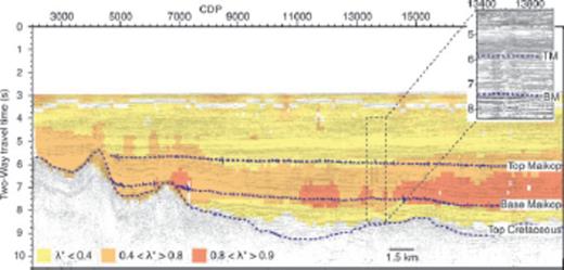
A plot showing the MCS reflection data, near-coincident with Line 1. The seismic data is overlaid by λ*, calculated from Pp values estimated using the Eaton method and Case 1 Vnorm. The inset shows an expanded section of the MCS data, illustrating the many small faults observed within the Maikop formation. On both plots, the blues lines represent Top Cretaceous, Base Maikop and Top Maikop, as identified on the MCS data.
The Maikop formation is a thick, homogenous layer of muds rich in organics deposited through Late Eocene to Early Miocene times. Rapid sedimentation, bypassing the margins and depositing straight into the centre of the basin, is thought to have occurred at this time (Robinson et al. 1995a). As the depositional rates are high, the major cause of excess pore pressure within this layer is likely disequilibrium compaction. Due to the high organic content, the formation is oil-prone (Robinson et al. 1995b), and analysis of mud volcanoes show deep thermogenic gas content (Kruglyakova et al. 2004). Hydrocarbon maturation within the Maikop could have provided a secondary boost to the magnitude of overpressure, possibly compensating for any pressure loss through the top of the overpressured zone. The size and magnitude of the LVZ, as imaged in the velocity profiles, indicates that the Maikop provides one of the most extensive overpressured zones in the world.
7 Conclusions
From our analysis of the seismic structure of the EBS basin and the link between changes in seismic velocity and changes in effective stress, we conclude that:
- (i)
Basin sediments have a maximum thickness of ∼8.5 km along our survey lines.
- (ii)
A widespread LVZ, spanning the depths of 5.5–8.5 km depth and indicated by a velocity decrease of 0.75–1.0 km s−1, has been identified as overpressure linked to the Maikop formation.
- (iii)
Depending on the choice of seismic velocity structure chosen to represent normal, the pore pressure reaches a maximum of 160–170 MPa in the centre of the basin. These pore pressures translate into values of λ★ greater than 0.8 within the centre of the basin and up over the MBSH.
- (iv)
A lack of mud volcanism and fluid/gas seeps in the centre of the basin suggests that λ★ does not exceed 1.0.
Acknowledgments
This work was supported by the Natural Environment Research Council (UK) (NER/T/S/2003/00114, NER/T/S/2003/00885, and a PhD studentship for CLS), BP and the Turkish Petroleum Company (TPAO). Ocean-bottom seismometers and airgun source were provided under contract by GeoPro GmbH. BP and TPAO generously provided access to the seismic reflection and well-log data that underpin this study. We would particularly like to thank G. Coskun (TPAO), A. Demirer (TPAO), R. O'Connor (BP), B. Peterson (BP), A. Price (BP), K. Raven (BP) and all those who sailed on the RV Iskatel for their help. We thank Graham Westbrook and an anonymous reviewer for constructive comments.
References
Appendices
Appendix A: Tomography Codes
We tested two model codes: Tomo2D (Korenaga et al. 2000) and Jive3D (Hobro et al. 2003). Tomo2D is a 2-D tomography code that completes regularized inversion of traveltime picks to solve for the velocity structure and the depth to one floating reflector (Korenaga et al. 2000). In this formulation, the starting model is a sheared mesh hung from the seafloor, and input picks are provided for first arrivals and one floating reflection (e.g. MOHO reflection (PmP) in many crustal applications for which this code was designed). Regularization is achieved through four parameters: (1) vertical and horizontal correlation lengths for velocity (i.e. smoothing parameters); (2) damping factors for velocity variation and reflection roughness. It is also possible to explore the trade-off between perturbations in velocity and depth by adjusting an additional relative weighting parameter of velocity and depth nodes. Successive iterations are performed to achieve a model with an acceptable fit. Because TOMO2D only inverts for one floating reflector, a layer-stripping approach must be used to model multiple pairs of reflections and refractions. Jive3D is a 3-D tomography code that is designed to simultaneously invert reflection and refraction traveltime data for multiple layers (Hobro et al. 2003). The code also uses a regularized inversion and flexible model parametrization to avoid dependence on a starting model. The inversion is regulated using smoothing parameters that determine the relative weighting of roughness applied individually to interfaces, layers and each spatial direction.
The test was done on a 250-km long section of Line 1 using data from a total of 12 instruments. A two-layer (water and sediments) example, test model A, and a three-layer (water, sediments and crust) example, test model B, were set up. Sediment refractions (phase S1 and S2) and the acoustic basement reflection (phase F3) were picked on all 12 OBS while crustal refractions and MOHO reflection were only picked on five central instruments so that crustal arrivals do not travel through unconstrained areas of the sediments. Both starting models were set up on a 1 × 1 km grid with smoothing parameters set so that the model will be four times smoother in the horizontal direction than in the vertical direction. The first layer, defining water velocity (1.47 km s−1) and the seabed, was held constant while we inverted for the second layer, which represents the sedimentary structure we inverted for. In test model B, a third layer, representing crustal structure was added. Jive3D was able to model layers 2 and 3 simultaneously, while Tomo2D used a layer stripping approach setting layer 2, as modelled in test A, constant whilst layer 3 was inverted for. The results for test models A and B are shown in Fig. A1 and show that both Jive3D and Tomo2D recover similar sedimentary structure with a maximum difference of less than 0.3 km s−1 between the well-constrained regions of the model. Because we are employing Tomo2D in a layer-stripping approach, the upper layers must be correct before modelling the deeper layers. If the structure is not correct, errors are propagated into the deeper section, and spurious velocities are introduced into the model. Anomalous high velocities are resolved by Tomo2D in the third layer of test model B (Fig. A1), and are caused by poorly constrained velocities at the edges of test model A, which introduce errors into the third layer. As we can identify several consistent sets of reflection/refraction pairs, we have chosen to use Jive3D for further modelling of this data set, as it will allow us to simultaneously model multiple layers. Simultaneously inverting for multiple layers allows information on shallow structure contained in deeper phases to be incorporated into the model and avoids the errors associated with a layer-stripping approach.
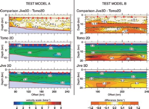
Test model results using Jive3D and Tomo2D tomography codes and the comparison (Jive3d minus Tomo2D) between them.
Appendix B: Resolution Analysis
A checkerboard method was used to show the resolution of the Jive3D traveltime inversion. A checkerboard of positive and negative velocity anomalies is superimposed onto the final sediment velocity model (Mfinal), and synthetic traveltimes are calculated. Using the same ray tracing and inversion parameters as those used in Mfinal, we inverted the synthetic traveltimes to find the synthetic model (Msynth), using Jive3D. The observed velocity model is then subtracted from the resolved synthetic model, (Mresolved), to show the checkerboard anomalies recovered by Jive3D. If checkerboard anomalies on a similar scale to features in Mfinal can be recovered, these features should be real (Rawlinson & Sambridge 2003).
Taking into account the modelled thickness of the LVZ and the scale of horizontal variations in velocity, five tests have been performed with checker sizes of 10 × 3 km, 20 × 3 km 30 × 3 km 10 × 2 km and 30 × 2 km. Each test has alternate velocity perturbations of ±10 per cent of Mfinal, which correspond to anomalies in the range of ±0.16 to ±0.36 km s−1. This checkerboard grid is added to Mfinal to create Msynth, which is then input into Jive3D as a starting model. Jive3D uses a B-splines method to sample the starting velocity model, which has a smoothing effect on the velocity structure. To account for this smoothing effect, the checkerboard we are trying to resolve is the one parametrized by Jive3D. The difference between the original input checkerboard and the sampled checkerboard is shown in Fig. B1. The sampling tends to smooth out every other checker in the row and highly distorts the checkers at the model interfaces, but for our purposes the sampled checkerboard is sufficient.
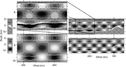
Checkerboard grids before and after B-spline sampling by Jive3D. The bottom plot shows the input checkerboard with dark colours indicating a negative anomaly, while lighter colours indicate a positive anomaly. The top plot shows the input checkerboard grid after Jive3D has sampled the input model. The colour scale is identical to the bottom plot, and the ±0.1 km s−1 contour of the original input checkerboard in overlaid on top of the sampled checkerboard. The inset shows a zoomed in section of the plot, to better show the effect of Jive3D sampling on the input checkerboard. On all plots, the white lines represent the modelled interfaces taken from the synthetic model.
Next we traced rays through Msynth with Jive3D to calculate synthetic traveltime picks. Random errors are generated within the assigned error bounds of the observed phase picks and added to the synthetic traveltime picks. Finally, Jive3D is run using the original starting model, inversion pathway and synthetic traveltime picks. As Line 1 has the coarsest source-receiver geometry and samples more of the sedimentary structure, the five tests are run on Line 1 and the results are shown in Fig. B2. It is assumed that the remaining survey lines will show similar or better resolution results than Line 1.
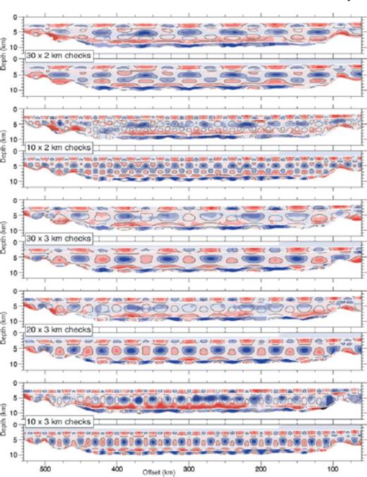
Checkerboard test results for Line 1. Each set of two plots showing the results of 10 × 3 km, 20 × 3 km, 30 × 3 km, 10 × 2 km, and 30 × 2 km checkerboard tests, with the resolved checks, (Mresolved−Msynth), on top and the input Msynth checks below. The ±0.1 km s−1 contour of the input checks are overlaid on both plots, to better illustrate how the checkers are resolved. On all plots, the white lines represent the modelled interfaces taken from the Mresolved.
The results show that within the top sedimentary layer (model layer 2) the 10 × 3 km and 10 × 2 km checkers are well resolved except at 90 km and 200 km model offsets that correspond to locations where there are large gaps between adjacent OBS. However, in these locations the 20 × 3 km checkers are well recovered. Above the LVZ within model layer 3, the 10-km and 20-km-wide checkers are poorly recovered in most areas whilst the 30-km-wide checkers are well recovered. Within the LVZ the 10 × 2 km, 10 × 3 km, 20 × 2 km and 30 × 2 km checks are not resolved, while the 20 × 3 km and 30 × 3 km checks are partly resolved. Below the LVZ, within model layer 4, the 10-km-wide checks are not resolved while the 20-km and 30-km-wide checks have been better resolved. The thickness of this layer does not exceed 2 km, so the vertical resolution is not assessed by our checkerboard tests. These results indicate that above the LVZ, vertical resolution is at least 2 km while horizontal resolution decreases from 10 km at the surface to 30 km at ∼7 km depth. Resolution within the LVZ is poor, which is expected as the velocity structure is only loosely constrained, and within the deepest sediments the horizontal resolution is at least 20 km.
Author notes
Now at: BG Group, Thames Valley Park, Reading RG6 1PT, UK
Now at: Lamont-Doherty Earth Observatory, Columbia University, Palisades, NY 10964, USA
