Constraints on shallow low-viscosity zones in Northern Europe from future GOCE gravity data

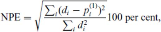
Summary

1 Introduction

During the last glacial maximum (LGM, ∼21 kyr BP) large parts of Northern Europe were glaciated. From field evidence and relative sea-level (RSL) curves, ice-load histories have been constructed (e.g. Lambeck et al. 1998; Peltier 2004) that cover the British Isles, Scandinavia and the Barents Sea and parts of continental Europe (e.g. Denmark, Poland) and the Kara Sea. This ice-load caused a sea level drop of about 15 m, out of a total of about 130 m, and a maximum depression of the Earth's surface of about 600 m in Northern Europe. Nowadays, almost the complete area is ice-free, but the land is still rebounding due to mantle flow toward the formerly glaciated areas. Using models of this process of glacial isostatic adjustment (GIA) and using RSL curves and geodetic data (especially GPS), inferences about the thickness of the lithosphere and the viscosity of the mantle have been derived for this area, either estimating the ice-load history in the same inversion (e.g. Lambeck et al. 1998) or using an existing ice-load history (e.g. Milne et al. 2004). For the latter, it should be kept in mind that the ice-load history is contaminated by information on the viscosity structure of the mantle, and that, in principle, the recovered viscosity structure is contaminated by the assumed ice-load history. Differences either reflect different a priori assumptions (e.g. thickness of the lithosphere, viscosity stratification of the mantle) or data that sample a different part in space or time. The difference in upper-mantle viscosity estimated by Lambeck et al. (1998) (3–4 × 10²⁰ Pa s) and Milne et al. (2004) (5 × 10²⁰–1 × 10²¹ Pa s), using the same RSES ice-load history of Lambeck et al. (1998), might, for example, be caused by non-linearity of the rheology, leading to a higher estimate of viscosity for inversions from ‘present-day’ GPS-data (Milne et al. 2004) than from ‘Holocene’ RSL-curves (Lambeck et al. 1998, Kurt Lambeck, private communication, 2006). Results from high-pressure and high-temperature laboratory experiments show that for high stress levels (>1−10 MPa) and/or large grain sizes (>100–1000 μm) most Earth materials show non-linear creep (e.g. Ranalli & Murphy 1987; Karato & Wu 1993), in which strain rate and stress are related by a power law, that is, the viscosity is stress-dependent. The reason most GIA studies still employ a linear rheology is that it greatly simplifies the mathematical formulation of the problem, and that it is successful in explaining different observations simultaneously (Wu 1992).

Another reason for the discrepancies between the result of Lambeck et al. (1998) and Milne et al. (2004) might be the different values they find for the lithospheric thickness (65–85 km, Lanbeck et al. 1998 versus larger than 90 km, Milne et al. 2004), because a combined thicker lithosphere and larger upper-mantle viscosity give a comparable quality of fit as a thinner lithosphere and smaller viscosity (Lambeck et al. 1998; Milne et al. 2004). This trade-off is partly due to the dampening effect of both a thicker lithosphere and a weaker shallow upper mantle and partly due to the relatively low spatial resolution of the RSL and GPS data, which, thus, only probe the medium- to long-wavelength signature of the induced field. This is confirmed by the low radial resolving power (∼200 km) in the shallow upper mantle (Milne et al. 2004) and by a reply of Lambeck & Johnston (2000) to a comment by Fjeldskaar (2000) on the lack of an asthenospheric low-viscosity zone (ALVZ) in the stratification of Lambeck et al. (1998). In this reply, Lambeck & Johnston (2000) state that such a low-viscosity region did not significantly improve the fit to the data in an earlier study for the British Isles, and that this, together with the relatively large uncertainties in the ice-load history, does not warrant a finer stratified earth model than the used three-layer model. The difficulty of constraining the viscosity of asthenosphere with RSL data in the presence of uncertainty in the thickness of the lithosphere is also found in laterally heterogeneous studies for Northern Europe (Kaufmann & Wu 2002; Martinec & Wolf 2005). The existence of an ALVZ is predicted from seismology, which show a ‘low-velocity zone’ (see e.g. Stein & Wysession 2003, p. 170) below the lithosphere. This zone is associated with ductile flow, because deformation laws, the convergence of the geotherm and the solidus and the strong vertical advection of deep heat from mantle convection predict low-viscosity material in this area (e.g. Stein & Wysession 2003, p. 204). From postseismic deformation studies in the western US, shallow upper mantle viscosities in the range of 10¹⁷–10¹⁹ Pa s are found (Pollitz 2003; Dixon et al. 2004). Steffen & Kaufmann (2005), using a comparable loading history as Lambeck et al. (1998), find some evidence for a low-viscosity region (10¹⁹–10²⁰ Pa s) in the Barents Sea area in a depth range of 160–200 km. However, no such region is found in Scandinavia, and no clear indication for such a region is found under the British Isles. Values for the lithospheric thickness range from 60 to 70 km beneath the Barents Sea and the British Isles to larger than 120 km beneath Scandinavia.

The thickness of the lithosphere and the viscosity of the asthenosphere are closely related to the thermal regime, which can for the lithospheric thickness be shown by comparing estimates of the ‘thermal thickness’ (Fig. 1a, Artemieva 2006) and ‘effective elastic thickness’ (EET, Fig. 1b, Pérez-Gussinyé. & Watts 2005). The former is determined from heatflow data and defined as the depth to 1300 °C, which is equal to the crossing of the conductive profile and the mantle adiabat (Artemieva & Mooney 2001, see also Section 2.1). The latter is determined from Bouguer gravity anomalies and flexure models of the lithosphere (Pérez-Gussinyé 2004). From Fig. 1, it is clear that both definitions show a large correlation, especially in Baltica, though in some areas, there are large discrepancies (e.g. Avalonia, see also Pérez-Gussinyé. & Watts 2005). In areas of relative high heatflow (or small thermal thicknesses) not only the asthenosphere but also the crust can show low-viscosity. Indications for such crustal low-viscosity zones (CLVZs) come from seismology, which shows lower crustal reflectivity in continental regions with relatively high (>70 mW m⁻²) heatflow (Meissner & Kusznir 1987), which indicates lamination supported by ductile flow. The viscosity depends on composition, fluid content and geotherm (Watts & Burov 2003; Ranalli & Murphy 1987) and can be as low as 10¹⁷ Pa s, as derived from postseismic (e.g. Hearn 2003) and mining-induced (e.g. Klein et al. 1997) deformation studies. Another indication of a weak lower crust is the rare seismicity within the lower crust. In terms of mechanical behaviour, seismicity is sampling an even shorter timescale of deformation than GIA studies sample. This rare seismicity means that intraplate earthquakes are mainly confined to the upper crust (0–20 km, Watts & Burov 2003; Ranalli & Murphy 1987) and the subcrustal mantle part of the lithosphere (Ranalli & Murphy 1987), which are thought to be brittle. Recently, this ‘jelly-sandwich’ model has been questioned in favour of a model in which all strength resides in the crust (see the discussion in De Meer et al. 2002; Jackson 2002), though this model seems to be possible only for a strong (dry mafic) lower crust and high surface heat flux (Afonso & Ranalli 2004). Some GIA studies, focusing on the vertical displacement (Klemann & Wolf 1999), present-day (Di Donato et al. 2000) and late-Holocene (Kendall et al. 2003) sea-level change and the global gravity field, as expected from GOCE (Vermeersen 2003; van der Wal et al. 2004), have included a CLVZ at a depth of 20–35 km, with a thickness of 10–15 km and a viscosity of 10¹⁷–10¹⁹ Pa s.

Figure 1.

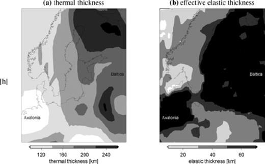
(a) Thermal thickness of the lithosphere (from Artemieva 2006) and (b) effective elastic thickness from Pérez-Gussinyé. & Watts (2005).

Open in new tabDownload slide

In recent GIA studies that include a laterally heterogeneous lithospheric thickness, the thickness variations are either deduced from seismic tomography models (e.g. Wu et al. 2005; Wang & Wu 2006) or derived from EET-estimates by multiplying with a constant (Zhong et al. 2003) or adding a constant (Pippa Whitehouse, private communication, 2007 Whitehouse et al. 2006). Lateral variations in mantle viscosity are usually derived from seismic tomography models and a certain scaling law (Latychev et al. 2005; Wu et al. 2005; Steffen et al. 2006; Wang & Wu 2006; Whitehouse et al. 2006). Here we derive the rheology of the crust and shallow upper mantle, to a depth of 220 km, from laboratory-derived creep laws for plagioclase feldspars (Rybacki & Dresen 2004) and olivine (Hirth & Kohlstedt 2003), with either a linear or non-linear rheology. Using creep laws the distinction between ‘lithospheric thickness’ and ‘asthenospheric viscosity’ is rather arbitrary, and we base the lithospheric thickness on a comparison of the timescale of the process and the Maxwell time of the Earth material, which is defined as the ratio of the viscosity to the rigidity (e.g. Ranalli 1995, p. 222). For timescales smaller than the Maxwell time, deformation is dominated by the elastic response, for timescales larger than the Maxwell time, by the viscous response. If we assume timescales for GIA of 10–100 kyr, we find that, using a rigidity of 68 GPa (Table 4), the shallow upper mantle (to a depth of ∼200 km) will be effectively elastic for a viscosity larger than about 10²³ Pa s. This viscosity-based lithospheric thickness estimate is closely related to thickness of the ‘rheological lithosphere’ (e.g. Kukkonen & Peltonen 1999; Pasquale et al. 2001; Ranalli 1995, p. 231), which is defined as the depth to a certain strength (e.g. 1 or 10 MPa) of the shallow upper mantle. Both definitions are not sensitive to the inclusion of shallow LVZs, in contrast to the EET, which is an integrated measure of the strength of the lithosphere. The EET can be estimated from GIA inversions (e.g. Lambeck et al. 1998; Milne et al. 2004), in which case, it defines the ‘short-term’ (10–100 kyr) elastic thickness (Martinec & Wolf 2005), or from inversions of gravity data (Bouguer coherence or free-air admittance studies, see Figs 1b and Pérez-Gussinyé 2004; Pérez-Gussinyé. & Watts 2005), in which case it defines the ‘long-term’ (>1 Myr) elastic thickness of the lithosphere. The short-term elastic thickness is larger than the long-term elastic thickness, because on the short timescales (10–100 kyr) involved in GIA, a high-viscosity (e.g. >10²³ Pa s) shallow mantle will not relax and is effectively elastic (Klemann & Wolf 1998). In the absence of shallow LVZs, the short-term elastic thickness should be comparable to the viscosity-based lithospheric thickness if the assumption of the threshold viscosity of 10²³ Pa s is correct. Note that the viscosity-based lithospheric thickness is smaller than the thermal thickness because a viscosity smaller than 10²³ Pa s can be reached in the conductive area.

Table 4.

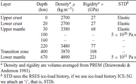
Earth stratification of the standard model.

Open in new tabDownload slide

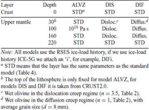
The upcoming Gravity field and steady-state Ocean Circulation Explorer (GOCE) satellite mission, planned for launch by ESA on 2009 March 16, is predicted to measure the static gravity field with centimetre accuracy at a resolution of 100 km or less (Visser et al. 2002). In previous work (Schotman et al. 2004; Schotman & Vermeersen 2005; Schotman et al. 2007), we have shown that geoid heights due to a CLVZ or ALVZ are above the performance of GOCE, and that GOCE is especially sensitive to the properties of a CLVZ, which shows maximum amplitudes from spherical harmonic degree 40–120 (∼500–150 km). The models we used were for ‘radially stratified’ (i.e. laterally homogeneous) earth models and linear rheology, which could be solved using a semi-analytical normal-mode technique (Vermeersen & Sabadini 1997; Schotman & Vermeersen 2005). Upon the introduction of lateral heterogeneities and non-linearity, the governing equations can no longer be solved using normal-mode techniques, and therefore we employ a FE model, based on the commercial package Abaqus (e.g. Wu 2004; Steffen et al. 2006; Schotman et al. 2008). As we are interested in high-resolution signals, the use of a global 3-D FE model (e.g. Wu et al. 2005; Wang & Wu 2006) is considered to be not feasible yet. In Schotman et al. (2008), we have shown that geoid height ‘perturbations’ computed from a flat 3-D FE model are very accurate. For CLVZs, these are generally smaller than 5 per cent and these differences are mainly short-wavelength ones. This is most likely related to our choice of elements (see table 2 in Schotman et al. 2008). For ALVZs, these are smaller than 10 percent and these differences are mainly long-wavelength ones. This is most likely due to the fact we take neither sphericity nor self-gravitation into account (again, see Table 2 in Schotman et al. 2008). Perturbations are differences between predictions from a ‘perturbed’ background model and predictions from the background model itself. The background model consists of a certain ‘Earth stratification’ and ‘loading history’. Here we assume that we know the laterally homogeneous background Earth stratification from 220 km downward from other GIA studies (e.g. Lambeck et al. 1998; Milne et al. 2004), and we test the sensitivity to the loading history by using two ice-load histories: RSES of Lambeck et al. (1998) and ICE-5G of Peltier (2004). We then consider perturbations due to creep laws for olivine in the shallow upper mantle and especially due to creep laws for plagioclase feldspars in the crust. For computation of the latter, we will use a suitable creep law for olivine in the shallow upper mantle of the background model. For this regional study, we do not consider gravity field signals due to chemically or thermally induced crustal mass inhomogeneities and, thus, use an isotropic crustal model.

Table 2.

Creep parameters for olivine (from Hirth & Kohlstedt 2003).

Open in new tabDownload slide

In Section 2, we start with describing the thermal and mechanical model. In Section 3, we discuss the laboratory-derived creep laws we use for the crust and mantle and estimate effective viscosities and lithospheric thicknesses. In Section 4, we apply the creep laws and predict geoid height perturbations for Northern Europe using the RSES ice-load history (Lambeck et al. 1998) and investigate the sensitivity to the ice-load history by using the ICE-5G load history of Peltier (2004). In Section 5, we then investigate to what extent GOCE is sensitive to composition and creep regime of the lower crust in Northern Europe, using estimated recovery errors for GOCE.

2 Thermomechanical Model

2.1 Thermal model

We estimate the temperature T in the lithosphere by solving the 1-D steady-state heat conduction equation (Meissener 1986, p. 126; Turcotte & Schubert 2002, p. 139), for which the solution for a multilayer model is (Liu & Zoback 1997):

1

with T_i, q_i, z_i the temperature in K, heatflow in W m⁻² and depth (i.e. positive in the downward direction) in m at the top of layer i+ 1 and k_i+1 and A_i+1 the thermal conductivity in W m⁻¹ K⁻¹ and heat production in W m⁻³ in layer i+ 1. The heatflow q_i can be computed from ‘Fourier's law’ (Turcotte & Schubert 2002, p. 132) and eq. (1) as

2

We compute the temperature downward from the surface heatflow q₀ and surface temperature T₀, using eqs (1) and (2). When the temperature in the mantle becomes close to the mantle solidus T_M heat transport is not controlled by conduction but by convection. In that case, the temperature follows an adiabatic temperature gradient equal to (Turcotte & Schubert 2002, p. 132)

3

where α_vc is the volumetric coefficient of thermal expansion (3 × 10⁻⁵ K⁻¹ for olivine, Inoue et al. 2004), ρ is the density and c_P is the specific heat at constant pressure (8 × 10² J kg⁻¹ K⁻¹ for olivine, Osako et al. 2004). If we solve this equation for T = T₁ at z = z₁, we get

4

We assume that heat transport is by conduction until the temperature is 0.85 T_M (Pollack & Chapman 1977) and that heat transport is by convection from T₁ = 1300 °C. In between, we assume that the temperature follows the 0.85 T_M contour, with the solidus T_M in °C given by (Hirschmann 2000, Table 2, Recommended Fit)

5

with P the lithostatic pressure in GPa.

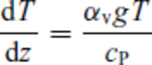
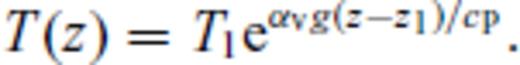
This might seem a rather crude assumption, but it compares well with a boundary layer between the purely conductive lithosphere and purely convecting asthenosphere, as proposed by Jaupart & Mareschal (1999). Following Jaupart & Mareschal (1999) and Artemieva & Mooney (2001), we can now define three lithospheric thicknesses (Fig. 2a): The boundary of the conductive layer (z₁, where the conductive geotherm crosses 0.85 times the solidus); the depth where the conductive profile crosses the adiabat at 1300 °C (z₂, ‘thermal thickness’, see Fig. 1(a) in Section 1), and the depth where the geotherm crosses the adiabat (z₃, ‘seismic thickness’), below which is a fully convective mantle.

Figure 2.

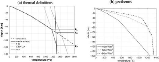
Thermal definitions of lithospheric thickness (a) and computed geotherms used in this study (b). In (a), ‘T_M’ is the solidus T_M as given by eq. (5).

Open in new tabDownload slide

Due to the depth dependence of heat generation and thermal conductivity, the results are sensitive to the assumed thickness of the crustal layers. By comparing heatflow measurements (Fig. 3a, based on the data set of Pollack et al. 1993 and for continental Europe on the extended set of Artemieva 2006) and estimates of crustal thickness (Fig. 3b, from CRUST2.0, http://mahi.ucsd.edu/Gabi/rem.dir/crust/crust2.html, accessed 2007 May 3), we estimate a representative crustal thickness of 40–50 km for ‘low’ heatflow (40 mW m⁻²), 30–40 km for ‘average’ heatflow (60 mW m⁻²) and 20–30 km for ‘high’ heatflow (80 mW m⁻²). In the computations of the geotherms, we take the upper values for each heatflow value, because the effect of the thickness within the limits is small. The values we use for heat production A and thermal conductivity k are given in Table 1. The values are based on a number of studies (Clauser & Huenges 1995; Jaupart & Mareschal 1999; Kaikkonen et al. 2000; Pasquale et al. 2001; Artemieva & Mooney 2001) and for heat production A on an exponential decay with depth in the crust (Turcotte & Schubert 2002, p. 141).

Figure 3.

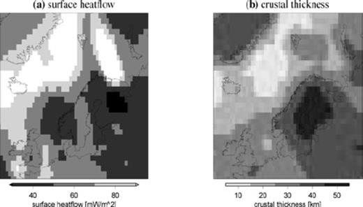
Surface heatflow (a) and crustal thickness (b) in Northern Europe. In (a), surface heatflow values are from Pollack et al. (1993), with an update for continental Europe by Artemieva & Mooney (2001). In (b), crustal thickness values are from CRUST2.0. The data sets are discretized to five levels and interpolated to a 1°× 1° grid.

Open in new tabDownload slide

Table 1.

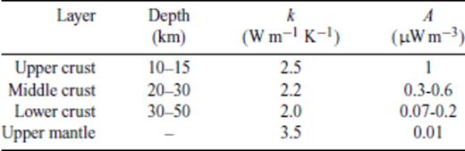
Parameters for thermal model.

Open in new tabDownload slide

The computed geotherms (Fig. 2b) for low, average and high heatflow compare well with Artemieva (2006). For example, our results show a thermal thickness (i.e. depth of the conductive profile to 1300 °C) for low heatflow of about 200–220 km, which also nicely fits the xenolith data of Kukkonen & Peltonen (1999). We expect the chosen heatflow values to be representative for our purposes, because values lower than 40 mW m⁻² are restricted to a small area in Finland (see Fig. 3a), and values larger than 80 mW m⁻² are restricted to oceanic areas, where the effect of changes in rheology are much smaller than in and just outside the ice-load areas. A notable exception is the Barents Sea, which is an area that has been glaciated in the past, though with large differences in the amplitude of the load between the RSES (Lambeck et al. 1998) and ICE-5G (Peltier 2004) ice-load histories (>1000 m, see Fig. 8b in Section 4), and where the value of 80 mW m⁻² is, on the basis of the available heatflow data, too low (Fig. 3b). In oceanic areas, which have a thin and mafic crust, we do not expect a ductile lower crust and as the effect of higher heatflows is small on mantle temperatures (see Fig. 2b), we can also use there a heatflow of 80 mW m⁻².

Figure 8.

RSES ice heights (a) and differences between ICE-5G and RSES ice heights (b) at LGM.

Open in new tabDownload slide

2.2 Mechanical model

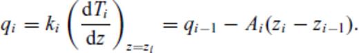
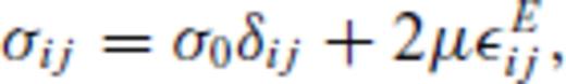
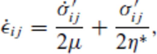
We will model the Earth as an incompressible, viscoelastic body, in which the total strain rate is the sum of the rate of change of the elastic strain ε^E_ij and creep strain ε^C_ij:

6

A linear relationship for ε^E_ij and the elements σ_ij of the Cauchy stress tensor is given by ‘Hooke's Law’, which is for an incompressible material equal to

7

with σ₀ the mean normal stress and μ the shear modulus or rigidity. For a linear viscous material, a similar relation holds:

8

with η the linear or Newtonian viscosity. Using the definition of the deviatoric stress (σ′_ij = σ_ij−σ⁰_ij, with σ⁰_ij = σ₀δ_ij) in eq. (6) gives

9

which is the constitutive equation for a Maxwell viscoelastic body.

Experimentally-derived creep laws for deformation in uniaxial stress have the form (Ranalli 1995, p. 77)

10

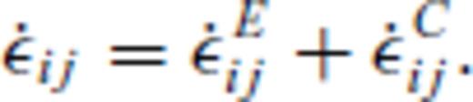
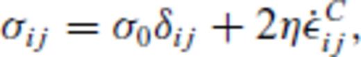
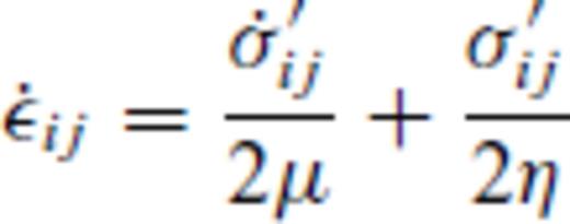
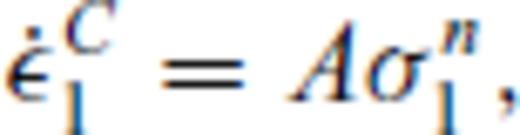
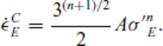
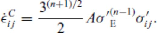
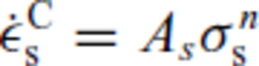
where σ₁ is the uniaxial stress and the corresponding creep strain rate. Note that A is, in general, a function of pressure, temperature and material properties, see Section 3. Using the definition of the effective deviatoric stress σ′_E and strain rate and their relation to the uniaxial stress σ₁ and strain rate (Ranalli 1995, p. 76)

11

we can write eq. (10) as (Ranalli 1995, p. 76)

12

If we now assume a linear dependence of the components of strain rate and stress deviator, then we can rewrite this equation to the following tensor form (Ranalli 1995, p. 77)

13

Using this relation in eq. (6), the constitutive equation for a material that is linear only in the elastic limit can now be written as

14

with η* the ‘effective’ viscosity defined as

15

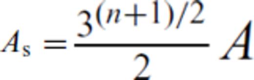
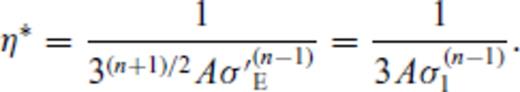
For a triaxial deformation experiment, we can use the same definition with the uniaxial stress σ₁ replaced by the stress difference σ₁−σ₃. For a deformation experiment in simple shear (, with σ_s the shear stress and the corresponding creep strain rate, compare with eq. 10), we get the following relation for the effective viscosity:

16

so that from comparing eq. (16) with eq. (15) it follows that .

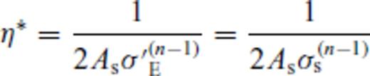
In this study, we use a flat, 3-D stratified deformation model based on the commercially available finite-element code Abaqus. For implementation of creep law parameters, Abaqus uses eq. (10) and the fact that the uniaxial stress is equal to the von Mises stress . With σ₁ replaced by , we can estimate effective viscosities from eq. (15) for applications that are not purely uniaxial as GIA. Note that Wu (1992) uses σ′_E instead of σ₁ (which differ by a factor , see eq. 11) in eq. (15), but this equation is not used in any computations with Abaqus.

The model has an 80 km horizontal resolution in the central area of 2920 × 2920 km², with a decreasing resolution outward to the edges at 10 000 km. In the vertical, the first 220 km is finely stratified (14 element layers), below which are five layers to model the deeper upper mantle and the lower mantle to a total depth of 10 000 km. The bottom of the model is fixed in all directions, and the sides of the model are fixed in the horizontal direction. The advection of pre-stress, which describes the restoring force of isostasy, is simulated using Winkler foundations, which act as springs to the bottom of a layer with spring constants proportional to the density contrast with the underlying layer (e.g. Wu 2004). We neglect the effect of self-gravitation, which is partly compensated by the lack of sphericity (Amelung & Wolf 1994) and which is shown to have a negligible effect on the accuracy of predictions for Northern Europe (Schotman et al. 2008). We compute geoid heights by solving Laplace's equation in the 2-D Fourier transformed domain, which gives accurate results compared with analytical, normal-mode methods (Schotman et al. 2008). We refer to Schotman (2008) and Schotman et al. (2008) for a validation and more extensive description of the model.

3 Composition and Creep Parameters

From high-pressure and high-temperature deformation experiments, rock materials show mainly two regimes of creep: grain size sensitive diffusion creep for low stress levels (<1–10 MPa) and/or small grain sizes (<100–1000 μm), and grains size insensitive dislocation creep for high stress levels and/or large grain size (Ranalli & Murphy 1987; Karato & Wu 1993). The stress levels induced by the Fennoscandian ice sheet (a few MPa, with a maximum larger than 10 MPa, see Wu 1992, 1995) are in the regime where the transition from diffusion to dislocation creep occurs.

In Sections 3.2 and 3.3, we show effective viscosities and yield strengths, where the latter is in the brittle regime equal to (Sibson 1974; Ranalli 1995, p. 248)

17

with P the lithostatic pressure at depth and λ the ratio of pore-fluid pressure to lithostatic pressure, taken to be 0.35 (Kaikkonen et al. 2000; Pasquale et al. 2001). This is based on the assumption that the pore-fluid pressure is equal to the hydrostatic pressure, which results in λ = ρ_W/ρ_E (Ranalli 1995, p. 248), with ρ_W the density of water and ρ_E the density of overlying material, assumed to be ρ_E = 2850 kg m⁻³. The factor α depends on the assumed kind of faulting, and following Pasquale et al. (2001), we assume that in the Baltic shield strike-slip faults are the most dominant, in which case α = 1.2 (Ranalli 1995, p. 248). This is intermediate between normal (minimum strength, α = 0.75) and thrust (maximum strength, α = 3) faulting (Ranalli 1995, p. 248). In the ductile regime, the yield strength σ^D₁ is related to the (effective) viscosity η* by

18

which follows from eqs (10) and (15). In intraplate regions, strain rates are typically larger than 10⁻¹⁸ s⁻¹ (∼10⁻¹⁰ yr⁻¹, Wu & Mazotti 2007; Pérez-Gussinyé 2004). Typical present-day rebound strain rates can be computed from measured horizontal and vertical velocities in Fennoscandia, which are in the order of 1 mm yr⁻¹ and 1 cm yr⁻¹, respectively (Milne et al. 2001). Using typical horizontal scales of 100 km and vertical scales of 1000 km, we arrive at maximum present-day strain rates of 1 mm yr⁻¹/100 km = 1 cm yr⁻¹/1000 km = 10⁻¹⁷ s⁻¹ (∼10⁻⁹ yr⁻¹), which is in agreement with findings of Wu & Mazotti (2007). As strain rates during glaciation and deglaciation might be higher, the value of 10⁻¹⁵ s⁻¹ estimated by Karato (1998) can be considered as an upper bound for GIA. We take therefore values of 3 × 10⁻¹⁵–3 × 10⁻²¹ s⁻¹, with 3 × 10⁻¹⁸ s⁻¹ as a typical value, where the factor 3 (actually 3.33) is included to simplify the translation from viscosity to strength with eq. (18) in the figures in Sections 3.2 and 3.3.

We first discuss in Section 3.1, the definition of the viscosity-based lithospheric thickness we use in this study. We then (Section 3.2) consider olivine creep laws for the shallow upper mantle and show effective viscosities and lithospheric thicknesses. In Section 3.3, we concentrate on plagioclase feldspars for the crust and show effective viscosities for different creep parameters and heatflow values.

3.1 Lithospheric thickness definitions

The viscoelastic strength of the lithosphere depends, among others, on the time-scale of the loading. The long-term strength is associated with the effective elastic thickness, as estimated from Bouguer coherence or free-air admittance studies (e.g. Pérez-Gussinyé 2004; Pérez-Gussinyé. & Watts 2005). It gives a thickness varying between a few km to thicknesses larger than 60 km, which is the upper bound with which the long-term elastic thickness can be derived with confidence (Pérez-Gussinyé. & Watts 2005). In Section 1, Fig. 1(b) we showed results obtained by Pérez-Gussinyé. & Watts (2005) for Northern Europe, using Bouguer gravity anomalies. As already mentioned in Section 1, the (short-term) elastic thickness in GIA is larger than the long-term elastic thickness, as we consider shorter timescales. For the timescales we are considering, we derived in Section 1, based on the Maxwell time, a viscosity at which the crust and mantle can be considered elastic of 10²³ Pa s. For geological timescales (>1 Myrs), this viscosity is larger than 10²⁵ Pa s. The viscosity-based lithospheric thickness thus defined is closely related to the ‘rheological’ thickness, which is defined based on certain yield stress (e.g. 1 or 10 MPa, Ranalli 1995, p. 231) and a certain strain rate. From eq. (18) we see that for a yield strength of 1 MPa the same viscosity (10²³ Pa s) is obtained using a strain rate of 3 × 10⁻¹⁸ s⁻¹, which nicely fits the assumption of this strain rate to be representative for GIA. Pasquale et al. (2001) estimate a rheological thickness of 110–140 km for the Baltic Shield based on a yield strength of 1 MPa and a strain rate of 10⁻¹⁵ s⁻¹, which corresponds, using eq. (18), to a viscosity of about 5 × 10²⁰ Pa s. This seems to be a very low viscosity for the lithosphere, except for processes with timescales smaller than a few hundred years as, for example, (post)seismic deformation. This is confirmed by the much smaller strain rates (<10⁻¹⁷ s⁻¹) assumed in shield areas by some other authors (e.g. Pérez-Gussinyé 2004; Wu & Mazotti 2007), which corresponds to viscosities larger than 5 × 10²² Pa s and a difference in rheological thickness of 20–40 km, as estimated from the variation of strength with depth as in Section 3.2. Kukkonen & Peltonen (1999) use the same strain rate as Pasquale et al. (2001) and a yield strength of 1–10 MPa to arrive at lithospheric thickness estimates of 130–185 km. They estimate a thickness variation of 15 km for one order of magnitude change in strain rate. The uncertainty in the rheological thickness of the lithosphere is, thus, dependent on the uncertainty in yield strength and strain rate, where for estimates based on viscosity, it is dependent on uncertainty in the timescale of the process. Note that the Maxwell time is a characteristic timescale of stress relaxation, which only provides a measure for which deformation mechanism (elastic, viscous) dominates for the assumption of a Maxwell viscoelastic earth. This means that there could be, for example, viscous deformation on timescales shorter than the Maxwell time also. Moreover, deviations from a Maxwell viscoelastic earth will lead to deviations in the characteristic timescale of stress relaxation.

3.2 Shallow upper mantle

For the upper mantle, the pre-exponential factor A in eq. (10) generally depends on temperature T, pressure P and grain size as well as water and melt content, as (Hirth & Kohlstedt 2003)

19

with E* and V* the activation energy in kJ mol⁻¹ and volume in 10⁻⁶ m³, respectively, A* a pre-exponential factor, d the grain size in μm, C_OH the water concentration as H/(10⁶Si), and m and r sensitivity parameters. The direct effect of melt is limited, provided melt contents remain small (less than a few percent); so, we have assumed negligible melt fraction. This assumption is probably reasonable even in the subridge mantle, where seismic and electrical conductivity results are consistent with relatively small melt fractions (Faul 2001; ten Grotenhuis et al. 2005). Melting can have a large indirect influence on rheology related to partitioning of water in the melt (Hirth & Kohlstedt 2003), resulting in an overall increase of viscosity associated with a change from wet to dry rheology in olivine.

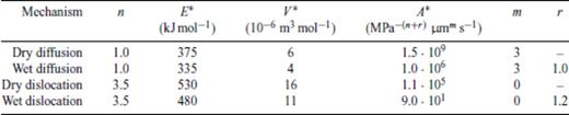
Material parameters can be found in literature (e.g. Karato & Wu 1993; Hirth & Kohlstedt 2003). We will use the recent compilation of Hirth & Kohlstedt (2003) for dry (C_OH omitted from eq. 19) and wet (C_OH = 1000) olivine in both the diffusion and dislocation creep regime (Table 2). The water content of C_OH = 1000 is taken from the estimate of Hirth & Kohlstedt (1996) for the sublithospheric mantle. For diffusion creep we take 8 mm as a typical grain size in the upper mantle and 1 mm as a lower and 15 mm as an upper boundary (Ave Lallemant et al. 1980; Dijkstra et al. 2002).

For low heatflow, in which the geotherm reaches the adiabat just below a depth of 200 km (compare with Fig. 2b), viscosities in the diffusion creep regime are given in Fig. 4(a). These curves can be computed using eq. (19) in eq. (10) and solving for the stress and computing the viscosity from eq. (18). If we compare the viscosity curves of Fig. 4(a) with results of GIA studies for Fennoscandia, we see that a grain size of 1 mm is not very likely in this area, as predicted viscosities are one to more than two orders of magnitudes smaller than the generally expected value of about 5 × 10²⁰ Pa s for the upper mantle (Lambeck et al. 1998; Milne et al. 2001) and a low-viscosity asthenosphere is not likely for cold areas as, for example, the Baltic Shield (Steffen & Kaufmann 2005). For larger grain size, a dry rheology seems to give too large viscosity values. However, if we define the lithospheric thickness as the depth where the viscosity is 10²³ Pa s (see previous section), we find a thickness for a dry rheology of 175–200 km, which is used for the Baltic Shield in some GIA studies (e.g. Wang & Wu 2006; Martinec & Wolf 2005) and which is close to the upper limit of 170 km found by Milne et al. (2001). For wet rheology and a grain size of 8 mm, we seem to get both a reasonable lithospheric thickness (140 km) and upper-mantle viscosity (3 × 10²⁰ Pa s).

Figure 4.

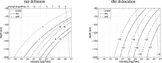
Viscosity estimates for ‘low’ heatflow (40 mW m⁻²) for olivine in the diffusion (a) and dislocation (b) creep regime. In (a), contour labels are grain size in mm, strength estimates are for . In (b), contour labels a are strain rates as 3 × 10^a s⁻¹. The brittle curves are computed from eq. (17) and the temperature profile used is from Fig. 2(b) (40 mW m⁻²).

Open in new tabDownload slide

For geological timescales (>1 Myr), the viscosity for which the mantle is effectively elastic was estimated in Section 3.1 to be larger than 10²⁵ Pa s, which gives Fig. 4(a) thicknesses smaller than 110 km. This is not in contradiction with the values found by Pérez-Gussinyé. & Watts (2005) for the long-term elastic thickness, because from EET studies, the largest thickness that can be found with confidence is about 70 km. Pérez-Gussinyé. & Watts (2005) find thicknesses for low heat flow (in general) that are larger than 70 km (see Fig. 1b). If we base the lithospheric thickness on the strength rather than the viscosity, the thickness of the lithosphere becomes strain-rate dependent. We then find from Fig. 4(a) that for a yield strength of 1 MPa (e.g. Pasquale et al. 2001) or 10 MPa (e.g. Kukkonen & Peltonen 1999), the rheological lithosphere has a thickness of 120–135 km. For a strain rate of 3 × 10⁻¹⁵ s⁻¹ (not shown), this increases to 185–210 km, and for a strain rate of 3 × 10⁻²¹ s⁻¹, this decreases to 80–90 km. We see from Fig. 4(a) that the rheological lithosphere compares well with the thickness associated with a viscosity of 10²³ Pa s for a strain rate of 3 × 10⁻¹⁸ s⁻¹ and with a viscosity larger than 10²⁵ Pa s for 3 × 10⁻²¹ s⁻¹.

For dislocation creep (Fig. 4b), it is difficult to combine a reasonable upper-mantle viscosity (10²⁰–10²¹ Pa s) with a reasonable lithospheric thickness (>90 km). Reasonable upper-mantle viscosities are only achieved for high strain rate (3 × 10⁻¹⁵ s⁻¹, ‘15’ in Fig. 4b), but then the viscosity-based lithospheric thickness (depth to 10²³ Pa s) is only realistic for a dry material (90 km, found as a lower boundary by Milne et al. 2001). However, for a strain rate of 3 × 10⁻¹⁸ s⁻¹, which is more common for present-day GIA, upper-mantle viscosities are very high (∼6 × 10²¹ Pa s for wet olivine), though then the viscosity-based lithospheric thickness of 125 km seems to be acceptable. The long-term thickness (depth to >10²⁵ Pa s) is smaller than 65 km, which is too small if we compare estimates of long-term elastic thickness (Fig. 1b) in areas of low heatflow (Fig. 3a).

For average heatflow (60 mW m⁻², Fig. 5), mantle viscosity shows a minimum where the temperature profile reaches the mantle adiabat at 120 km (compare with Fig. 2b). For diffusion creep (Fig. 5a) and small grain size (d = 1 mm), viscosities in the upper mantle seem again to be too low, especially for a wet rheology. Even if a viscosity of 5 × 10¹⁸ Pa s, as for dry composition, is reasonable, the very thin effective thickness (as determined by the depth to a viscosity of 10²³ Pa s) of 40 km seems unrealistic. For larger grain sizes (d = 8–15 mm), a dry rheology seems to predict too high values of viscosity. For a wet rheology and average to large grain size, the viscosity-based lithospheric thickness is about 60 km, which is not unrealistic for this heatflow, when compared with the results for the British Isles and the Barents Sea of Lambeck et al. (1998) and Steffen & Kaufmann (2005). The long-term thickness is then smaller than 50 km (end of the scale) and probably resides in the crust only. This would give, depending on the composition of the lower crust, lithospheric thickness estimates of 30–40 km, which seems quite realistic (compare Figs 1b and 3b). Note that in this case, we do not have a ‘jelly-sandwich’ because all long-term strength would reside in the crust, which is in line with predictions from Afonso & Ranalli (2004) for high heatflow. In Fig. 5(b), we show the viscosity for dislocation creep. The shallow mantle has viscosities as low as 10¹⁹ Pa s, but only for high strain rate (3 × 10⁻¹⁵ s⁻¹), whereas for lower strain rates, the viscosities seem to become too high. For high heatflow (80 mW m⁻²) the profiles are comparable to those for average heatflow, though with a somewhat lower viscosity to 75 km depth.

Figure 5.

Viscosity estimates for olivine and ‘average’ heatflow (60 mW m⁻²) for diffusion (a) and dislocation (b) creep. In (a), contour labels are grain size in mm, strength estimates are for . In (b), contour labels a are strain rates as 3 × 10^a s⁻¹. The brittle curves are computed from eq. (17) and the temperature profile used is from Fig. 2b (60 mW m⁻²).

Open in new tabDownload slide

We conclude that the creep law for a wet rheology in the diffusion creep regime with an average grain size is the most representative for Northern Europe, based on comparisons of predicted lithospheric thicknesses and upper-mantle viscosities with other studies for Northern Europe. We will therefore use this creep law (model DIF, see Table 4) as a reference for realistic predictions (Section 4) and use a wet rheology in the dislocation creep regime (model DIS, Table 4) to test the sensitivity to the background model of perturbations due to a ductile crustal layer.

3.3 Crust

For the crust, the pre-exponential factor A, as defined in Section 2.2eq. (10), generally depends on temperature T and grain size d (in μm), as

20

with Q* the activation energy, A* a pre-exponential factor and m a sensitivity factor.

Values for Q*, A* and the stress exponent n in the dislocation creep regime (m = 0) for different natural rocks can be found in literature (e.g. Ranalli & Murphy 1987; Carter & Tsenn 1987; Wilks & Carter 1990). These values should, however, be treated with care, as the deforming mechanism is often not ductile but (semi-)brittle (Carter & Tsenn 1987; Wilks & Carter 1990). In that case, the values cannot be extrapolated to conditions in the lower crust, as studies of natural lower crust materials show that the lower crust most likely deforms in the ductile regime (Carter & Tsenn 1987; Rutter & Brodie 1992; Kohlstedt et al. 1995). As the ductile strength of deformed natural lower crustal rocks seems to be taken up by plagioclase feldspars (Wilks & Carter 1990) and because plagioclase feldspars are the most abundant mineral in lower crustal rocks, with values of 30–60 vol. per cent found in high-temperature mylonites (Rybacki & Dresen 2004), we will use experimental values of Rybacki & Dresen (2004) on synthetic plagioclase feldspars [anorthite (An₁₀₀), labradorite (An₆₀) and albite (Ab₁₀₀), both in the diffusion (n = 1, m > 0) and dislocation (m = 0, n > 1) creep regime, see Table 3]. The materials shown are all wet in that they contain trace amounts of water larger than 0.07 wt. per cent H₂O, whereas natural feldspars contain trace amounts ranging from 0.02 to 0.5 wt. per cent H₂O (Rybacki & Dresen 2004). As diffusion creep is grain size dependent, we chose two end-members of possible grain size: 10 and 1000 μm. The lower value can be found in shear zones, but is probably localized and not representative for bulk behaviour (Steffen et al. 2001; Kenkmann & Dresen 2002; Rosenberg & Stünitz; Waters-Tormey & Tikoff 2007). From 100 to 1000 μm, a transition to dislocation creep is possible, depending on temperature (Rybacki & Dresen 2004). We take 100 μm as a representative value for diffusion creep.

Table 3.

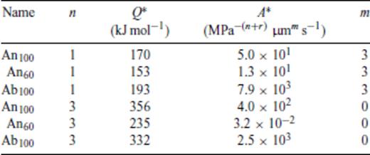
Creep parameters for plagioclase feldspars (from Rybacki & Dresen 2004).

Open in new tabDownload slide

In Fig. 6(a) we show the effect of composition in the ‘diffusion’ creep regime (d = 100 μm) for low (40 mW m⁻²), average (60 mW m⁻²) and high (80 mW m⁻²) heatflow. As with the computation of the geotherms (Section 2.1), we use assumptions on the thickness of the crust for different heatflow values, that is, 50 km for low, 40 km for average and 30 km for high heatflow. The effect of composition is not very large, although albite (Ab₁₀₀) is somewhat weaker than labradorite (An₆₀) and anorthite (An₁₀₀). For low heatflow, the viscosity of the lower crust is larger than about 3 × 10²⁰ Pa s, and for a channel of 10 km thickness, the viscosity is about 10²² Pa s. This indicates that deformation on glacial timescales is small, as a viscosity of 10²² Pa s corresponds for the crust (μ = 27 GPa, Table 4) to a Maxwell time of 10 kyr. However, if the assumption of lower crust consisting largely of plagioclase feldspars is true for cratonic areas, it shows that ductile deformation is also possible for cold areas as the Baltic Shield. For high heatflow, the viscosity of the lower crust decreases to 10¹⁷–10¹⁸ Pa s, although a reasonable channel is only formed for viscosities higher than about 10¹⁹ Pa s. For small grain size (d = 10 μm for the crust) viscosities become smaller than 10¹⁷ Pa s (see Fig. 6b, for labradorite) and are probably only realistic for localized shear zones. For large grain size (1000 μm) the lower crust becomes effectively elastic, but for this grain size, dislocation creep might be the dominant mechanism (e.g. Rybacki & Dresen 2004).

Figure 6.

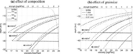
Viscosity estimates for ‘diffusion’ creep for different composition (d = 100 μm, a) and grain size (An₆₀, b). We use assumptions on the thickness of the crust for different heatflow values, 50 km for low, 40 km for average and 30 km for high heatflow. On the upper axis, we have also shown the strength for a strain rate of 3 × 10⁻¹⁸ s⁻¹. The brittle curves are computed from eq. (17) and the temperature profiles used are from Fig. 2(b).

Open in new tabDownload slide

In Fig. 7(a), we show the effect of composition on the viscosity and strength in the ‘dislocation’ creep regime for a strain rate of 3 × 10⁻¹⁸ s⁻¹. The effect of composition is somewhat larger than for diffusion creep, especially in the thickness of the channels, though for this strain rate there is low viscosity. For high strain rates (3 × 10⁻¹⁵ s⁻¹), viscosities decrease drastically (Fig. 7b, for labradorite), although viscosities are still larger than for diffusion creep with average grain size.

Figure 7.

Viscosity estimates for ‘dislocation’ creep for different composition (, a) and strain rates (An₆₀, b). The brittle curves are computed from eq. (17) and the temperature profiles used are from Fig. 2(b).

Open in new tabDownload slide

We conclude that albite is generally the weakest composition and anorthite, the strongest. Low-viscosity (∼10¹⁹ Pa s) is only reached in the diffusion creep regime for average grain size. For realistic perturbations (Section 4), we use albite in the diffusion creep regime, with average grain size as a reference, and use anorthite to test the sensitivity to composition. To test the sensitivity to grain size, we use albite with large grain size, as viscosities for small grain size seem to be not realistic. We use albite in the dislocation creep regime to test the sensitivity to creep regime.

4 Predictions for Northern Europe

In this section, we show the effect of the creep regime in the shallow upper mantle and composition and creep regime in the crust on predictions for Northern Europe. As a loading history, we use the RSES ice-load history (Lambeck et al. 1998) for the British Isles, Scandinavia and the Barents Sea, which is given from 30 kyr BP to present and of which we have plotted the ice heights at the last glacial maximum (LGM, 21 kyr BP) in Fig. 8(a). We add a 90 kyr linear glaciation phase (from 120 to 30 kyr BP), and we complement the ice-load history with a eustatic, that is, a geographically constant and meltwater equivalent, ocean-load history (e.g. Schotman et al. 2008), which has a maximum of about −130 m at LGM.

Total GIA-induced geoid heights at present, predicted from the laterally homogeneous model STD (RSES ice-load history, Fig. 9a) show a deep low of −4 to −5 m in the Gulf of Bothnia and bulge areas from 1000 km of the centre of loading outward. Note that to compare this with global predictions of GIA, the low harmonics (up to about degree 10) have to be filtered out to remove the effect of the former Laurentide ice sheet. We show the sensitivity to the ice-load history using the ICE-5G ice-load history (Peltier 2004), for which we have plotted the differences with the RSES ice heights at LGM in Fig. 8(b). The differences are especially large off the coast of Scotland and Norway and in the Barents Sea, where the ICE-5G model defines substantially larger ice masses. Geoid height ‘perturbations’ STDi-STD, that is, differences between predictions using ICE-5G and RSES and the same earth model, are given in Fig. 9(b). Note that for perturbations we use ‘centimetres’ as a unit because, especially for crustal perturbations (Section 4.2), amplitudes are not larger than tens of centimetres. The perturbations STDi-STD show a deep low over the Barents Sea, of a few metre. As the surface heatflow in the Barents Sea is relatively high (Fig. 3a), we expect crustal and asthenospheric low-viscosity in this area. In the presence of a weak lower crust or asthenosphere, we expect that the large differences in assumed ice mass will then lead in the following sections to relatively large differences in perturbations in this area.

Figure 9.

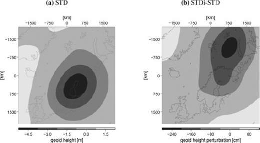
Total geoid heights as predicted by the laterally homogeneous earth model STD (RSES ice-load history, a) and geoid height height perturbations due to different ice-load histories (b). Perturbations are computed by subtracting predictions generated with RSES from predictions generated with ICE-5G (STDi-STD).

Open in new tabDownload slide

In Sections 4.1 and 4.2, we use creep laws for the shallow upper mantle (models DIF and DIS, Table 5) and crust (Table 6). As these creep laws are temperature-dependent (Sections 3.2 and 3.3), we use the temperature profiles from Fig. 2(b). Lateral heterogeneities are introduced by the dependence of the temperature profile on the surface heatflow and the crustal thickness (see Section 2.1). We use three areas of surface heatflow (40, 60 and 80 mW m⁻², Fig. 3a), based on the database of Pollack et al. (1993) and the extension of Artemieva & Mooney (2001), and five areas of crustal thickness (10, 20, 30, 40 or 50 km, Fig. 3b), based on CRUST2.0.

Table 5.

Models of the shallow upper mantle.

Open in new tabDownload slide

Table 6.

Models of the lower crust.

Open in new tabDownload slide

4.1 Shallow upper-mantle perturbations

In Fig. 10(a), we show geoid height perturbations ALVZ-STD. Perturbations are the difference between modelled field quantities of a specific earth model (e.g. ALVZ) and of a background model (e.g. STD). The laterally homogeneous ALVZ has a constant linear viscosity of 10¹⁹ Pa s from a depth of 100 to 160 km depth, see Table 5. The background model STD contains the RSES ice-load history. The ALVZ tends to decrease the total geoid height, as predicted from STD (Fig. 9a). Because the pattern is very similar to the total geoid heights, we do not expect that GOCE can add information on the asthenosphere because it will be difficult to separate the total geoid height from the perturbations. The similarity in the spatial pattern indicates that the ALVZ shows the same ‘deep flow’ behaviour (e.g. Schotman et al. 2008; Cathles 1975, p. 43) as the deeper upper mantle. This is not generally true for an ALVZ, because for a stiffer upper mantle or weaker lower mantle, the ALVZ can show ‘channel flow’ behaviour (e.g. Schotman et al. 2008; Cathles 1975, p. 49). In the next section, we discuss the difference between the two when we compare the response of a CLVZ with an ALVZ. Perturbations DIS-STD (Fig. 10b), where model DIS has wet olivine in the dislocation creep regime from below the crust to a depth of 220 km (Table 5), show a broad similarity with perturbations ALVZ-STD (compare with Fig. 10a). Amplitudes are comparable, but the centre of the perturbative high has shifted somewhat to the area of relatively high heatflow southwest of the Baltic Shield (compare with Fig. 3a).

Figure 10.

Geoid height height perturbations for a laterally homogeneous ALVZ (a) and for model DIS (wet olivine in the dislocation creep regime, b). Both models are given in Table 4 and perturbations are the difference with predictions from background model STD as shown in Fig. 9(a).

Open in new tabDownload slide

In Fig. 11(a), we show perturbations DIF-STD, where model DIF has wet olivine in the diffusion creep regime with average grain size in the shallow mantle, see Table 5. Compared with perturbations DIS-STD (Fig. 10b), the central peak is somewhat flatter, but the pattern is, in general, the same. This quite distinctive pattern, in which the high shifts to the region of average heatflow, seems to be very sensitive to the shallow geotherm, which is confirmed in the next section by the occurrence of perturbative highs under the former ice load in areas with average heatflow (compare e.g. Figs 12a and b). This indicates that it is necessary to use in the future tighter constraints on the geotherms, for example, by using shallow mantle temperatures derived from seismic tomography models (e.g. Goes et al. 2000). The predictions are not only sensitive to lateral heterogeneities but also to the ice-load history. In Fig. 11(b), we show again the effect of diffusion creep in the shallow mantle but now using ice-load history ICE-5G (DIFi-STDi). We see some large differences, especially in the Barents Sea area, but also some features that seem to be quite robust to changes in the ice-load history. These features are useful to ‘detect’, rather than constrain, shallow low-viscosity regions, because these features are not dependent on some uncertainties in the models (in this case the ice-load history), which means that they can be expected with a larger certainty in the measured gravity field.

Figure 11.

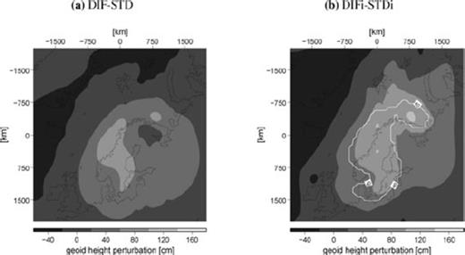
Geoid height perturbations due to diffusion creep in the shallow upper mantle for the RSES ice-load history (DIF-STD, a) and the ICE-5G ice-load history (DIFi-STDi, b). In (b), the area within the contour is robust to changes in the ice-load history with a standard deviation (of predictions DIF-STD and DIFi-STDi) smaller than 20 cm and a mean larger than 40 cm.

Open in new tabDownload slide

Figure 12.

Geoid height height perturbations due to a laterally homogeneous CLVZ (Table 4a) and for albite (Ab₁₀₀) in the diffusion creep regime (d = 100 μm) with DIS (Table 4) as a background model [ALB1(DIS), b]. Perturbations are the difference with (a) predictions from background model STD as shown in Fig. 9(a) (CLVZ-STD) and (b) predictions from background model DIS as shown in Fig. 10(b)[ALB1(DIS)-DIS].

Open in new tabDownload slide

These features we will call ‘spatial signatures’, which are, thus, geographical patterns that are associated with shallow low-viscosity regions that are only loosely constrained. To compare spatial patterns in two data sets, it is convenient to remove an off-set and scale factor. We estimate these from a least-squares fit of a test set of predictions to a reference set of predictions, which gives mostly a negligibly small offset and a scale-factor of 0.5–2. For the uncertainty in the ice-load history, for example, the least-square fit of the test set DIFi-STDi to the reference set DIF-STD gives a scale factor of 0.7. We then compute for each geographical location the mean and the standard deviation of the scaled perturbations (DIFi-STDi) and reference perturbations (DIF-STD). Those features that have a relatively small standard deviation are then robust to changes in the ice-load history. To only select those areas that have a distinct pattern, we choose a subset with a relatively large mean, which works well in most cases. The threshold levels are somewhat arbitrary, and for consistency with some examples further on, we take half a scale interval (in this case 20 cm) for the standard deviation and one scale interval (1/6 of the full scale, 40 cm) for the mean. In Fig. 11(b), the area within the contour labelled ‘40’ is therefore robust to changes in the ice-load history for perturbations due to diffusion creep in the shallow upper mantle with a standard deviation smaller than 20 cm and mean amplitudes larger than 40 cm.

4.2 Crustal perturbations

In Fig. 12(a), we show perturbations CLVZ-STD, where the laterally homogeneous CLVZ has a constant (i.e. temperature-independent), linear (in rheology) viscosity of 10¹⁹ Pa s from a depth of 20 to 30 km (see Table 6). Comparison with perturbations ALVZ-STD (Fig. 10a) shows mainly two things: due to the larger depth of the ALVZ compared with the CLVZ, the picture for an ALVZ is much smoother than for a CLVZ and an ALVZ ‘accelerates’ the process of GIA (e.g. smaller smaller geoid low under the load), whereas a CLVZ ‘delays’ the process (larger geoid low). The second difference is mainly due to the difference between deep flow for the ALVZ and channel flow for the CLVZ (Schotman & Vermeersen 2005; Cathles 1975, p. 219). If flow is constrained to a channel, first the channel at the edge of the load will relax, and due to very long relaxation of the low harmonics, the relaxation under the centre of the load will be delayed (Schotman et al. 2008; Cathles 1975, p. 158). For deep flow, the long wavelengths relax fastest, which results in a broad perturbation from under the load outward (Schotman & Vermeersen 2005; Cathles 1975, p. 219). Deep flow behaviour can be seen for the geoid height perturbations ALVZ-STD (Fig. 10a), which shows a broad perturbative high with a maximum of about 1.5 m under the load.

In Fig. 12(b), we show perturbations ALB1S-DIS. Model ALB1S has albite (Ab₁₀₀) in the diffusion creep regime (n = 1), with average grain size (d = 100 μm), see Table 6. Both the background model DIS and model ALB1S have wet olivine in the dislocation creep regime in the shallow upper mantle, see Tables 5 and 6, and both models are laterally heterogeneous. Amplitudes of geoid height perturbations ALB1S-DIS are comparable to perturbations CLVZ-STD, but the pattern of perturbations differs significantly, compare Figs 12(a) and (b). The low under the largest dome (around the Gulf of Bothnia), due to the long relaxation times induced by channel flow, is still visible, indicating that lower crustal flow seems to be possible in the Baltic Shield based on the adapted heatflow values and creep laws. The highs are now distributed around this low and occur mainly in areas south and west of the Baltic Shield that experienced significant loading and have average heatflow.

To show the sensitivity to the background model, we keep the same composition, creep regime and grain size in the crust, but change the background model from dislocation creep in the shallow upper mantle to diffusion creep in the shallow upper mantle (model ALB1F, see Table 6). If we compare the perturbations ALB1F-DIF (Fig. 13a) with the perturbations ALB1S-DIS (Fig. 12b), we see that the perturbations are very sensitive to changes in the background model as both figures show a significantly different spatial pattern, although with similar amplitudes. The perturbations are also sensitive to the ice-load history, which can be shown by comparing Figs 13(a) and (b). The latter is generated with ICE-5G (ALB1Fi-DIFi) and shows a somewhat different response in, for example, the Barents Sea area. In Fig. 13(b), we have also given contours for which the predictions are robust to changes in the ice-load history, with a threshold level for the standard deviation of 4 cm (half scale interval) and mean of 8 cm (one scale interval). As in Section 4.1, the contours are computed by scaling the test set (ALB1Fi-DIFi) to the reference set (ALB1F-DIF, scale factor: 0.6, see ‘ICE’ in Table 7) and computing for each geographical location the mean and standard deviation of the scaled test set and the reference set. Robust features are most likely to be recoverable from a high-resolution gravity field as, for example, expected from GOCE because they do not depend on certain assumptions, as in this case on the ice-load history.

Figure 13.

Geoid height perturbations for Ab₁₀₀ in the diffusion creep regime (d = 100 μm) with DIF (RSES ice-load history) as a background model [ALB1(DIF)-DIF, a] and DIFi [ICE-5G ice-load history] as a background model [ALB1(DIFi)-DIFi, b]. In (b), the area within the contour is robust to changes in the ice-load history with a standard deviation [of scaled test predictions ALB1(DIFi)-DIFi and reference predictions ALB1(DIF)-DIF] smaller than 4 cm and a mean larger than 8 cm.

Open in new tabDownload slide

Table 7.

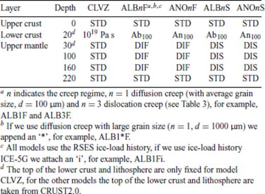
Model comparisons and data analysis.

Open in new tabDownload slide

In Fig. 14(a), we show perturbations ANO1F-DIF. ANO1F has a different composition of the lower crust (anorthite, An₁₀₀) than ALB1F (albite, Ab₁₀₀, see Table 6). Comparing with Fig. 13(a), we see that the pattern for this different composition is similar, although with smaller amplitudes, because An₁₀₀ is somewhat stronger than Ab₁₀₀ (Section 3.3). We have again indicated which areas are robust to changes in the composition by linearly fitting ANO1F-DIF to ALB1F-DIF (scale factor: 1.3, see ‘Composition’ in Table 7), which shows that the main lows and highs in the perturbations due to diffusion creep in the crust are robust to changes in composition. In Fig. 14(b), we show perturbations ALB3F-DIF. ALB3F has a different creep regime in the lower crust (dislocation creep, n = 3) than ALB1F (diffusion creep, n = 1), see Table 6. For these changes in creep regime (scale factor: 1.9, see ‘Regime’ in Table 7), only the highs seem to be robust (Fig. 14b), which implies that these highs are robust to both changes in composition and creep regime. As mentioned before, these features are most likely to be recoverable with GOCE, as these do not depend on composition nor creep regime in the crust.

Figure 14.

Geoid height perturbations for anorthite in the diffusion creep regime [d = 100 μm, An₁₀₀(DIF-DIF), a] and for albite in the dislocation creep regime [ALB3(DIF)-DIF, b]. Areas within contour lines are robust for changes in the composition (a) or creep regime (b) with a standard deviation smaller than 4 cm and a mean larger than 8 cm.

Open in new tabDownload slide

In the next section, we will test if GOCE can constrain the properties of the lower crust, that is, can discriminate between different compositions and creep regimes. From Fig. 14, we can already predict that it will be easier to discriminate between creep regimes than compositions, because the latter is more robust to changes in parameters. In the next section, we will also estimate if the conclusions depend on the background model (DIF versus DIS and DIFi).

5 Constraints from Future Goce Data

We expect GOCE to especially add information on the viscosity of the crust because of the high-resolution gravity field expected from GOCE and the distinct spatial patterns generated by crustal low-viscosity layers, as shown in the previous section. The latter is important to distinguish the signal due to low-viscosity layers from other signals due to, for example, thermally or chemically induced mass inhomogeneities in the crust. In the previous section, we have also shown which parts of the predictions are robust to changes in composition and creep regime of the lower crust and therefore facilitate the ‘detection’ of low-viscosity layers. Here we estimate the extent to which high-resolution gravity field information, as expected from GOCE, can ‘constrain’ the composition and creep regime of the lower crust. This involves the prediction of geoid height perturbations and testing which predictions have the best fit to the (synthetic) satellite gravity data. The data are able to constrain properties of the lower crust if they are able to distinguish between different predictions, that is, if there are significant differences in ‘prediction errors’. Here we will use the normalized prediction error (NPE, Hengl et al. 2004):

21

with p⁽¹⁾_i a ‘test’ prediction, d_i = p⁽⁰⁾_i+e_i synthetic data, with p⁽⁰⁾_i the reference prediction that generates the data, and e_i the errors. Both the test prediction p⁽¹⁾_i and the prediction p⁽⁰⁾_i that generates the synthetic data are perturbations. Hengl et al. (2004) take an NPE smaller than 40 per cent, in which (1 − 0.4²) × 100 ≈ 85 per cent or more of the variance of the data d is explained by a certain prediction p⁽¹⁾, as an acceptable prediction. For us, an acceptable test prediction p⁽¹⁾ is ‘not distinguishable’ from the synthetic data d, that is, from the reference prediction p⁽⁰⁾ in the presence of errors e. We take an NPE larger than 60 per cent, in which case 65 per cent or less of the variance is explained by the data, for a prediction that GOCE ‘can’ distinguish from the data.

We simulate the error introduced by the noise behaviour of the gradiometer onboard GOCE and downward continuation (recovery error) by adding random noise with a standard deviation of 1.5 mE (1 eötvös = 10⁻⁹ s⁻²) to 1 month of gravity gradients computed from a reference prediction p⁽⁰⁾ along a circular orbit (no polar gap) at 250 km altitude. For the reference prediction p⁽⁰⁾, we take perturbations due to a certain composition, creep regime and grain size of the lower crust (e.g. ANO1F-DIF, see Table 7). We recover the gravity field (i.e. geoid heights) from the gravity gradients using an iterative block-diagonal solution method, as described in Klees et al. (2000). The simulated error corresponds well with the expected GOCE performance computed from a more extensive simulation setup (Visser et al. 2002), as shown in Vermeersen & Schotman (2008). As a worst-case scenario, we also simulate the recovery error for a noise level of 3.0 mE. As explained in Section 1, we do not include any other error sources.

To obtain spectral information from our model, we use a 2-D FFT, as also used to compute geoid heights from the flat model (see Schotman et al. 2008). In Fig. 15(a), we have plotted the 2-D spectrum for the geoid height perturbations CLVZ-STD from Fig. 12(a). The wavenumbers k_x, k_y are defined as 2π/λ, with λ the wavelength in km corresponding to spatial scales (λ/2) = π/k. For comparison with the harmonic degree l, which is generally used in satellite gravity, we note that the spatial scale on the globe is defined as πR/l, that is, the harmonic degree l is equal to the normalized wavenumber Rk, with R the radius of the Earth (∼6378 km). The power spectral density (PSD) peaks for a wavenumber-distance from the centre of about 0.002–0.005 rad km⁻¹ (Rk∼ 12–32, spatial scales of ∼1500–600 km) and in a band between 0.01 and 0.015 rad km⁻¹ (Rk∼ 64–96, ∼300–200 km). This can be seen more clearly from a 1-D spectrum, in which the 2-D spectrum is radially averaged (i.e. we compute the total power in spherical bands and divide by the area of the band) and plotted as a function of wavenumber k_z (Fig. 15b). Next to the perturbations CLVZ-STD from the 2-D spectrum, we have plotted the spectrum of the recovery error for low (1.5 mE) and high (3.0 mE) noise level and the perturbations ALB1F-DIF, where ALB1F has albite (Ab₁₀₀) in the diffusion creep regime in the lower crust (see Fig. 13a for these perturbations in the spatial domain). We have also plotted in Fig. 15(b) the ‘sensitivity’ ANO1F-ALB1F to the composition of the lower crust and the sensitivity ALB3F-ALB1F to the creep regime, where the sensitivity is the difference between two sets of perturbations. We see that GOCE is sensitive to both composition and creep regime, though the sensitivity to composition seems to be low, which was already expected from Fig. 14(a), where we showed that the perturbations are quite robust to changes in composition. This is confirmed below when using the NPE to show the sensitivity of GOCE to composition and creep regime of the lower crust. We have applied a Bartlett window (e.g. Press et al. 1992, p. 547), which is a pyramid in 2-D, to the data, which surpresses a large part of the spectral leakage. This leakage is due to the inherent windowing of the data with a box when computing the 2-D Fourier-transform, which results in a convolution of the spectrum with a sinc-function, which is a sine-function divided by its argument (e.g. Press et al. 1992, p. 546). Some leakage is, however, still visible for low wavenumbers (<0.005 rad km⁻¹, Rk < 32) of the recovery error.

Figure 15.

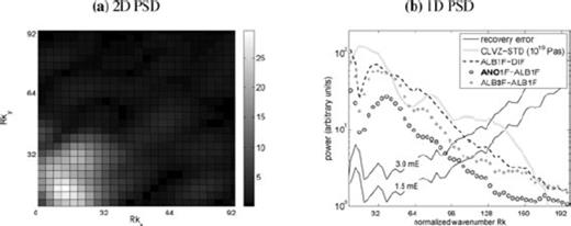
2-D power spectral density (PSD) of the perturbations due to a constant linear CLVZ as shown in Fig. 12a (CLVZ-STD, a) and the radially averaged 1-D PSD (b).

Open in new tabDownload slide

Before we can use the NPE to estimate to what extent GOCE can distinguish test predictions from the data, we first analyse the synthetic data. For this we can use the NPE, because for test predictions that are the same as the reference predictions that generated the synthetic data (p⁽¹⁾ = p⁽⁰⁾), the NPE gives (in per cent) the square root of the ratio of the power of the recovery error and the power of the data, that is, the square root of the noise-to-signal (N/S) ratio. For the data, we use perturbations ALB1F-DIF, which has a crust consisting of albite (Ab₁₀₀) in the diffusion creep regime, with a grain size of 100 μm. From Fig. 16(a), we see that the NPE for unfiltered data and predictions is quite high, which means that a considerable part of the variance of the data is due to noise. If we start filtering the data by removing the high wavenumbers (short wavelengths), the NPE drops to a minimum if we remove all wavenumbers larger than 0.015 rad km⁻¹ (Rk > 96). For 1.5 mE measurement noise, the NPE is about 33 per cent (N/S ratio of 0.1, see ‘REF’ in Table 7), which means that the recovery error contributes only 10 per cent to the variance of the data. For 3.0 mE, however, the NPE is close to 60 per cent (N/S ratio of 0.3, see ‘REF’ in Table 7), so that the error contributes almost 35 per cent to the data. From here on, we remove all wavenumbers larger than 0.015 rad km⁻¹ (Rk > 96).

Figure 16.

Effect of filtering on the NPE for REF [p⁽¹⁾ = p⁽⁰⁾ = ALB1(DIF), a] and the NPE for different test predictions p⁽¹⁾ with the data d = p⁽⁰⁾+e generated with p⁽⁰⁾ = ALB1(DIF) (b). For an explanation of ‘REF’, ‘COM’, ‘REG’, ‘GRA’, ‘AST’ and ‘ICE’, see Table 5.

Open in new tabDownload slide

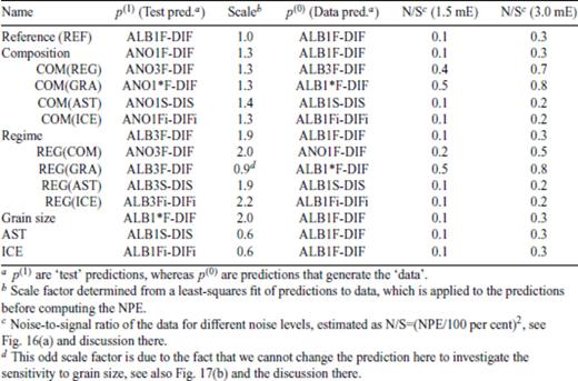
We now investigate if the correct prediction (‘REF’) has the smallest NPE for all noise levels and if other predictions can be distinguished from the data. To do this, we compute NPEs for different composition of the lower crust (anorthite, model ANO1F, ‘COM’ in Table 7), different creep regime (dislocation creep, model ALB3F, ‘REG’ in Table 7) and different grain size (1000 μm, model to ALB1*F, ‘GRA’ in Table 7). We also vary the background model, either the creep regime of the asthenosphere (to dislocation creep, model ALB1S, ‘AST’ in Table 7) or the ice-load history (to ICE-5G, model ALB1Fi, ‘ICE’ in Table 7). From Fig. 16(b), we see that the correct predictions always give the smallest NPE, also for high measurement noise level (3.0 mE). The NPEs for ‘COM’ are, however, close to the NPEs for ‘REF’, which indicates that GOCE can probably not discriminate between the two compositions. This was already expected from the 1-D PSD, where the sensitivity to composition was only slightly above the noise level (see Fig. 15b). All other predictions have NPEs larger than 60 per cent, which means that GOCE can discriminate between creep regime in the lower crust (‘REG’) and grain size (‘GRA’).

For changes in the background model-dislocation creep in the shallow upper mantle (‘AST’) or the ICE-5G load history (‘ICE’), an NPE larger than 60 per cent merely shows that-in the presence of albite in the lower crust, GOCE is predicted to be sensitive to both the creep regime in the shallow upper mantle and the ice-load history. However, an NPE larger than 60 per cent also shows that if we want to constrain properties of the crust, a priori information on the background model is needed because we will not predict the correct answer with a sufficiently small NPE, that is, a NPE smaller than 60 per cent. Because the influence of the recovery error is small, we can conclude that the difference in test and reference predictions is dominating, which is confirmed by the relatively low N/S ratios for ALB1F-DIF (Table 7). The increase of the NPE for increasing noise level, moreover, shows that there is a correlation between the predictions and the data, and that the NPEs are not generated by chance.

It is of course important to know if the conclusions we have drawn from Fig. 16(b) also hold for other synthetic data. Is GOCE, for example, also sensitive to the background model for dislocation creep or anorthite in the crust? Yes, also for dislocation creep regime or anorthite in the crust, GOCE is sensitive to the background model. But is it, for example, also true that GOCE cannot discriminate between albite and anorthite in the crust for other assumptions on the crust (creep regime, grain size) or background model (creep regime upper mantle, ice-load history)? We test this by computing NPEs for Ab₁₀₀ and An₁₀₀ in the crust for different assumptions on creep regime and grain size in the crust and different background models (Fig. 17a). Note that we now change, for each test, both the test prediction p⁽¹⁾ and the reference prediction p⁽⁰⁾ that generates the synthetic data, see from ‘COM(REG)’ to ‘COM(ICE)’ in Table 7. In the presence of error sources (‘1.5 mE’, ‘3.0 mE’), the conclusion that GOCE cannot discriminate between composition of the crust seems only to hold for changes in the background models [to DIS, ‘COM(AST)’ and DIFi, ‘COM(ICE)’], because for changes in the creep regime [‘COM(REG)’] or grain size [‘COM(GRA)’] of the crust, the NPE increases to about 80 per cent. The strong sensitivity of the NPE to the measurement noise indicates that the N/S ratio, as shown for ‘REF’ in Fig. 16(a), is large for both dislocation creep and large grain size in the crust (see Table 7). This means that the data for ‘COM(REG)’ and ‘COM(GRA)’ is largely controlled by the recovery error, and that the correct prediction is not acceptable (NPE larger than 60 per cent).

Figure 17.

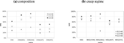
NPE for changes in composition (a) and in creep regime (b).

Open in new tabDownload slide

To see if the conclusion that GOCE can discriminate between diffusion creep and dislocation creep in the crust is robust, we change the composition [‘REG(COM)’] and grain size [‘REG(GRA)’] of the crust and the background model [to DIS, ‘REG(AST)’ and DIFi, ‘REG(ICE)’, see Fig. 17b). For a different composition of the crust [‘REG(COM)’], GOCE can still discriminate between diffusion and dislocation creep, but for different grain size [‘REG(GRA)’], the strong sensitivity of the NPE to the measurement noise indicates that the data is controlled by the recovery error (see Table 7), and that, if the crust shows diffusion creep with large grain size, GOCE measurements merely show noise. Note that the scale factor for ‘REG(GRA)’ is substantially different from the other scale factors of this figure, which is because we cannot change the grain size of the prediction, as it is in the dislocation creep regime. For ‘REG(AST)’ and ‘REG(ICE)’, the NPEs are smaller, indicating that it will be more difficult to discriminate between creep regime in the crust if the background model shows dislocation creep in the shallow upper mantle (model DIS) or if the ice-load history is ICE-5G (model DIFi).

6 Conclusions

Using a thermomechanical model (Section 2), we have estimated effective viscosities for plagioclase feldspars in the crust and olivine in the shallow (to a depth of 220 km) upper mantle (Section 3). For wet olivine in the diffusion creep regime with average grain size (8 mm), the viscosity at 200 km depth is 3 × 10²⁰ Pa s for low heatflow (40 mW m⁻²) and 6 × 10¹⁹ Pa s for average to high (60–80 mW m⁻²) heatflow. The lithospheric thickness for the process of GIA is 140 km for low heatflow and 60 km for average heatflow. The long-term (>1 Myr) thickness is smaller than 110 km for low heatflow and smaller than 30–40 km for average heatflow, depending on the strength of the lower crust. These values compare well GIA and effective elastic thickness studies for Northern Europe. For the crust, we use wet plagioclase feldspars, with albite, in general, the weakest and anorthite the strongest. Viscosities for average grain size (100 μm) and average to high heatflow can be as low as 10¹⁹ Pa s, and even for low heatflow, the lower crust seems to show some ductile behaviour.

We have shown the effect of creep laws on GIA-induced geoid height predictions in Northern Europe (Section 4) and have tested the sensitivity of future GOCE data to creep laws in the crust (Section 5). The main conclusions are:

• 1

  For a realistic load case, using the RSES ice-load history, amplitudes of perturbations due to diffusion or dislocation creep in the shallow upper mantle are comparable to a laterally homogeneous asthenospheric low-viscosity zone at a depth of 100 km, with a thickness of 60 km and a viscosity of 10¹⁹ Pa s. The spatial pattern is, however, more complicated, with the perturbative high shifting toward an area of average heatflow southwest of the centre of loading (see Fig. 10).

• 2

  Perturbations due to a weak lower crust are sensitive to the composition and creep regime of the crust, and the background model (diffusion or dislocation creep in the shallow upper mantle, ice-load history). The sensitivity to the background model is larger than to composition, but smaller than to creep regime.

• 3

  Some features of perturbations due to a weak lower crust are robust to changes in certain parameters (composition, creep regime, ice-load history). Robust features are features that differ less than 4 cm between a test and a reference prediction, and that have a relatively large amplitude (>8 cm). These features are most likely to be ‘detectable’ by GOCE. Some perturbative lows are for example robust to composition (e.g. the northern part of the Gulf of Bothnia) and some highs are robust to composition and to the creep regime (e.g. along the Norwegian coast), see Figs 14(a) and (b).

• 4

  Using normalized prediction errors (NPEs), we have shown that the synthetic data, consisting of a reference prediction and recovery errors as expected from GOCE, need to be filtered to minimize the noise-to-signal ratio. For different test predictions (changing the composition, grain size, creep regime or background model), the reference prediction always gives the lowest NPE, independent of the assumed measurement noise level.

• 5

  However, for a change in composition, the NPE is also small, which indicates that GOCE can probably not ‘constrain’ the composition of the lower crust, in contrast to creep regime and grain size.

• 6

  GOCE is also predicted to be sensitive to the background model in the presence of a crust consisting of plagioclase feldspars, irrespective of the creep regime. This also means if the wrong background model is assumed, we can no longer predict the correct properties of the lower crust, because prediction errors are larger than 60 per cent.

We plan to improve the constraints on the temperature profile in the Earth, using temperature at depth from seismic data (e.g. Goes et al. 2000), because the geoid height predictions are quite sensitive to the thermally induced lateral heterogeneities in our model. As the adapted ice-load history is contaminated by the assumed Earth stratification, we plan to couple our thermomechanical earth model to a thermomechanical ice sheet model (e.g. Bintanja et al. 2002) and estimate the ice-load history and Earth stratification at the same time. Finally, we have assumed in this study that the only error source in the GOCE data is the recovery error. However, especially, unmodelled shallow mass inhomogeneities are expected to mask gravity signals due to shallow low viscosity, and effective spatio-spectral filtering tools have to be developed to deal with this.

Acknowledgments

We are grateful to Cindy Ebinger, Volker Klemann and an anonymous reviewer for their valuable comments, Irina Artemieva (Geological Institute, University of Copenhagen, Copenhagen) for providing thermal data sets and heatflow data for continental Europe, Marta Pérez-Gussinyé (Institute of Earth Sciences ‘Jaume Almera’, CSIC, Barcelona) for providing data sets of effective elastic thickness estimates of Northern Europe, Pieter Visser (DEOS, Delft University of Technology, Delft) for providing the software to estimate predicted recovery errors of GOCE, Kurt Lambeck (RSES, Australian National University, Canberra) for providing the RSES ice-load history and Radboud Koop (NIVR, Delft, previously at SRON, Utrecht) and Rob Govers (IVAU, Utrecht University, Utrecht) for discussions over the past few years, which have lead to this paper. The geographical plots in this paper have been generated with GMT (Wessel & Smith 1991).

References