Multifractal Omori law for earthquake triggering: new tests on the California, Japan and worldwide catalogues

Summary

1 Introduction

The popular concept of triggered seismicity reflects the growing consensus that earthquakes interact through a variety of fields (elastic strain, ductile and plastic strains, fluid flow, dynamic shaking and so on). This concept was first introduced from mechanical considerations, by looking at the correlations between the spatial stress change induced by a given event (generally referred to as a main shock), and the spatial location of the subsequent seismicity that appears to be temporally correlated with the main event (the so-called aftershocks, King et al. 1994; Stein 2003). Complementarily, purely statistical models have been introduced to take account of the fact that the main event is not the sole event to trigger some others, but that aftershocks may also trigger their own aftershocks and so on. Those models, of which the Epidemic Type of Aftershock Sequences (ETAS) model (Kagan & Knopoff 1981; Ogata 1988) is a standard representative with good explanatory power (Saichev & Sornette 2006a), unfold the cascading structure of earthquake sequences. This class of models show that real-looking seismic catalogues can be generated by using a parsimonious set of parameters specifying the Gutenberg–Richter distribution of magnitudes, the Omori–Utsu law for the time distribution of aftershocks and the productivity law of the average number of triggered events as a function of the magnitude of the triggering earthquake.

Very few efforts have been devoted to bridge these two approaches, so that a statistical mechanics of seismicity based on physical principles could be built (see Sornette 1991; Miltenberger et al. 1993; Carlson et al. 1994; Sornette et al. 1994; Ben-Zion & Rice 1995; Ben-Zion 1996; Rice & Ben-Zion 1996; Klein et al. 1997; Dahmen et al. 1998; Ben-Zion et al. 1999; Lyakhovsky et al. 2001; Zoller et al. 2004, for previous attempts). Dieterich (1994) has considered both the spatial complexity of stress increments due to a main event and one possible physical mechanism that may be the cause of the time-delay in the aftershock triggering, namely rate-and-state friction. Dieterich's model predicts that, neglecting interactions between triggered events, aftershocks sequences decay with time as t^−p with p≃ 1 independently of the main shock magnitude, a value which is often observed but only for sequences with a sufficiently large number of aftershocks triggered by large earthquakes, typically for main events of magnitude 6 or larger. Dieterich's model is able to take account of a complex stress history, but it has never been grafted onto a self-consistent epidemic model of seismicity, taking account of mechanical interactions between all events.

Recently, two of us (Ouillon & Sornette 2005; Sornette & Ouillon 2005) have proposed a simple physical model of self-consistent earthquake triggering, the Multifractal Stress-Activated (MSA) model, which takes into account the whole space-time history of stress fluctuations due to past earthquakes to predict future rates of seismic activity. This model assumes that rupture at any scale is a thermally activated process in which stress modifies the energy barriers. This formulation is compatible with all known models of earthquake nucleation (see Ouillon & Sornette 2005, for a review), and indeed contains the state-and-rate friction mechanism as a particular case. The ultimate prediction of this model is that any main event of magnitude M should be followed by a sequence of aftershocks which rate decays with time as an Omori-Utsu law with an exponent p varying linearly with M.

Ouillon & Sornette (2005) have tested the linear dependence of p on M on the SCEC catalogue over the period from 1932 to 2003. Using a superposed epoch procedure (see Section 3.1) to stack aftershocks series triggered by events within a given magnitude range, they found that the p-value increases with the magnitude M of the main event according to p(M) = a₀M+b₀ = a₀(M−M₀), where a₀ = 0.10, b₀ = 0.37, M₀ = −3.7. Performing the same analysis on synthetic catalogues generated by the ETAS model, for which p is by construction independent of M, did not show an increasing p(M), suggesting that the results obtained on the SCEC catalogue reveal a genuine multifractality which is not biased by the method of analysis.

Here, we reassess the parameters a₀ and b₀ for Southern California, using an updated and more recent version of the catalogue, and extend the analysis to other areas in the world (the worldwide Harvard CMT catalogue and the Japanese JMA catalogue), to put to test again the theory and to check whether the parameters a₀ and b₀ are universal or on the contrary vary systematically from one catalogue to the other, perhaps revealing meaningful physical differences between the seismicity of different regions. We use three different methodologies to estimate p-values. The first one is a generalization of the construction of binned approximations of stacked time-series that we used in Ouillon & Sornette (2005). Here, we also introduce a new method specifically designed to take account of the possible contamination of the singular signature of the Omori-Utsu law by a regular and non-stationary background rate contribution that may originate from several different origins described in Section 3.3. This new method is coined the Scaling Function Analysis (SFA), and borrows the key ideas of the wavelet transform of multifractal signals. We also introduce another new method to shortcut the problem of missing events in aftershock sequences. Its main idea is to monitor the magnitude of the largest events as a function of time in a triggered sequence. We show that this allows us to determine the p-value, provided we know the b-value of the Gutenberg-Richter law (see Section 3.4).

Before focusing on the new statistical techniques for analysing aftershock sequences and presenting the results, we first recall the main concepts defining the MSA model. All analytical calculations have already been presented and detailed in Ouillon & Sornette (2005) and won't be repeated here. Only the relevant results will be used to compare with the empirical analysis.

In the last section of this paper, our results and theory will be discussed and confronted to recent models and ideas mostly published since Ouillon & Sornette (2005). We will in particularly show that most of them display data that are compatible with our observations (Peng et al. 2007), or present models that are special cases of ours (Helmstetter & Shaw 2006; Marsan 2006). Discrepancies with other works will be shown to be due either to declustering techniques incompatible with what we know about earthquake nucleation processes (Zhuang et al. 2004; Marsan & Lengliné 2008), or with physical models of fundamental different nature (Ziv & Rubin 2003).

2 The Multifractal Stress-Activation Model

2.1 Motivation and background

Mechanical models that try to predict the aftershock sequence characteristics from the properties of the main shock rupture are generally based on the spatial correlations between the Coulomb stress transferred from the main event to the surrounding space and the location of aftershocks. As the rupture characteristics of most of the aftershocks are unknown, and that many such events are even likely to be missing in the catalogues, the stress fluctuations due to aftershocks are neglected. While this approach aims at predicting the space-time organization of hundreds to thousands of aftershocks, it remains fundamentally a ‘one-body’ approach. Computing the stress transfer pattern resulting from the sole main shock and postulating that earthquake nucleation is activated by static stress (through mechanisms like rate-and-state friction or stress corrosion), one can predict the time dependence of the aftershocks nucleation rate which behaves as an Omori-Utsu law with exponent p≃ 1, independent of the magnitude M of the main event (Dieterich 1994).

Early works on stress transfer (see for example, King et al. 1994) have shown that some large recent earthquakes, like the Landers event, have certainly been triggered by a sequence of previous large events. Actually, there is a priori no support for the claim that the Landers event could have been triggered solely by large, well-defined previous events. Indeed, many other smaller events, for which rupture parameters are unknown, are likely to have played a significant role in the nucleation of that main shock (see also Felzer et al. 2002, for a similar discussion on the 1999 Hector Mine earthquake). This hypothesis is supported by the recent growing recognition that small earthquakes taken as a whole are probably as important as or even more influential in triggering future (small and) large earthquakes (Helmstetter et al. 2005).

We thus clearly need a ‘many-body’ approach to deal with the general problem of earthquake triggering, as any event, including aftershocks, is the result of a previous, complex space-time history of the stress or strain field, most of it being beyond our observation and quantification abilities. The MSA model has been developed to combine the complex stress history with the idea that events are activated by static stress. One specific prediction has been derived from a theoretical analysis of the model, namely the time dependence of the aftershocks rate and the most probable p-value that should be observed.

2.2 Description of the main ingredients of the MSA model

The MSA model is rooted in the general thermodynamic principle, that every earthquake results from a nucleation operating via thermally activated processes driven by stress. The justification of this assumption, as well as its relationship with all known earthquake nucleation mechanisms, is detailed in Ouillon & Sornette (2005). Thermal activation refers to the process in which a system in a state of energy E(t) at time t can reach a state of lower energy (the incipient rupture or frictional sliding state) via a jump over an energy barrier E₀ > E(t). The jump rate λ(t) is given by the Arrhenius law

1

where λ₀ is the background transition rate, T is the temperature and k is the Boltzmann constant. Such an Arrhenius law (1) is usually valid to describe transitions between atomic or molecular states. However, it is possible to show that expression (1) also describes the transition rates between macroscopic states, especially for the nucleation of macroscopic rupture, when allowing for a renormalization of the temperature into an effective ‘disorder’ temperature which is much larger than the thermodynamic temperature. Among others, Ciliberto et al. (2001) and Saichev & Sornette (2005) have shown that the presence of frozen heterogeneities, always present in rocks and in the crust, has the effect of amplifying the temperature of the rupture activation processes through the cascade of microdamage to the macrorupture, while conserving the same Arrhenius structure for the activation process. This renormalized temperature is then an effective temperature. In this formalism, the stress σ appears via the empirically established linear dependence of the energy barrier E₀−E(t) with σ (Zhurkov 1965) or equivalently expressing the energy term as a linear function of stress, which transforms (1) into

2

In this expression, σ(t) is the applied stress, σ₀ is the absolute height of the stress barrier (i.e. the material strength) and V is the activation volume, which is the volume of matter that collectively jumps over the barrier. This formulation of the nucleation rate is fully compatible with geomechanical concepts such as rate-and-state friction or stress corrosion, as shown in Ouillon & Sornette (2005). Lockner (1998) has also shown that the Arrhenius form, including both a stress and strain component in the energy, provides a good constitutive law for the brittle deformation of intact Westerly granite.

One may argue that the thermal dependency of a process such as rate-and-state friction holds only at the microscopic scale, depicting asperity creep. Anyway, the exponential dependency of the seismicity rate on the applied stress is still conserved at larger scales (see Dieterich 1994, for example, yet in that case one has to neglect the time dependency as it doesn't take account of multiple interactions and triggering). Indeed, most theoretical and experimental works on rate-and-state friction generally agree on the conclusion that the rate dependence of friction reflects the role of thermally activated physical processes at points of contacts between the sliding surfaces. This processes occur at microscopic scales, but renormalize at the macroscopic scale so that the parameters of the rate-and-state friction law depend on temperature. For example, Chester & Higgs (1992) studied experimentally the temperature dependence of parameters A and A−B as well as of the base friction coefficient μ₀ of the rate-and-state friction law for wet or dry ultrafine grained quartz gouge. In the velocity weakening regime (which is the regime for which earthquakes can occur, and that we implicitly assume to hold in our MSA model), they observed that an increase in temperature induces a decrease of A−B, so that the system is more unstable. This effect is enhanced in the wet case, while the value of A doesn't depend significantly on temperature. On the other hand, they also observe that, still in the velocity weakening regime, the base frictional strength increases with temperature for wet and dry tests, which agrees well with other experiments published by Blanpied et al. (1991) on granite gouge at hydrothermal conditions. Chester & Higgs (1992) and Chester (1994) propose an empirical modification of the rate-and-state friction law which takes account explicitly of the temperature and which predicts that changes in temperature and slip rate have opposite effects on the steady-state friction coefficient. At temperatures corresponding to seismogenic depths (i.e. from ≃ 300 to ≃ 600 K) the increase of the base friction is less than 5 per cent (Chester & Higgs 1992) while the change of A−B is much larger. All in all, we thus expect that the time to unstable slip of a given fault will be reduced when temperature increases, thus supporting our model in terms of a thermally activated seismicity rate. For other experiments and models of thermally activated friction processes see Ben-Zion (2003), Heslot et al. (1994) or Baumberger et al. (1999), among others.

At any location and time t, the earthquake nucleation rate is therefore

3

where λ′₀ absorbs both λ₀ and the exponential dependence on the stress barrier (which is assumed to be constant in space and time). For simplicity, the time and space dependent stress is assumed to be a scalar quantity, such as the Coulomb stress or any combination of the components of the full stress tensor.

The next step consists in writing down the definition of which reads

4

The first term in the right-hand side of this equation is the stress component due to the far-field tectonic loading. We assume that it can depend on space ( is the spatial location at which the earthquake rate is observed) but is constant with time. The second term is a double integral over the whole space and over all past times up to the present observation time t. The first term in this integral, is the number of events that occurred in an elementary space-time hypervolume . The next term, , is the stress fluctuation that occurred at the source of a past event located at spatial coordinate and time τ. The last term, , is the Green's function (possibly non-isotropic) that mediates this stress fluctuation from the source to the observation location and time.

Starting from the basic eq. (3) of thermal activation driven by stress and the eq. (4) for the stress field evolution, we now state several hypotheses that are needed in order to describe the statistics of earthquake triggering taking account of all past events whatever their time of occurrence, location and size.

Hypothesis 1: Every shock is activated according to the rate determined by Arrhenius law, function both of (possibly effective) temperature and stress.

Hypothesis 2: Every shock of magnitude M triggers instantaneously of the order of 10^qM events, which is equivalent of the productivity law in the ETAS model grounded on empirical observations (Helmstetter 2003). This hypothesis is discussed at the end of this paper.

Hypothesis 3: A separation of variables allows us to express the Green's function as

5

providing convenient simplifications in the theoretical analysis.

Hypothesis 4: the instantaneous stress fluctuations at any location due to the occurrence of seismic events depend on their spatial location , their rupture geometry and the spatial dependence of the Green's function. As most of these parameters are at best poorly known, and given the fact that a significant number of events are not even recorded at all (Sornette & Werner 2005), we follow Kagan (2004) and consider that the stress fluctuations are realizations of a random variable σ_fluc that may be positive or negative. We assume that the probability density function of this random variable can be written as

6

where σ_* is a small cut-off that prevents divergence of the pdf when σ_fluc = 0, while μ is an exponent which depends on and encapsulates the spatial structure of the fault pattern (where events occur), the Gutenberg-Richter law and the distribution of focal mechanisms (i.e. the rupture geometry) as well as f(r) (defined in eq. 5). The exponent μ thus encodes the entire spatial complexity of the problem.

Hypothesis 5: The behaviour of rock deformation is described by an elastoviscoplastic rheology. This means that the temporal part of the Green's function (5) can be written in a general way as

7

where h₀ is a scaling parameter, t_* is a small timescale that regularizes the power-law divergence at t = 0 and τ_M is the Maxwell time. We will suppose that it is larger than the timescale of observations (which is given in our case by the time interval over which aftershocks are thought to occur), so that τ_M≫t. It is important to understand that h(t) is indeed a renormalized function that encapsulates many stress relaxation phenomena like dislocations motion, pressure-dissolution or undetected earthquakes. The exponent θ thus encodes the entire temporal complexity of stress relaxation in the crust.

Taking account of all those hypotheses, we can rewrite the time evolution of the earthquake nucleation rate in a discrete form after spatial averaging (see Ouillon & Sornette 2005, for details)

8

which simply states that the present nucleation rate depends on past stress fluctuations (considered as random) occurring at times t_i, mediated to the present time t by the memory function h. We thus observe that the seismicity rate λ takes the form of an average seismicity rate λ_tec, modulated by a time-varying activation term. The formulation is thus non-linear. Note that, as the stress fluctuations σ_fluc can be positive or negative, they increase the seismicity rate in the former case, and decrease it in the latter case.

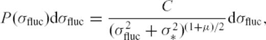
2.3 Main prediction of the MSA model

As the nucleation rate λ(t) obviously depends on the past seismicity rate (which controls the occurrence time t_i of past events), eq. (8) must be solved self-consistently. The mathematical framework necessary to solve this equation has already been presented in Ouillon & Sornette (2005), so we won't detail it here again. The final result is that, if the condition μ(1 +θ) = 1 is fulfilled, then

• (i)

  A magnitude M event will be followed by a sequence of aftershocks which takes the form of an Omori-Utsu law with exponent p.

• (ii)

  This exponent p depends linearly on the magnitude M of the main event.

• (iii)

  There exists a lower magnitude cut-off M₀ for main shocks below which they do not trigger (considering that triggering implies a positive value of p).

Our estimates below suggest that, for the Earth crust, μ(1 +θ) should lie somewhere within [0.73;1.5], thus bracketing the criterion for multifractality to hold. Ouillon & Sornette (2005) have shown that multifractality (and the main p(M) prediction discussed in this paper) also holds for a rather large set of values of μ and θ such that μ(1 +θ) = 1 is only approximately fulfilled. Saichev & Sornette (2006b) have identified that this stems from a generic approximate multifractality for processes defined with rates proportional to an exponential of a long-memory process [i.e. with power-law memory kernel such as our h(t) given by (7) for t < τ_M].

This model thus predicts that the exponent of the power-law relaxation rate of aftershocks increases with the size of the energy fluctuation, which is indeed the hallmark of multifractality (see for instance, Sornette 2006, for a definition and exposition of the properties associated with multifractality). This model has thus been coined the ‘MSA’ model (as used in the remaining of this paper).

In contrast with the phenomenological statistical models of earthquake aftershocks such as the ETAS model, the MSA model is based on firm mechanical and thermodynamic principles. A fundamental idea is that it integrates the physics of non-linear nucleation processes such as rate and state friction or slow crack growth. It is not possible to relate the ETAS model (Kagan & Knopoff 1981; Ogata 1988) to physically based earthquake nucleation processes. The above exposition shows that the non-linearity of the nucleation process translates necessarily into a non-linearity of the activation rates: the cumulative nucleation rate due to successive triggering events is not additive as in the ETAS model, but multiplicative. Stresses indeed add up, but not seismicity rates (which depend exponentially on the cumulative stress). Only the MSA model is compatible with the rate-and-state friction or slow crack growth process. The MSA model also takes account of negative stress fluctuations, which tend to decrease the seismicity rate, whereas, in the ETAS model, the effect of every event is to promote seismicity everywhere in space.

2.4 Possible significance of the condition μ(1 +θ) ≈ 1 ensuring the multifractality of earthquake sequences

2.4.1 Conjecture on an endogenous self-organization

Using the previous analysis of Ouillon & Sornette (2005) and anticipating the results shown below, we here discuss the possible physical interpretation of the condition μ(1 +θ) ≈ 1 found from the analysis of the MSA model for multifractality in the Omori law to hold. This condition suggests a deep relation between, on one hand, the exponent μ embodying all the spatial complexity and self-organization of the fault pattern and, on the other hand, the exponent θ encoding the temporal self-organization via earthquakes of the fault pattern. Such relation between power-law exponents associated with space and time organization are usually found only in critical phenomena. A natural interpretation rests on the deep association between faults and earthquakes, the former supporting the later, and the later growing and organizing the former. Indeed, one of the main results of modern seismology is that earthquakes occur on pre-existing faults. The fault network geometry thus controls the spatial location of earthquakes. In return, earthquakes are the key actors for the maturation and growth of fault networks. Such feedback loops lead to self-organization. This chicken-and-egg feedback has been proposed to lead to a critical self-organization (Sornette et al. 1990; Sornette 1991). The relationship between the exponents μ and θ encoding the space and time complexity of interactions between earthquakes is reminiscent of a similar relationship proposed by Sornette & Virieux (1992) between short- and long-term deformation processes. By solving a non-linear strain diffusion equation featuring a power-law distributed noise term encoding the Gutenberg-Richter distribution of earthquake sizes, Sornette and Virieux found, via a self-consistent argument that strain is scale invariant, that the Gutenberg-Richter b-value is determined endogenously for the largest events to the value 3/2. This value has received some confirming evidence (Pacheco et al. 1996) but it is fair to say that the determination of the shape of the distribution of earthquake sizes for very large and extreme events is still much debated (see for instance, Pisarenko & Sornette 2004, and references therein). A theory allowing to fix the exponents μ and θ in a similar way is still lacking. The MSA model takes these two exponents as exogenous, while a more complete theory encompassing the self-organization of earthquakes and faults at all timescales should determine them endogenously.

Let us know discuss briefly what we know presently of their possible values, both from theoretical considerations and empirical studies.

2.4.2 What is known on the exponent μ

A theoretical approach showed that the stress distribution due to a uniform distribution of equal-sized defects in an elastic medium obeys the Cauchy law (Zolotarev & Strunin 1971; Zolotarev 1986), which corresponds to μ = 1. Restricting potential events to occur on a fractal set of dimension δ embedded in a 3-D space, Kagan (1994) predicts that μ = δ/3, so that the Cauchy law should be associated with the upper bound of possible μ-values. Kagan (1994) also provides a measure of μ using static elastic stress transfer calculations from moment tensor solutions of the worldwide Harvard CMT catalogue, which allow him to estimate stress increments due to past events at the locii of future events, as well as their statistical distribution. Using pointwise double-couple approximations of event sources, he observes that the large stress tail of the distribution (which mainly characterizes stresses transferred by nearby events) behaves as a power law with μ = 1, hence as a Cauchy law. As this value is the one that corresponds to a uniformly random distribution of sources, he proposes that this may be due to earthquake location uncertainties. Those uncertainties make earthquake clusters look spatially random at short spatial ranges, so that their fractal dimension δ is close to 3, and thus μ = 1. Considering the distribution of smaller stress increments, he obtains μ = 0.74. Such a value corresponds theoretically to δ = 2.2, in excellent agreement with the spatial correlation dimension of earthquake hypocentres (Kagan 1994). Marsan (2005) tried to estimate μ directly from a natural catalogue of events (Southern California). He computed the distribution of stress fluctuations taking account only of target sites that were the locii of future pending events. The stress value is computed by taking account of the focal mechanisms of the events. This approach yields a μ-value close to 0.5.

While it seems clear that the hypothesis that the distribution of source stresses is heavy tailed (power law) with a small exponent of the order of 1, all these works suffer from one or several problems.

• (i)

  These works neglect the fact that a huge majority of events occur without being recorded at all (the smallest magnitude events) and are thus excluded from the statistics.

• (ii)

  Some potential nucleation sites experienced stress fluctuations from past recorded events but didn't break during the instrumental period and are thus excluded from the statistics too.

• (iii)

  Marsan (2005) did not consider triggered events that occurred too close to the triggering event, so that he could use a pointwise source approximation. Using such simplified source geometries certainly influences the resulting value of μ, as the symmetry properties of the stress field are significantly altered in the vicinity of the fault.

• (iv)

  Moreover, the rupture pattern on the fault plane is generally quite complex, so that stress fluctuations occur on the rupture plane itself (and are thought to be the reason of the occurrence of the majority of aftershocks there). Those stress fluctuations are mediated in the surrounding medium by the Green's function, and are thus not taken into account by the studies cited above. It is thus certainly very difficult to assess a precise value of μ from a natural data set.

2.4.3 What is known on the exponentθ

Several different mechanisms of stress relaxation may contribute to the determination of the exponent θ.

A first mechanism involves linear viscous relaxation processes. If stress relaxation in the crust is assumed to be dominated by linear viscous processes, then stress relaxes with time as t^−3/2 in a 3-D medium (providing an appropriate description for stress fluctuations due to small earthquakes), and as t⁻¹ in a 2-D medium (that may apply for large events, that break throughout the brittle crust). If such a transition exists, then θ should vary from 1/2 to 0 for magnitudes, respectively, smaller and larger than about 6–6.5.

A second mechanism assumes that stress relaxation is only due to seismicity itself, as successive earthquakes occur to release stored stress. Suppose that at a given location , the initial applied stress is σ(t = 0). As earthquakes are thermally activated, the average waiting time for the first event to occur is given by eq. (2)

9

Once the first event occurred, the local stress drops by an amount Δσ that we consider to be a constant from event to event. The new applied stress is σ(t = t₁) = σ(t = 0) −Δσ. The average waiting time t₂ till the second event is also obtained using eq. (2), with σ(t) = σ(t₁). This yields . Iterating this reasoning, we can show that t_n, the average waiting time between events (n− 1) and n, is . As waiting times between successive events define a geometrical sequence with common ratio , the average seismicity rate at location decreases as 1/t. As the cumulative stress drop is proportional to the number of events, the stress relaxes with time as

10

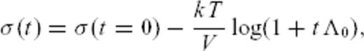
where Λ₀ depends on the thermal activation parameters, the stress drop and the initial stress. For timescale , expression (10) is undistinguishable from

11

thus yielding an estimate .

This model of stress relaxation has also a simple analytical solution in the case where the stress drop is just proportional to the applied stress. In that case, the stress drop associated with the first event is γσ(t = 0) for some coefficient 0 < γ < 1, so that σ(t₁) = (1 −γ)σ(t = 0). The stress drop during the second event is γσ(t₁), and so on. This leads to a differential equation of the form

12

so that time t can be solved as a function of σ

13

Stress first relaxes with time logarithmically (hence like a power law as shown from the transition from 10 to 11) at small times, and exponentially at large times, in agreement with the postulated form (7).

3 Methodology Of The Empirical Multifractal Analysis

3.1 Step 1: selection of aftershocks

In this paper, we use a method for stacking aftershock time-series which is slightly different from the one used in Ouillon & Sornette (2005), especially in the way we take account of the time dependence of the magnitude threshold M_c(t) of completeness of earthquake catalogues.

All earthquakes in the catalogue are considered successively as potential main shocks. For each event, we examine the seismicity following it over a period of T = 1 yr and within a distance R = 2L, where L is the rupture length of the main shock, which is determined empirically from the magnitude using Wells & Coppersmith (1994)'s relationship:

14

The same relationship is used for all catalogues in the absence of a more specific adaptation to the Japanese JMA catalogue. Concerning the Harvard CMT catalogue, it can be expected that a relationship relating magnitudes to rupture length would be a weighted mixture of different relationships holding in different parts of the world, with variations resulting from local tectonic properties. We will see below that the novel method we propose, the SFA, is actually devised to take account of the uncertainties resulting from the use of approximate length-magnitude relationships. If the radius R is smaller than the spatial location accuracy Δ (which is assumed here for simplicity in a first approach to be a constant for all events in a given catalogue), we set R = Δ. If an event has previously been tagged as an aftershock of a larger event, then it is removed from the list of potential main shocks, as its own aftershocks series could be contaminated by the influence of the previous, larger event. Even if an event has been removed from the list of main shocks, we look for its potential aftershocks and tag them as well if necessary (they are themselves excluded from the list of main shocks in the stacked time-series).

Aftershock time-series are then sorted according to the magnitude of the main event, and stacked using a superposed epoch procedure within given main shock magnitude ranges. This means that we shift the occurrence time of each main shock to t = 0. For each main event, the associated aftershock sequence is shifted in time by the same amount. In this new time frame, all events tagged as aftershocks in the original catalogue occur within the time interval [0;T]. We choose main shock magnitude intervals to vary by half-unit magnitude steps, such a magnitude step being probably a rough upper-bound for the magnitude uncertainties (see Werner & Sornette 2008, and references therein). Shifting of individual aftershock time-series to the same common origin allows us to build composite aftershock sequences that feature a large amount of events, even if the magnitude of the main shock is low. For example, a single magnitude 2.0 event may trigger at most 1 or 2 detected aftershocks (and most of the time none at all), which makes impossible to quantify any rate. But collecting and stacking 10 000 aftershock sequences triggered by as many magnitude 2.0 events allows one to build a time-series featuring several hundreds to thousands of aftershocks. An average p-value can then be estimated with a good accuracy for main shocks of such small magnitude ranges.

This methodology to build aftershocks stacked series is straightforward when the magnitude threshold M_c(t) of catalogue completeness is constant with time, which is the case for the Harvard catalogue, for example. For the SCEC and JMA catalogues, we take into account the variation of M_c(t) as follows. Individual aftershock times series are considered in the stack only if the magnitude of the main event, occurring at time t₀, is larger than M_c(t₀). If this main event obeys that criterion, only its aftershocks above M_c(t₀) are considered in the series. This methodology allows us to use the maximum amount of data with sufficient accuracy to build a single set of stacked time-series of aftershock decay rates. The time variation of M_c has been estimated by plotting the magnitude distribution of earthquakes year by year in each catalogue, and assuming that M_c coincides with the onset of the Gutenberg-Richter law.

The time variation of M_c we propose should not be considered too strictly. For example, if a catalogue is considered to be complete down to M_c = 3.0, this does not prevent it to be incomplete during the first days that follow a magnitude 7 event. Indeed, any declustering algorithm should first define a M_c(t) function that describes the detection threshold magnitude for isolated main shocks. But in return, estimating M_c(t) necessitates to decluster the catalogue first. As our estimation of M_c(t) takes account of all events in the catalogue, including aftershocks, it thus provides an overestimate of the M_c(t) threshold for main shocks.

Ouillon & Sornette (2005) used a slightly different strategy accounting for the variation of M_c with time by dividing the SCEC catalogue into subcatalogues covering different time intervals over which the catalogue was considered as complete above a given constant magnitude threshold. This led Ouillon & Sornette (2005) to analyse four such subcatalogues separately. The robustness of the results presented below in the presence of these algorithmic variations is a factor strengthening our belief that the multifractal time dependent Omori law that we report in this paper is a genuine phenomenon and not an artefact of the data analysis or of the catalogues.

The method we used to decluster our earthquake catalogues involves a certain amount of arbitrariness, like the choice of the sizes of the spatial and temporal windows to select aftershocks. The values we chose are similar to those used in other works using the same kind of declustering technique. We should mention that two techniques have been recently introduced to remove the arbitrariness of aftershock selection rules. Each of them assumes that each event has a given probability of being triggered by any of the events that preceded it, and a probability of being a spontaneous background event. All probabilities (that are equivalent to rates) sum up to 1 for each event. The first approach (Zhuang et al, 2004) assumes that the phenomenology of earthquakes space-time organization can be modelled by an ETAS process with energy, space and time power-law kernels. The declustering procedure just consists in inverting the parameters controlling the shapes of the kernels, like the p-value. This is done using a maximum likelihood approach. The second approach (Marsan and Lengliné, 2008) is a non-parametric one based on an expectation-maximization algorithm. In this case, the functional form of the kernels is a priori unknown and is inverted as well. This last approach is must more general than the one of Zhuang et al (2004) and has been claimed by its authors to be completely model-independent, and thus free of any arbitrariness. We would like to moderate this view and point out that this method is certainly the best one to use when one is dealing with a data set generated by an ETAS-like algorithm, but that it is not adapted to the declustering of earthquake catalogues. As previously mentioned, the method of Marsan and Lengliné (2008) assumes that at any place and any time, the earthquake nucleation rate is the sum of individual rates triggered by each of the events that occurred in the past, plus a background rate. This assumption has the advantage of allowing easy computations, but it is fundamentally incompatible with what is known about the physics of earthquakes. If we assume that stress is elastically redistributed after any event, then the stress at any place and time is the sum of previous stress redistributions (and far-field loading). If we assume that earthquakes are exponentially activated by stress and temperature, an assumption which is underlying most models of earthquake nucleation, then it follows that the resulting rate due to previous events is proportional to the product of individual triggered rates, not their sum. The approach of Zhuang et al. (2004) and Marsan & Lengliné (2008) is thus intrinsically incompatible with all we know about earthquake nucleation physics. Indeed, introducing this kind of linear declustering methodology assumes a priori that earthquakes are governed by a linear process, which is quite a strong assumption. The fact that Marsan & Lengliné (2008) observe a rather weak magnitude-dependent p-value is likely to be the consequence of such an a priori choice, since linear models do not predict magnitude-dependent p-values by construction. We are perfectly aware that our simple method of declustering separates some main shocks from the rest of seismicity, whereas our model states that earthquake triggering involves the whole hierarchy of triggering events, down to very small and even undetected magnitudes. Unfortunately, no general non-linear declustering scheme, taking account of the triggering effect of every event, presently exists. The main difficulty to define such a non-linear probabilistic model is that one has to know in advance the nature of the non-linearity (which in our case amounts to deal with elastic stresses and their sign).

3.2 Step 2: fitting procedure of the stacked time-series

Once aftershocks time-series have been selected, stacked, and sorted according to the main shock magnitude, we fit the binned data with the following law

15

which includes an Omori-like power-law term and a constant background rate B. Here, N(t) is the rate of triggered seismicity at time t after a main shock that occurred at t = 0. The time axis is binned in intervals according to a geometrical series so that the width of the time intervals grows exponentially with time. We then simply count the number of aftershocks contained within each bin, then divide this number by the linear size of the interval to obtain the rate N(t). This seismicity rate is fitted with an Ordinary Least-Squares (OLS) algorithm, the fitting parameters A, B, p being obtained by a standard grid search. It could be argued that the background term B should be constrained by estimating the mean seismicity rate prior to main shocks. We thus built the corresponding stacked time-series of events occurring before our selected main shocks (in the same time and space windows) and observed that they behaved as inverse Omori-Utsu laws, so that a constant background term B could not be estimated this way. The observation of such accelerating seismicity rates prior to events of any magnitude in stacked time-series has already been reported in Jones & Molnar (1979) and Helmstetter & Sornette (2003).

As the linear density of bins decreases as the inverse of time, each bin receives a weight proportional to time, balancing the weight of data points along the time axis. In our binning, the linear size of two consecutive intervals increases by a factor α > 1. Since the choice of α is arbitrary, it is important to check for the robustness of the results with respect to α. We thus performed fits on time-series binned with 20 different values of α, from α = 1.1 to 3 by step of 0.1. We then checked whether the fitted parameters A, B and p were stable as a function of α. We observed that the inverted parameters do not depend significantly on α. We used the 20 estimations of A, B and p for the 20 different α's to construct their averages and standard deviations. For some rare cases, we obtained p-values departing clearly from the average (generally for the largest or smallest values of α)-we thus excluded them to perform a new estimate of p, following here the standard procedure of robust statistical estimation (Rousseeuw & Leroy 1987). In order to provide reliable fits, we excluded the early times of the stacked series, where aftershock catalogues appear to be incomplete (Kagan 2004). Finally, an average p-value (and its uncertainty) determined within the main shock magnitude interval [M₁;M₂] is associated with the magnitude . Our approach extends that of Ouillon & Sornette (2005) who performed fits on the same kind of data using only a single value α = 1.2.

The time interval over which the fit is performed is chosen such that the event rate time-series scales as an Omori-Utsu law whatever the value of the α-parameter. For a given magnitude range, all time-series are thus fitted using the same time interval. In return, this ensures that the time interval over which a power-law scaling is observed does not depend on the choice of a unique and arbitrary α value. The end time is usually taken as t = 1 yr, except if a large burst of activity occurs near that time (as is the case for example for the largest magnitude range in Fig. 3). The beginning of the fitting interval has been chosen by eye inspection for each value of α and we subsequently checked that the chosen common fitting interval for the least-squares approach was similar to the one used for the SFA method (see below).

Figure 3.

Binned stacked series of aftershock sequences in the SCEC catalogue (after removing the events in the Brawley zone) for various magnitude ranges. Magnitude ranges are, from bottom to top: [1.5;2], [2;2.5], [2.5;3], [3;3.5], [3.5;4], [4;4.5], [4.5;5], [5;5.5], [5.5;6], [6;6.5], [6.5;7], [7;7.5], [7.5;8]. The solid lines show the fits to individual time-series with formula (15). All curves have been shifted along the vertical axis for the sake of clarity.

Open in new tabDownload slide

For each magnitude range, we thus have 20 different binned time-series corresponding to different values of α. For the sake of clarity, we only plot the binned aftershocks time-series whose p-value is the closest to the average p-value obtained over the 20 different values α for that magnitude range. Its fit using eq. (15) will be plotted as well.

Using binned time-series and OLS fits is very popular in the literature to determine p-values. The next two sections will point out that the quality of the selected aftershock time-series generally suffers from sampling biases. For low magnitude main shocks, the sequences can be contaminated by sequences triggered by previous events. Sequences triggered by large magnitude events often suffer from time-dependent undersampling of small aftershocks. The next two sections address those problems and propose new methods to solve them. They will also provide independent estimations of the p-values for the different main shock magnitude ranges.

3.3 Step 3: scaling function analysis

The method presented above to fit binned data uses a magnitude-dependent spatio-temporal window within which aftershocks are selected. Consider a main event E₁ whose linear rupture size is L. The present methodology assumes that any event located within a distance 2L of E₁, and occurring no more than 1 yr after it, is one of its aftershocks. Conversely, any event located at the same distance but which occurred after only just a little more than 1 yr after the main shock is not considered as its aftershock but as a potential main shock E₂, with its own aftershocks sequence which can be used for stacking. Actually, choosing such a sharp definition for the size of the time window to qualify aftershocks is quite arbitrary. No such choice will get rid of the possibility that the aftershocks sequence of an event E₂ may still be contaminated by the sequence triggered by the preceding event E₁, especially if M(E₁) > M(E₂). Since the formula of Wells & Coppersmith (1994) does not strictly apply to each event in a given catalogue, one can imagine many other scenarios of such a contamination that may also originate in the underestimation of L. A step towards taking into account this problem is to rewrite expression (15) for the time evolution of the sequence triggered by E₂ as

16

where B(t) is a non-stationary function that describes both the constant background seismicity rate and the decay of the sequence(s) triggered by E₁ (and possibly other events occurring prior to E₂). Here, t is the time elapsed since the event E₂ occurred, as we want to characterize the sequence which follows that event. As the event E₁ occurred before the event E₂, B(t) is not singular at t = 0. It is thus a regular contribution to N(t), which we expect to decay rather slowly, so that it can be approximated by a polynomial of low degree n_B. We thus rewrite eq. (16) as

17

where the sum on the right-hand side now stands for B(t). We have a priori no information on the precise value of n_B, nor on the values of the coefficients b_i. For n_B = 0, we recover the constant background term B of expression (15). On the other hand, n_B might be arbitrarily large in which case the coefficients b_i's can be expected to decrease sufficiently fast with the order i to ensure convergence, so that only the few first terms of the sum will contribute significantly to B(t). Their number will depend on the fluctuations of the seismicity rate at times prior to the event E₂. The effect of this polynomial trend is to slow down the apparent time decay of the aftershocks sequence triggered by event E₂, hence possibly leading to the determination of a spurious small p-value. This could be a candidate explanation (see the Appendix) for Ouillon & Sornette (2005)'s report of small values of p for main events with small magnitudes. One could argue that their stacked aftershocks time-series might be contaminated by the occurrence of previous, much larger events (as well as of previous, smaller but numerous events).

In order to address this question, that is, to take account of the possible time-dependence of B, two strategies are possible:

• (i)

  The 20 different binned time-series can be fitted using eq. (17) with the unknowns being A, p, n_B and the b_i's,

• (ii)

  One can use weights in the fitting procedure of the original data so that the polynomial trend is removed. One is then left with a simple determination of A and p alone.

We have implemented the second strategy in the form of what we refer to as the ‘SFA’. The Appendix describes in details this method that we have developed, inspired by the pioneering work of Bacry et al. (1993) on wavelet transforms, and presents several tests performed on synthetic time-series to illustrate its performance and the sensitivity of the results to the parameters. Those tests show that the SFA method will be very useful to process aftershock sequences triggered by small main shocks for which a power-law scaling can be observed down to very small timescales. For sequences following larger magnitude events, a breakdown of scaling properties is often observed due to magnitude-dependent sampling problems at early times. The help of the SFA method is then more limited (see the Appendix). The next section proposes still another new method that allows one to deal with those undersampling biases. Note that the SFA method indeed introduces another parameter n_D which controls the shape of the wavelet close to t = 0. The Appendix discusses the role of this parameter as well. In their attempt to quantify diffusion processes within individual aftershock sequences of large Californian events, Helmstetter et al. (2003) performed a wavelet analysis of triggered time-series at various spatial scales. This wavelet analysis in the time domain is indeed equivalent to the present SFA in the case n_B = n_D = 0.

3.4 Step 4: time variation of maximum magnitudes

Fitting of binned time-series or of the SFA coefficient as a function of timescale requires in both case to select reliable aftershock catalogues. This step is by far the most difficult, especially for short timescales after a large event, as the earthquake activation rate is so large that it proves impossible to pick up seismic waves arrival times and locate every event, especially the smallest ones. This human and instrumental limitation is generally invoked to explain the observed roll-off of aftershocks nucleation rate just after a large main shock.

It is generally assumed that this sampling bias can be mathematically expressed by a time-varying aftershock detection magnitude threshold, above which the aftershock catalogue is considered as complete, and below which it is considered as incomplete. For example, a detailed analysis of aftershock sequences in Southern California led Helmstetter et al. (2005) to propose that this threshold varies as

18

where M is the magnitude of the main event, and t is the time elapsed since that event in days. For example, if M = 4.5, this means that the aftershock catalogue is complete above magnitude m_th = 2 for times larger than 3 min. This time reaches about 3 weeks if M = 7.5.

Helmstetter et al. (2005) use eq. (18) to correct their aftershock time sequences for the missing events using a very simple reasoning: if a main shock of magnitude M occurs at time τ = 0 then, at time t, the catalogue of aftershocks is complete above a magnitude m_th given by eq. (18). Assuming that the Gutenberg-Richter law holds at any time with a constant b-value, it follows that N₀(t), the theoretical total number of events triggered at time t, is proportional to , where N_obs[m > m_th(M, t)] is the observed number of aftershocks of magnitude larger than m_th(M, t). Plotting N₀(t) as a function of t thus allows one to estimate the rate of aftershocks as a function of time, including missing events in the time-series. Helmstetter et al. (2005) observe that this approach provides a significant increase of the temporal range available to measure the p-value of the Omori law.

While this approach seems at first sight simple and efficient, it nevertheless possesses several drawbacks. First, it necessitates to carefully analyse several aftershock sequences to obtain eq. (18), which is a very tedious task. It is also obvious that all coefficients in this equation will depend on the geometry of the permanent seismic stations network at the time of occurrence of the main event. Thus, this equation cannot be used for all earthquakes in a given catalogue: every time a change occurs in the geometry of the seismograph network, coefficients in eq. (18) have to be updated, requiring a new analysis of a sufficient number of individual sequences spanning a large spectrum of main shock magnitudes. This also means that all coefficients have to be determined for a single given catalogue: the various parameters for Southern California are not valid for the JMA or the Harvard catalogues.

Another important problem is that m_th(M, t) has a much more complex time-dependence than the one given by eq. (18). To show this, we shall consider a simple example. We assume that a main event E₁ of magnitude M₁ = 7.5 occurs at time τ = 0. As mentioned above, using eq. (18) predicts that all triggered events of magnitude m > 2 will be detected after a time lapse of about 3 weeks. We now suppose that, 6 months after the main event, another event E₂ of magnitude M₂ = 7.5 occurs within a short distance of E₁. This event, as well as the majority of its aftershocks, will thus be considered as aftershocks of event E₁. It is now important to understand that, after event E₂ occurs, many events of magnitude m < 2 will be missed for a time span of about 3 weeks. It follows that the aftershock catalogue of event E₁ will also be depleted of the same quantity of aftershocks during a time interval that spans (6 months, 6 months + 3 weeks). The simple prediction of eq. (18) is thus not verified for event E₁. One can extend this simple reasoning to different values of M₁ and M₂ and show that, in an aftershock time sequence, every aftershock is itself followed by a time interval within which events are missing. It follows that any aftershock time sequence misses events not only at its beginning, but also all along its duration. It is a priori difficult to correct for this effect as it depends heavily on the specific time distribution of the aftershock magnitudes characterizing each sequence.

The new method we propose in this section allows one to analyse aftershock time-series without the need to define any magnitude detection threshold. It is based on two simple assumptions: the first one is that the Gutenberg-Richter law holds down to the smallest possible earthquake source magnitude M_min and that the b-value is independent of the magnitude of the main shock and of the time elapsed since that main shock occurred. The second assumption reflects the way seismologists deal with, select and process seismic signals: for a variety of reasons, one is mostly interested in the largest events in a time-series. This stems from the fact that they are generally associated with a high signal-to-noise ratio and are detected by a large number of stations, allowing a clean inversion of the data (such as hypocentre location, focal mechanism and source dynamics). They also dominate the rate of energy and moment release in the sequence, and thus the potential damage that may be due to large aftershocks. As much interest thus focuses on the largest events, and because they are obviously easier to detect, it is reasonable to state that, in any given time interval, the event that has the smallest probability to be missed is the largest one. Indeed, even if the P- and/or S-waves arrival times prove to be unreadable due to the superposition of waves radiated by numerous other smaller events, one will anyway be able to pick up the arrival times of the maximum amplitude of the P or S waves, which shall be sufficient to provide the spatial location of the associated event and compute its magnitude with reasonable accuracy. We will thus assume that this reasoning holds true even after the occurrence of a large event, except maybe during the early part of the associated coda waves, whose amplitude may completely hide any immediate aftershock.

We thus logarithmically bin the time axis to the right of the origin defined at the time of occurrence of a main event, by defining a set of discrete time interval boundaries t_i, i ≥ 0, with t_i+1 = αt_i, where α > 1 and t₀ a very small strictly positive arbitrary time. Assuming that the total nucleation rate of aftershocks behaves on average as N(t) = K t^−p, we can compute the total average number of events N_i occurring in time bin i (that runs from t_i to t_i+1):

19

which could be used to retrieve p if we were able to detect and locate all events down to M_min. As the Gutenberg-Richter law is assumed to hold over the whole magnitude range, the total average number of events in time bin i can also be written as where M_i is the magnitude of the largest event that occurred within that bin. This value for N_i just states that there is on average one event of magnitude M_i in the time bin i. Writing that

20

and using eq. (19) to express N_i and N_i+1, we obtain

21

which is an arithmetic progression with common difference . If we now set M_max(t_i) = M_i, we get M_max(t_i) = m₀+iρ, where m₀ is a constant. Noting that t_i = t₀αⁱ, we get , yielding finally

22

M_max(t_i) thus varies linearly with log ₁₀(t_i), with a slope . The slope is zero if p = 1: in that case, the total number of events remains constant within each logarithmic time bin, so that the typical maximum magnitude within each bin does not vary. The observation that the total number of events counted in logarithmic time bins is roughly constant has been previously advanced to support the pure Omori law ∼1/t, with p = 1 (Kagan & Knopoff 1978; Jones & Molnar 1979). Our present purpose is to refine these analyses and show that p actually deviates from 1 in a way consistent with the MSA model. If p < 1, the total number of events within each bin increases with time, so does M_max. The reverse holds if p > 1. This method does not require the estimation of the total number of events within each time bin, because it assumes that the magnitude of the largest event within a given bin is a reliable measure of that total number. We are presently developing a more rigorous approach based on a maximum likelihood estimation of p and K that will be presented in a forthcoming paper. The main drawback of this method is that it presently doesn't take into account the background seismicity rate. This method is therefore restricted to time-series where the contribution of the background rate is small relative to the Omori power-law decaying rate. This restriction is not serious for the time sequences triggered by the largest main events. For smaller main events, we will focus on time intervals where the total rate is at least 10 times larger than the background rate, based on the visualization of the binned time-series presented in Section 3.2. Similarly to the analysis of the binned time-series, we will consider 20 different possible values of α, leading us to obtain as many p-values, with their average and standard deviation for each main shock magnitude range. For all catalogues, we will consider that b = 1, so that for each fit we have p = 1 −ρ′. It is easy to show that if we assume b = 0.9 (respectively b = 1.1) for instance, our estimations of a₀ has to be decreased (respectively increased) by 10 per cent. The choice of b is thus not critical to estimate the multifractal properties of a seismic catalogue.

4 Results

4.1 The Southern California catalogue

4.1.1 Selection of the data

Ouillon & Sornette (2005) have analysed the magnitude-dependence of the p-value for aftershocks sequences in Southern California. However, since we have here developed different methods to build binned stacked series and to fit those series, it is instructive to reprocess the Southern California data in order to (1) test the robustness of Ouillon & Sornette (2005)'s previous results and (2) provide a benchmark against which to compare the results obtained with the other catalogues (Japan and Harvard). This also provides a training ground for the new SFA and maximum magnitude monitoring methods.

The SCEC catalogue we use is the same as in Ouillon & Sornette (2005), except that it now spans a larger time interval (1932–2006 inclusive). The magnitude completeness threshold is taken with the same time dependence as in Ouillon & Sornette (2005): M_c = 3.0 from 1932 to 1975, M_c = 2.5 from 1975 to 1992, M_c = 2.0 from 1992 to 1994 and M_c = 1.5 since 1994. We assume a value Δ = 5 km for the spatial location accuracy (instead of 10 km in Ouillon & Sornette 2005). This parametrization allows us to decluster the whole catalogue and build a catalogue of aftershocks, as previously explained.

4.1.2 An anomalous zone revealed by the SFA

The obtained binned stacked series are very similar to those presented by Ouillon & Sornette (2005). However, the SFA reveals deviations from a pure power-law scaling of the aftershock sequences, which take different shapes for different magnitude ranges, as we now describe.

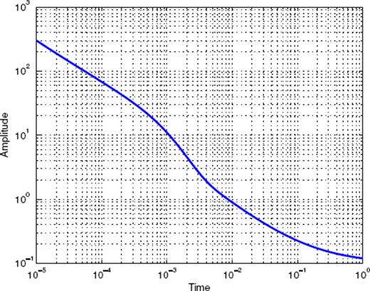
Let us first consider Fig. 1, which shows the binned stacked series obtained for main shock magnitudes in the interval [4;4.5]. The many data points represent the binned series for all values of the binning factor α. The aftershock decay rate does not appear to be a pure power law, and displays rather large fluctuations. A first scaling regime seems to hold from 10⁻⁵ to 4 × 10⁻⁴ yr, followed by a second scaling regime up to 5 × 10⁻³ yr, then a third scaling regime which progressively fades into the background rate. Note the similarity of this time-series with the synthetic one shown in Fig. A7 in the Appendix, which is the sum of three different contributions (a gamma law, a power law, and a constant background term). Fig. 2 shows the Scaling Function Analysis coefficient (SFAC) of the corresponding set of aftershocks. The two solid lines correspond, respectively (from top to bottom) to n_B = 0 and 3.

Figure 1.

Binned stacked time-series of sequences triggered by main events with magnitudes M within the interval [4;4.5] in the SCEC catalogue, including the Brawley zone. This plot shows all binned series corresponding to all the 20 binning factors from α = 1.1 to 3.

Open in new tabDownload slide

Figure A7.

Time-series defined as the sum of a Gamma function, an Omori law and a constant background term.

Open in new tabDownload slide

Figure 2.

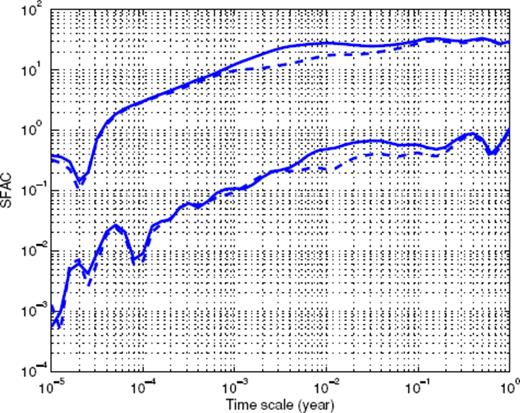
Scaling function analysis coefficient (SFAC) of the time-series shown in Fig. 1. The two top curves correspond to n_B = 0, the bottom curves to n_B = 3. The solid curves refer to the data sets which include events in the Brawley zone. The dashed curves correspond to the data sets excluding those events.

Open in new tabDownload slide

The first important observation is that the shape of the SFAC as a function of scale is independent of n_B. This means that the term B(t) in (16) is certainly quite close to a constant. Secondly, we clearly observe that a first power-law scaling regime holds for timescales within [5 × 10⁻⁵; 5 × 10⁻³] (for n_B = 0 and similarly with the same exponent for n_B = 3). The exponent being ≃ 0.6, this suggests a p-value equal to p = 0.4. Each curve then goes through a maximum, followed by a decay, and then increases again. This behaviour is strikingly similar to the one shown in Fig. A8 in the Appendix. This suggests that the time-series shown in Fig. 2 may be a mixture of several different contributions, such as gamma and power laws. This simple example shows that the SFA provides a clear evidence of a mixture of aftershock sequences with different nature within the same stacked series-a fact that has never been considered in previous studies of the same or of other catalogues.

Figure A8.

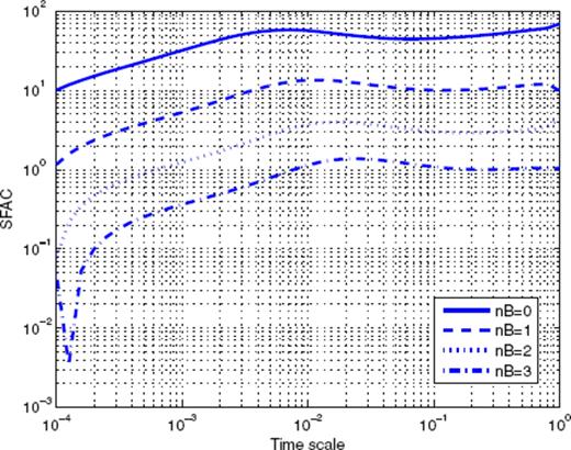
Scaling function analysis of the time-series shown in Fig. A7. Each curve corresponds to a given value of n_B used to build the corresponding MSF.

Open in new tabDownload slide

We thus tried to identify in the SCEC catalogue those events that may be responsible for the non-Omori behaviour revealed by the SFA. After many trials, we were able to locate a very small spatial domain in which many short-lived sequences occur. This zone is located within [−115.6°; −115.45°] in longitude and [32.8°;33.1°] in latitude. It is located in the Imperial Valley area, and extends northwest from the Imperial fault to the San Andreas fault. It corresponds to the Brawley seismic zone, and its seismicity is known to be dominated by short-lived earthquake swarms (Habermann & Wyss 1984). In the remaining of the SCEC catalogue analysis, we decided to exclude any sequence triggered by a shock in this small zone. The impact of excluding the Brawley area is illustrated in Fig. 2 with the two dashed lines, which can be compared with the two continuous lines (which correspond to the full catalogue). Excluding the Brawley area significantly changes the scaling properties, and one can now measure an exponent p = 0.80 for timescales larger than 10⁻³ yr.

4.1.3 Results on the cleaned SCEC catalogue using the binned stacked series

Following our identification of the anomalous Brawley zone, we removed all events in the aftershock catalogue associated with this zone, and launched again our analysis of the binned stacked sequences using our three independent methods of analysis.

Fig. 3 shows the binned stacked series for the SCEC catalogue. Each series corresponds to a given magnitude range. For each magnitude range, for the sake of clarity, we chose to plot only one binned time-series, corresponding to a given α-value. The α-value we choose is the one for which the obtained p-value is the closest to the average p-value over all α values for that magnitude range. The solid lines show the fits of the corresponding series with formula (15). For each magnitude range, the average p-values and their standard deviations are given in Table 1. Fig. 4 shows the corresponding dependence p(M) of the p-value as a function of the magnitude of the main shocks. The dependence p(M) is well fitted by the linear law p(M) = 0.11M+ 0.38. This relationship is very close to the dependence p(M) = 0.10M+ 0.37, reported by Ouillon & Sornette (2005). Despite the differences in the catalogues and in the general methodology, we conclude that the results are very stable and confirm a significant dependence of the exponent of the Omori law as a function of the magnitude of the main shock.

Table 1.

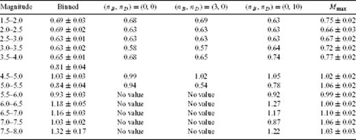
p-values for the SCEC catalogue obtained from fitting binned stacked sequences with formula (15) (second column), with the SFA (third to fifth columns) and with monitoring M_max (last column). (n_B, n_D) correspond to the parameters used to define the mother scaling function (see the Appendix for definitions). p(M) values in the second, fifth and last columns are plotted in Fig. 4.

Open in new tabDownload slide

Figure 4.

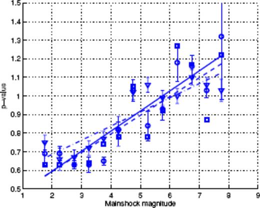
p(M) values obtained for the SCEC catalogue with fits of binned time-series (squares-second column of Table 1), Scaling Function Analysis (circles-fifth column of Table 1) and monitoring of M_max (triangles-last column of Table 1). Continuous, dashed and dot-dashed lines stand for their respective linear fits.

Open in new tabDownload slide

The events within the SCEC catalogue we used are located within [−121.877°; −114.005°] in longitude and [31.3283°;38.4967°] in latitude. Recently, Helmstetter et al. (2007) showed that the completeness magnitude in Southern California displayed spatial variations, especially near the boundaries of that area where larger magnitude detection thresholds are observed. We thus performed a second binned time-series analysis, taking account only of events occurring within [−120;−116] in longitude and [34;38] in latitude. The results we obtained provide a relationship p(M) = 0.11M+ 0.31, which is in good agreement with the one we obtained using the whole catalogue. The other methods of analysis were thus applied to the previous, larger catalogue too.

4.1.4 Results obtained with the SFA method

The SFAC as a function of scale are displayed in Figs 5–7. In each of these figures, we analyse the stacked aftershock time-series for main shocks in a small magnitude interval, and vary the two parameters n_B (which controls the ability of the SFA to filter non-Omori dependence) and n_D (which controls the weight put to early times in the stacked aftershock sequence, the larger n_D is, the weaker is the influence of the early times in the analysis). The parameter n_D is defined in the Appendix as the maximum order of the derivatives of the ‘mother scaling function’Ψ of the SFA method which vanish at t = 0. Typically, we consider the following values: n_B = 0 and 3 and n_D = 0 and 10. In the set of Figs 5–7, the upper solid curve corresponds to n_B = 0 and n_D = 0, the dashed curve corresponds to n_B = 3 and n_D = 0, while the lower solid curve corresponds to n_B = 0 and n_D = 10. One can check that the value of n_B has very little influence on the shape of the curves, suggesting that the contribution of the background rate is practically constant with time. This in turn validates our aftershock selection procedure, as it shows that aftershock sequences are at most very weakly contaminated by sequences triggered by previous events. The straight dashed lines show the power-law fit of the SFAC as a function of timescale. In some cases, different scaling regimes hold over different scale intervals, so that more than one fit is proposed for the same time-series (see for instance, Figs 5e and 6a). Note that the fitting interval has a lower bound at small scales due to the roll-off effect observed in the time domain. At large timescales, several features of the time-series define the upper boundary of the fitting interval. The first feature is of course the finite size of the time-series, as discussed in the Appendix. The other property is related to the occurrence of large secondary aftershock sequences that appear as localized bursts in the time-series and distort it. For example, consider the time-series corresponding to the main shock magnitude range [1.5;2] in Fig. 3, for which one can observe the occurrence of a burst at a time of about 6 × 10⁻² yr. This corresponds to a break in the power-law scaling of the SFAC at timescales of about 10⁻¹ yr. We thus only retained the p-values measured using timescales before such bursts occur. As the magnitude of the main shocks increases, the roll-off at small timescales extends to larger and larger timescales, so that the measure of p proves impossible when n_D = 0. This is the reason why we consider the p-value measured with n_D = 10 and n_B = 0 as more reliable, especially for the large main shock magnitudes.

Figure 5.

SFA method applied to the SCEC catalogue: main shock magnitudes vary within [1.5;2] (plot a) up to [4;4.5] (plot f). In each plot, the upper solid curve corresponds to n_B = 0 and n_D = 0, the dashed curve corresponds to n_B = 3 and n_D = 0, while the lower solid curve corresponds to n_B = 0 and n_D = 10. Occurrences of large bursts in the time-series sometimes interrupt the power-law scaling (see plots a, b and e).

Open in new tabDownload slide

Figure 6.

SFA method applied to the SCEC catalogue: main shock magnitudes vary within [4.5;5] (plot a) up to [7;7.5] (plot f). In each plot, the upper solid curve corresponds to n_B = 0 and n_D = 0, the dashed curve corresponds to n_B = 3 and n_D = 0, while the lower solid curve corresponds to n_B = 0 and n_D = 10. The roll-off of aftershock time-series at small timescales breaks scaling down and imposes to choose n_D = 10.

Open in new tabDownload slide

Figure 7.

Same as Fig. 6 for M within [7.5;8].

Open in new tabDownload slide

The estimation of reliable error bars with the SFA method is not as obvious as for the other methods, as different (n_B, n_D) couples describe different scaling functions, that is, different methods to estimate p. For example, the binned stacks method previously defined indeed belongs to the general family of SFA methods. In that case, the mother scaling function is a simple square function, so that it doesn't filter out any background term. Using different values of the binning factor α changes the scale of analysis, but not the basic properties of the analysed time-series. In the SFA method that we defined in Section 3.3, changing n_B and n_D filter out some different parts of the signal itself before we unearth its scaling properties through a linear fit in log-log scales. Each mother scaling function Ψ thus defines a unique tool in itself. Table 1 gives an idea of the variation of p obtained with different scaling functions (hence different methods). Note that they agree very well with those obtained with the direct binning and fitting approach.

Fig. 4 shows the p-values obtained with n_B = 0 and n_D = 10 as a function of M. We plot those results without error bars (for reasons given above). A linear fit gives p(M) = 0.10M+ 0.40, in excellent agreement with the results obtained using the direct fit to the binned stacked series.

4.1.5 Results obtained with the maximum magnitudes method

We now present the results obtained with the analysis using maximum magnitudes in logarithmic binned time-intervals. As this method focuses only on extreme events, the corresponding plots of the maximum magnitude as a function of time elapsed since the main shock display larger fluctuations than the ones given by the two other methods. Fig. 8 shows such plots for main shock magnitudes within [2;2.5] (square symbols) and within [7;7.5] (circles) for a common ratio α = 1.7 used to bin the time intervals. For the largest magnitude range, a clear decrease of the maximum magnitude with time is observed, with a slope of about −0.05. Assuming that b = 1, this yields p = 1.05. Note that the scaling law extends down to a very small time slightly less than 2 min, whereas the binned time-series analysis used previously allowed to observe power-law scaling only down to about 1 month. For the smallest magnitude range, we can observe that M_max increases with time, with a slope of about 0.41. It follows that p = 1 − 0.41 = 0.59, and the scaling range extends down to a time of about 0.3 s. We also see that there are two very clear outliers at magnitudes M_max larger than 7. They can thus be very easily discarded when performing the fit to find p. Indeed, for main shock magnitudes lower than 3, we fitted the corresponding data up to a time t = 10⁻³ yr to remove the possible influence of the constant background. The results obtained using 20 different values of α for all magnitude ranges are gathered in Table 1. Note that they compare very well with those obtained with the two other methods. They are plotted with error bars in Fig. 4. A linear fit gives p = 0.08M+ 0.53, in good agreement with previous results on the same catalogue. Discarding the smallest and the largest magnitude ranges gives an even better agreement with p = 0.10M+ 0.44. The significance of the largest magnitude range will be discussed later in this paper.

Figure 8.

Time evolution of extreme aftershock magnitudes following main shocks with magnitudes within [2;2.5] (squares) and within [7;7.5] (circles).

Open in new tabDownload slide

4.2 JMA catalogue

The JMA catalogue used here extends over a period from 1923 May to 2001 January inclusive. We restricted our analysis to the zone (+130°E to +145°E in longitude and 30°N to 45°N in latitude), so that its northern and eastern boundaries fit with those of the catalogue, while the southern and eastern boundaries fit with the geographic extension of the main Japanese islands. This choice selects the earthquakes with the best spatial location accuracy, close to the inland stations of the seismic network. In our analysis, the main shocks are taken from this zone and in the upper 70 km, while we take into account their aftershocks which occur outside and at all depths.

Our detailed analysis of the aftershock time-series at spatial scales down to 20 km reveals a couple of zones where large as well as small main events are not followed by the standard Omori power-law relaxation of seismicity. The results concerning these zones will be presented elsewhere. Here, we simply removed the corresponding events from the analysis. The geographical boundaries of these two anomalous zones are [130.25° E; 130.375° E]×[32.625° N; 32.75° N] for the first zone, and [138.75° E; 139.5° E]×[33° N; 35° N] for the second one (the so-called Izu islands area). This last zone is well known to be the locus of earthquakes swarms (see for example Toda et al. 2002), which may explain the observed anomalous aftershock relaxation. We have been conservative in the definition of this zone along the latitude dimension so as to avoid possible contamination in the data analysis which would undermine the needed precise quantification of the p-values.

The completeness of the JMA catalogue is not constant in time, as the quality of the seismic network increased more recently. We computed the distribution of event sizes year by year, and used in a standard way (Kagan 2003) the range over which the Gutenberg-Richter law is reasonably well obeyed to infer the lower magnitude of completeness. For our analysis, we smooth out the time dependence of the magnitude threshold M_c above which the JMA catalogue can be considered complete from roughly M_c(1923 − 1927) = 6, to M_c(1927 − 1930) = 5.5, M_c(1930 − 1962) = 5, M_c(1962 − 1993) = 4.5, M_c(1993 − 1995) = 3.5 and M_c(1995 − 2001) = 2.5. This time-dependence of the threshold M_c(t) will be used for the selection of main shocks and aftershocks. The assumed value of events location uncertainty Δ has been set to 10 km.

4.2.1 Binned stacked times series

For the JMA catalogue, 12 magnitude intervals were used (from [2.5;3] to [8;8.5]). Fig. 9 shows the 12 individual stacked aftershocks time-series and their fits (using a value for the binning factor α determined as described above for the SCEC catalogue). Fig. 10 plots the exponent p averaged over the 20 values of α as a function of the middle value of the corresponding magnitude interval. These values are also given in Table 2. A linear fit gives p = 0.06M+ 0.58 (shown by the solid straight line in Fig. 10). The p-value thus seems less dependent on the main shock magnitude M than for the SCEC catalogue.

Figure 9.

Binned stacked series of aftershock sequences in the JMA catalogue for various magnitude ranges (from [2.5;3] at the bottom to [8;8.5] at the top by steps of 0.5). The solid lines show the fits of formula (eq. 15) to the individual time-series. All curves have been shifted along the vertical axis for the sake of clarity.

Open in new tabDownload slide

Figure 10.

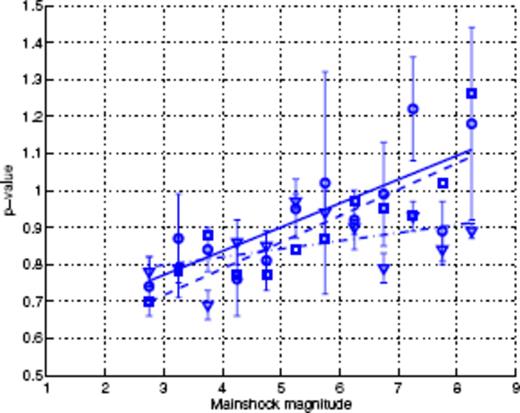
Exponents p(M) of the Omori law obtained for the JMA catalogue with different methods (stacked binned method and SFA), with the corresponding fits: binned time-series (squares-second column of Table 2), Scaling Function Analysis (circles-fifth column of Table 2) and monitoring of M_max (triangles-last column of Table 2). Continuous, dashed and dot-dashed lines stand for their respective linear fits.

Open in new tabDownload slide

Table 2.

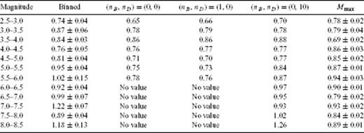
p-values for the JMA catalogue obtained by fitting binned stacked sequences (second column), with the SFA (third to fifth columns) and with monitoring M_max (last column). (n_B, n_D) correspond to the parameters used to define the mother scaling function. p(M) values in the second, fifth and last columns are plotted in Fig. 10.

Open in new tabDownload slide

4.2.2 SFA method

We also applied the SFA method to the same data set. We checked that the resulting curves were not dependent on the value of n_B, suggesting that the background term is constant. Figs 11 and 12 show the SFAC as a function of scale for different values of (n_B, n_D): (0, 0) (upper solid curve), (3, 0) (dashed curve), and (0, 10) (lower solid curve). One can observe that some of them exhibit a more complex scaling behaviour than found for the SCEC catalogue. This may reveal a complex mixture of sequences with different properties (see for example, Figs 11e and 12a which exhibit two characteristic timescales of about 10⁻³ and 10⁻¹ yr), despite our efforts to exclude zones that have a large number of swarms. The characteristic scales disappear with n_D = 10, but this may just be due to the strongly oscillating character of the filter and therefore of the SFAC which may mask its local maxima. Table 2 and Fig. 10 report the corresponding measured exponents. There is a general agreement between the p-values measured using different sets of parameters. Using the set of p-values corresponding to n_B = 0 and n_D = 10, we obtain the following dependence of the p-value as a function of the magnitude M of the main shocks: p = 0.07M+ 0.50. Excluding the largest magnitude range leads to a weaker dependence: p = 0.05M+ 0.58. Note that the dispersion of data points around the best-fitting line is much smaller for the p-values obtained by the SFA method. This thus confirms the weaker dependence of p as a function of M for the JMA catalogue. Our SFA suggests that this weaker dependence may have to do with the presence of many swarms in the Japanese catalogues, as our methodology has allowed us to diagnose the existence of mixtures of aftershock relaxation regimes, probably swarms and standard Omori standard sequences.

Figure 11.

SFA method applied to the JMA catalogue for main shock magnitudes M within [2.5;3] (plot a) up to [5;5.5] (plot f). The upper solid curve corresponds to n_B = 0 and n_D = 0, the dashed curve corresponds to n_B = 3 and n_D = 0, while the lower solid curve corresponds to n_B = 0 and n_D = 10. Note the existence of characteristic scales (as in plot e).

Open in new tabDownload slide

Figure 12.

Same as Fig. 11 for M within [5.5;6] up to [8;8.5].

Open in new tabDownload slide

4.2.3 M_maxmethod

The results of the fits are gathered in Table 2 and plotted in Fig. 10 with error bars. It is worth noticing that the magnitude dependence of p is observed to be much weaker than with other methods, as we now get p = 0.02M+ 0.72. The scale invariance properties of this catalogue thus suggest an almost monofractal scaling (as p is constant with M). Further work is needed to understand the role of swarms in those scaling properties.

4.3 The Harvard CMT catalogue

The worldwide CMT Harvard catalogue used here goes from 1976 January to 2006 August inclusive. This catalogue is considered to be complete for events of magnitude 5.5 or larger. We thus removed events below this threshold before searching for the aftershocks. Due to the rather small number of events in this catalogue, we did not impose any limit on the depth of events. The assumed value of location uncertainties has been set to Δ = 10 km. Note that instead of using the hypocentre location as we did for the two other catalogues, we considered the location of the centroid, which is certainly closer to the centre of the aftershock zone.

4.3.1 Binned stacks

For the Harvard catalogue, seven magnitude intervals were used from [5.5;6] to [9;9.5] (the [8.5;9] interval being empty). The binned stacked times series for the [5.5;6] magnitude range are shown in Fig. 13, using all values of the binning factor α. The underlying decay law is obviously not of Omori-type, which suggests that it is the result from the superposition of different distributions. We attribute the different behaviour of the [5.5;6] magnitude range to the fact that the corresponding times series contain many events occurring at mid-oceanic ridges, where many swarms are known to occur. As very few events of magnitude >6 occur in this peculiar tectonic settings, swarms (from the mid-ocean ridges) do not contaminate too much the time-series associated with larger magnitude main shocks. We will see below that the SFA confirms this intuition, and doesn't provide any evidence of a power-law scaling for the [5.5;6] magnitude range while the other magnitude ranges (except the largest) give reliable estimates for the Omori exponent p.

Figure 13.

Binned stacked time-series of sequences triggered by main events in the Harvard CMT catalogue with M within [5.5;6]. This plot features binned series corresponding to all α values.

Open in new tabDownload slide

Fig. 14 shows the six remaining stacked aftershocks time-series and their fits (constructed as in Figs 3 and 9). One can clearly observe Omori-like behaviours. The corresponding p-values are reported in Table 3 and in Fig. 15 as a function of the main shock magnitudes M. The linear fit of the dependence of p as a function of M gives p(M) = 0.16M− 0.09. The magnitude dependence of M is thus much larger than found in Southern California but we have to consider that the magnitude range over which the fit is performed is much more restricted than that for the SCEC catalogue, leading to larger uncertainty. Note that the [9;9.5] magnitude range displays an unusual small p-value of 0.69. This may be due to the fact that we are still in the roll-off time range, or to the very limited amount of data as only one main shock occurred in that magnitude range. For this reason, we excluded it in the estimation of the p(M) relationship. See the last section of this paper for a discussion about large magnitude events and the significance of the p-value of time-series triggered by such events.

Figure 14.

Binned stacked series of aftershock sequences in the Harvard catalogue for various magnitude ranges. Magnitude ranges are, from bottom to top: [6;6.5], [6.5;7], [7;7.5], [7.5;8], [8;8.5] and [9;9.5]. The solid lines show the fits to the individual time-series. The [9;9.5] magnitude range displays an unusual small p-value of 0.69 (see text for further discussion of this anomaly in comparison with the other magnitude ranges). All curves have been shifted along the vertical axis for the seek of clarity.

Open in new tabDownload slide

Table 3.

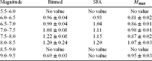
p-values for the HARVARD catalogue obtained by fitting the binned stacked sequences (second column), with the SFA (third column) and with monitoring M_max (last column). p(M) values are plotted in Fig. 15.

Open in new tabDownload slide

Figure 15.

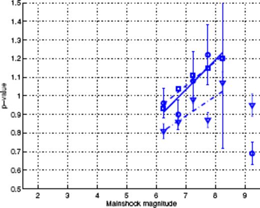
Dependence of the Omori exponent p as a function of the main shock magnitude M obtained for the Harvard CMT catalogue with fits of the binned time-series (squares-second column of Table 3), Scaling Function Analysis (circles-fifth column of Table 3) and monitoring of M_max (triangles-last column of Table 3). Continuous, dashed and dot-dashed lines stand for their respective linear fits.

Open in new tabDownload slide

4.3.2 SFA method

Figs 16 and 17 present the dependence of the SFAC as a function of scale for the different main shock magnitude ranges. Due to the incompleteness (roll off) effect and to the rather large value of magnitude M_c = 5.5 of completeness, one can observe in Fig. 14 that the power-law scaling do not hold at scales smaller than about 10⁻³ yr. This thus prevents us from using the SFA method with n_D = 0 to measure an accurate value of the Omori exponent p. We thus first checked that, using n_D = 0, the shape of the SFAC curves is independent of n_B. We then set n_B = 0 and considered different values of n_D = 0, 2, 4 and 8. Larger values of n_D lead to strongly oscillating SFAC as a function of scale, which are difficult to interpret. Only one fit (straight dashed line) is shown in each figure, and the corresponding p-values are gathered in Table 3 and plotted in Fig. 15. We chose the fits with a non-zero n_D value such that the SFAC curve does not oscillate too much. We can visually check that the chosen fit is compatible with other non-zero values of n_D, as well as with the extrapolation to scales where the SFAC is oscillating. Due the small amount of data, no p-value could be determined for the [9;9.5] range, as the SFAC is strongly oscillating for any value of n_D (see Fig. 17). Concerning the smallest magnitude range ([5.5;6]), one can note the existence of two characteristic scales so that no power-law scaling holds. Those scales are of the order 10⁻² and 10⁻¹ yr. Fig. 16(a) should be compared with Figs 11(e) and 12(a) for similar behaviours of the SFAC observed in the JMA catalogue. This strengthens our conjecture that the JMA catalogue we used still contains numerous swarms that may alter the quality of our results.

Figure 16.

SFA method applied to the Harvard CMT catalogue for main shock magnitudes M within [5.5;6] (plot a) up to [8;8.5] (plot f). Note the existence of two characteristic scales in plot (a). The parameter n_B is set to zero and in each plot the four curves correspond to different values of n_D as indicated in the insert panel of plot (a).

Open in new tabDownload slide

Figure 17.

Same as Fig. 16 for M within [9;9.5]. As the dependences of the SFAC as a function of scale are too strongly oscillating, we do not provide any fit.

Open in new tabDownload slide

Excluding the largest magnitude range, a linear fit of the dependence of the Omori exponent p as a function of the main shock magnitude M gives p(M) = 0.13M+ 0.14. This fit is different from that obtained with the binned stacking method, probably due to the limited magnitude range available for the Harvard catalogue. In any case, both methods confirm a strong magnitude dependence of the Omori exponent p.

4.3.3 M_maxmethod

The results are also given in Table 3 and in Fig. 15. The p-values we obtain with this method are slightly smaller than those obtained with the two other methods. If we take account of all data, we get p = 0.05M+ 0.51, that is, a much weaker dependence than previously found. If we exclude the largest magnitude datapoint, we now obtain p = 0.11M+ 0.15. The discrepancy between all three method could be due to the more limited magnitude range available for the linear fit. It is important to note that the p-value for the largest magnitude range is now p = 0.95 whereas the binned stacks method provided p = 0.69. This proves the necessity to use a method to shortcut the problem of missing events. Fig. 14 suggests that the background term is significant for all magnitude ranges. This could explain why the p-values tend to be lower than those obtained with other methods. We thus monitored the time evolution of extreme magnitudes, neglecting times larger than 0.1 yr, except for the largest magnitude range. We then observed p = 0.05M+ 0.58 when including the largest magnitude range and p = 0.11M+ 0.17 when removing the largest magnitude range. The influence of the background term is thus quite weak.

5 Concluding Remarks

We have introduced three methods to analyse the time-relaxation of aftershock sequences. One is based on standard binning methods, the second one is inspired by the wavelet transform adapted to the present problem leading to the SFA method, and the third one uses the monitoring of the occurrence times of large magnitude events. We analysed three different catalogues using a very simple declustering technique based on the definition of a magnitude-dependent space-time window for each event. The SFA method showed that this declustering method is sufficient, as aftershock sequences of small events are not contaminated by aftershock sequences triggered by previous larger events. All methods yield very similar results for each of the three catalogues, suggesting that our results are reliable. They confirm the results of the binning method already presented by Ouillon & Sornette (2005), showing that the p-value of the Omori law increases linearly as a function of the magnitude of the main shock for the SCEC catalogue. Those results are also in good agreement with the p(M) dependence measured for the Harvard CMT catalogue. The magnitude dependence of p is much less obvious for the Japanese JMA catalogue, but the SFA method clearly diagnosed that a rather significant number of swarm sequences are still mixed with more standard Omori-like sequences, so that the obtained results should not be considered as representative of the latter. Overall, the extensive analysis presented here strengthens the validity of the major prediction of the MSA model, namely that the relaxation rate of aftershock sequences is an Omori power law with an exponent p increasing significantly with the main shock magnitude.

We now discuss a few relevant recent results obtained by other groups in the light suggested by our present analysis and the MSA model.

Ziv & Rubin (2003) study the decay rate of earthquake activity on a fault subjected to a positive stress step. In their numerical model, they consider a 2-D planar fault divided in small patches able to fail according to the rate-and-state friction law. The failure of a patch redistributes stress on the whole fault according to linear elasticity laws, so that the stress interaction is always positive: the stress decreases at the location of the ruptured patch, but increases everywhere else on the fault. This is thus different from our theoretical model where both positive and negative stress increments are possible (as is the case in multiple, non-coplanar fault networks). Ziv & Rubin (2003) then simulate an earthquake catalogue on such a fault subjected to a far-field loading until the system reaches a steady-state. The fault is then subjected to a positive stress step, which effect is to increase the seismicity rate before it decays with time to a background rate. Ziv & Rubin (2003) then show that the shape of the temporal decay law doesn't depend on the introduction or the suppression of elastic interactions between fault patches. This apparently questions our findings that the introduction of multiple interactions coupled with the non-linearity of the earthquake nucleation process leads to a change of the shape of the aftershock decay law (as the p-value should either increase or decrease when one switches on elastic interactions). But one must realize that both problems are of fundamentally different natures. In the case of Ziv and Rubin, the system first reaches a self-organized steady-state, and is then subjected to an exogenous stress step fluctuation. It is exogenous in the sense that it is not the consequence of the building of interactions and correlations of the stress field on the fault due to previous seismic activity. In our model, we look at the decay of seismic activity after events that all result from the interactions between all previous events. In that sense, we are looking at seismicity decay rates that follow endogenous fluctuations. In a recent paper, Sornette & Helmstetter (2003) showed theoretically that in the case of the linear ETAS model, endogenous and exogenous fluctuations should be followed by different decay rates of activity. In addition, in the presence of a multfractal p(M) dependence for endogenous shocks, it has been shown that the response to an exogenous shock should be reveal a single power law decay associated with the time-memory kernel of the non-linear process (Sornette et al. 2003). The difference between the results of Ziv & Rubin (2003) and ours is thus no surprise at all.

This reflection on endogenous and exogenous types of fluctuations may also shape the interpretation of the p-values of aftershock series triggered by very large events. For example, the Sumatra earthquake certainly constitutes a very singular event that should be considered with a lot of caution before drawing reliable conclusions. This event propagated over a length of about 1200 km, which is thus 14 times the size of the largest event in the SCEC catalogue (the M = 7.5 Kern County event), and 1.5 times the linear size of the whole Southern California catalogue. The Sumatra event thus certainly ruptured across many different tectonic domains or subdomains, which experienced different, possibly uncorrelated, stress trajectories. This phenomenology is difficult to handle in a theoretical model, as it means that this event certainly nucleated in a given domain due to the influence of previous earthquake activity (and thus endogenous stress fluctuations), but propagating on such a long distance across possibly uncorrelated domains also means that this event in turn constituted an exogenous stress fluctuation in those other domains. The resulting catalogue of aftershocks may thus be a mixture of events triggered by an endogenous process and of events triggered by an exogenous process. Note that this event is so large that the triggered sequence might be dominated by the last type of events, hence explaining a low p-value compared to our p(M) prediction. Anyway, this simple argument shows that the scaling of aftershock sequences triggered by very large events may strongly depart from the model we propose. If this view is correct, we still have to define the upper spatial size of events below which all events can be considered as endogenous stress fluctuations. For instance, the Sumatra earthquake belongs to the part of the distribution of magnitudes which departs significantly from the pure Gutenberg-Richter law. This reveals that finite-size effects and other possible mechanisms are kicking in to modify the physics for such large magnitude events.

In a recent paper, Peng et al. (2007) proposed a new methodology to identify aftershocks occurring in the first 900 s after a main event in order to get a better estimation of the decay rate of aftershock activity at very short timescales, generally badly sampled in standard catalogues. They thus selected a set of 82 main events located in Japan, with magnitudes in the range [3;5]. Stacking all sequences, they then showed that the p-value for early aftershocks is lower (p = 0.58) than for late aftershocks (p = 0.92). It is important to note that the time boundary between these two regimes is exactly 900 s, that is, the value separating the time intervals in which the two methods for selecting the aftershocks are applied. Rather than reflecting a genuine cross-over in the dynamics of aftershock generation, the observed change of the p-value might therefore reflect the existence of the two different sampling techniques. The results obtained by Peng et al. (2007) can be compared to ours only for the late aftershocks that occurred more than 900s after the main events. In fig. 11 of Peng et al. (2007), the p-values are reported for the different groups of late aftershocks (plotted using black triangles). This figure can be compared to ours by noticing that groups 4–7 of Peng et al. (2007) correspond to stacked sequences originating from main shocks with different magnitude ranges (respectively [3;3.5], [3.5;4], [4;4.5] and [4.5;5]). One clearly sees in fig. 11 of Peng et al. (2007) that p increases linearly with M, with p≃ 0.13M+ 0.37. This linear fit predicts p-values larger than those we obtained for the JMA catalogue, but we should stress that the initial data sets are quite different: the number of sequences is much larger in our case and they cover a much larger area than in the aftershock sequences used by Peng et al. (2007). Another difference is that Peng et al. (2007) discarded events shallower than a 2 km depth, in order to remove events of volcanic origin (swarms). Anyway, we find it encouraging that an independent work performed on a different data set with a very different approach seems to converge to a result similar to our's.

Recently, Helmstetter & Shaw (2006) and Marsan (2006) showed that Dieterich's model could predict p-values less than 1, when accounting for a heterogeneous stress distribution. The relevance of this a priori very interesting prediction must be tempered by the fact that those papers focus only on spatial areas that are predicted to be unloaded by usual smooth dislocation or crack models of the main shock, as the authors wish to explain how a static stress triggering model can both predict the absence of stress shadows at short timescales and their emergence much later in time. Their basic ingredient is that the rupture plane undergoes an average stress drop, but as the spatial structure slip pattern is self-similar, it can also display very large fluctuations of the stress field (which is the derivative of the displacement field). Coupling the variance of the stress field with the rate-and-state friction law allows them to show that if the variance is large enough, then some patches are able to nucleate aftershocks that obey the Omori-Utsu law. The larger the variance, the closer to 1 is p. If the slip pattern is smooth, then the fault plane displays immediate quiescence. If not, the quiescence is delayed to times following the aftershocks sequence. This mechanism seems to be robust with respect to the inclusion of interactions between events. An anonymous reviewer of this paper suggested that this mechanism could offer an alternative explanation for the variation of p with the main shock rupture length: the larger the main shock, the rougher the stress field at the nucleation scale, the closer to 1 is the p-value. Indeed, this idea stems from the conclusion of Lapusta & Rice (2003) according to which the nucleation length of any earthquake is the same whatever the size of the event. While quite seducing at first sight, it is certainly too early to claim that stress heterogeneity is the source of the magnitude-dependence of the p-value. Indeed, Helmstetter & Shaw (2006) and Marsan (2006) both focus on areas where an average stress decrease is predicted, but do not take account of areas where stress is predicted to increase. They thus certainly neglect most of the aftershocks that occur in a sequence (whereas they dominate the scaling of our time-series). Moreover, their respective models are unable to explain p-values larger than 1. Helmstetter & Shaw (2006) consider an exponential distribution of stress values, and derive a theoretical expression linking p to the standard deviation of the stress field. They indeed predict that the p-value should be infinitely negative if the standard deviation tends to zero. Marsan (2006)'s framework predicts that p should decrease very strongly and become negative when approaching M₀, the main shock magnitude corresponding to the nucleation length. Moreover, both papers assume that most of the aftershocks occur on the fault plane itself, where an average stress drop is observed. It is however still unclear if most of the aftershocks really occur on the ruptured plane itself, where the stress decreases on average, or on its perimeter, where elastostatics predicts a large average stress increase. If the latter holds, the model of Helmstetter & Shaw (2006) and Marsan (2006) would only concern a minority of events. Finally, we would like to point out that those models do not specifically predict any linear p(M) relationship, nor do they take account of events that occurred before the main shock.

We would like to conclude by confirming the importance of taking into account stress heterogeneity, as it is indeed included in the MSA model. One of the key ingredients of the MSA model is that each main shock of magnitude M generates an immediate burst of activity of the order of 10^qM events (with q > 0), so that right after that main shock, the stress field at any spatial location is the sum of approximately 10^qM random stress fluctuations occurring within a very short time interval. An alternative approach is to consider the main shock alone as the only source of such random stress fluctuations. If we consider that the slip pattern over the rupture plane is self-similar, the fault plane after the main rupture consists of a set of random slip fluctuations. The larger the rupture plane, the larger the number of such fluctuations. Those slip fluctuations are mediated as stress to the surrounding medium via an elasto-viscoplastic Green's function. In the simplest linear elastic case, the total stress variation due to the main shock at any location (i.e. on the rupture plane or outside of it) is thus the sum of all those random stress fluctuations created by the slip fluctuations, each fluctuation being either positive or negative. Assuming that the number of random slip fluctuations on a rupture plane scales with magnitude as 10^qM, we now have a clearer picture of the origin of this term. For example, if we assume that the total number of slip fluctuations on the fault plane is proportional to its area, we get q = 1. We thus see that the MSA model indeed includes the concept of stress heterogeneity on a fault plane (intimately linked to the rupture dynamics of single events) as well as the whole history of the stress field, which ultimately yields a linear dependence of the p-value as a function of M. To the best of our knowledge, the MSA model is the only framework which predicts this remarkable multifractal property.

Acknowledgments

We thank Massimo Cocco for his efficient mediation between us and the reviewers.

References

Appendix

Appendix: The Scaling Function Analysis

The SFA described in this Appendix develops a fitting procedure that removes the impact of non-Omori law terms in expression (17) as described by the polynomial expansion describing a tectonic background contribution and the impact of aftershock sequences of main events preceding the main shock under investigation.

A1 Construction of the mother scaling functions (MSF)

The first step in developing the SFA, which is inspired from the well-known wavelet transform, is to define a mother scaling function (hereafter MSF) that we shall name Ψ, and define the associated SFA coefficient C(s = 1) of the seismicity rate function N(t) by

(A1)

We then define a set of daughter scaling functions , where s is a timescale parameter chosen by the user (that should not be mistaken for the fluctuations of the stress described in the MSA model), and compute the associated SFA coefficients (hereafter SFAC)

(A2)

The parameter s allows to dilate or contract the MSF Ψ in the time domain, so that it focuses on the short or long timescales content of N(t) near the origin time t = 0. In the analogy with a wavelet transform, the SFAC is nothing but the wavelet coefficient measured at the time location t = 0 and timescale s. If we now assume that N(t) = A·t^−p+B(t), we have (using a simple change of variable):

(A3)

For a given stacked series, the first integral is independent of s, so that the variation of C(s) with s stems from two contributions: a power-law term with exponent 1 −p, plus a term depending on the shapes of B(t) and Ψ(t), and s. We shall now show how to choose function Ψ to allow an easy measurement of exponent p.

We choose the MSF so as to respect the following constraints. First of all, Ψ is designed to analyse the scaling properties of aftershock sequences, that is, of sequences that are triggered shortly after a main shock. It is thus rational to choose Ψ so that it is defined only for positive times, and that its modulus decays rather quickly with time (so that it focuses on short-term rather than long-term scales). This last ingredient is also necessary as the integrals in eq. (A3) run over an infinite interval whereas seismic catalogues are necessarily bounded and our aftershock time-series are selected with a duration T = 1 yr. A fast decay of the MSF thus ensures that those boundary effects will have very little influence on our computations on real data. Second, the power-law scaling behaviour of C(s) results from the theoretical singularity of N(t) at t = 0. In real catalogues, of course, the seismicity rate does not diverge at small times, and one rather observes a roll-off of N(t), mainly due to the incompleteness of the catalogue. The Omori law thus breaks down for too short times, so that the scaling analysis presented in eq. (A3) doesn't hold. In order to circumvent this effect, we impose that Ψ(t = 0) = 0, so that aftershocks occurring at short times will have a negligible weight in the computation of C(s), preserving the announced scaling properties of the SFAC. Third, in order to measure p more easily, we impose that Ψ should filter out polynomials, so that the second term in the right-hand side of eq. (A3) gives a vanishing contribution to C(s). These three conditions are fulfilled with the following construction of Ψ:

(A4)

where the coefficients a and a_i (with i = 0, …, n_P), are determined as follows. For all integer values j = 0, …, n_B (where n_B is the degree of polynom B(t)), we impose that the function Ψ obeys the conditions

(A5)

If we find the corresponding coefficients a_i's, then our goal of removing the influence of the non-stationary background and of previous main shocks will be fulfilled as the second integral in the right-hand side of eq. (A3) will be exactly zero. Expression (A5) leads to

(A6)

where

(A7)

As eq. (A6) must hold for all j values between 0 and n_B, and as we also impose Ψ(0) = 0, the set of conditions (A6) defines a linear system of n_B+ 2 equations which can be solved to obtain the n_P+ 1 unknowns a_i. In order to obtain a non-degenerate solution, we impose n_P = n_B+ 2 and arbitrarily fix . The sign of is then chosen so that the most extreme value of the MSF is positive. The MSF is then normalized so that its maximum value is 1. In order to fully define the MSF, we still have to specify the two parameters a and n_B. In the remaining of this paper, we shall fix a = 5 yr⁻² (which ensures a good temporal localization of Ψ). As for the parameter n_B, it requires a specific discussion for each of the studied catalogues, as we don't know a priori what is the shape of the background term B(t). We will thus have to assume different values of n_B, define as many corresponding MSFs, and check if the SFAC function C(s) depends on n_B or not.

Fig. A1 shows the shape of the function Ψ for

Figure A1.

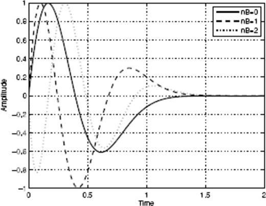
Plot of three different MSFs corresponding to different values of n_B.

Open in new tabDownload slide

• (i)

  n_B = 0 (n_P = 2) (which filters out only constant background terms B(t) = b₀).

• (ii)

  n_B = 1 (n_P = 3) (which filters out linear trends like B(t) = b₀+b₁t).

• (iii)

  n_B = 2 (n_P = 4) (which filters out quadratic trends like B(t) = b₀+b₁t+b₂t²).

The higher the order of the polynomial that needs to be filtered out, the more oscillating is the MSF. It is noteworthy that the shape of the MSF is independent of the precise shape of the function B(t) (and of its coefficients b_i). Only the degree n_B of the polynomial is needed to determine the corresponding MSF.

Imposing Ψ(0) = 0 decreases the influence of the incompleteness of real catalogues at short times after main shocks. However, for large main shocks, the corresponding roll-off in the Omori law can extend over days or weeks after the main shock, depending on the quality of the seismograph network at the time of occurrence of the main event and on the magnitude threshold for aftershocks selection in the catalogue. The MSF we just introduced may then prove unable to provide anything but spurious SFAC scaling estimations. We thus introduce additional constraints to build a suitable MSF with less sensitivity to the early times. Specifically, we impose in addition that all derivatives of Ψ up to order n_D vanish at t = 0. To obtain a non-degenerate system of equations determining the coefficients of the expansion Ψ, we have n_P = n_B+ 2 +n_D, and impose a_i = 0 for i = 0, …, n_D. Fig. A2 shows the MSFs for n_B = 0 and n_D = 0, 5, 10. At short times, Ψ takes negligible values over a time interval whose width increases with n_D. Aftershocks occurring within this interval will thus have a negligible contribution to the computation of the SFAC. We shall see in our analysis of real and synthetic catalogues that this set of MSF will provide much better estimates of p in a few peculiar situations.

Figure A2.

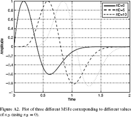
Plot of three different MSFs corresponding to different values of n_D (using n_B = 0).

Open in new tabDownload slide

Another advantage of using the SFA is that we do not need to bin the time-series of aftershock rates. Indeed, consider a given sequence of N_aft aftershocks occurring at successive times after their triggering main shock. By definition, the aftershock rate is a sum of Dirac functions

(A8)

which yields the SFAC

(A9)

according to the definition (A2). The estimation of C(s) is a simple discrete sum without any need for some intermediate manipulation of the data. The p-value is then retrieved with a simple linear fit of C as a function of s in log-log scales.

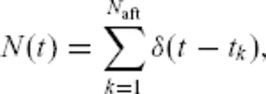
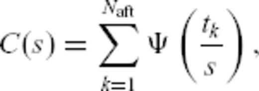
A2 Scaling function analysis of synthetic cases

We now apply the SFA to a variety of synthetic cases to demonstrate its efficiency. These synthetic tests will define benchmarks that will be used to interpret the results obtained for real catalogues. We use n_D = 0 to build the MSFs, except when explicitly mentioned.

A2.1 Omori law with a quadratic background term

While not directly similar to a real case, the first example illustrates the power of the SFA. The synthetic time-series that we choose to analyse is generated with the following formula

(A10)

over the interval [10⁻⁵;1] and is plotted in Fig. A3. This interval (where the time unit is 1 yr) is similar to those used for real time-series analysed in the text. The sampling rate is 10⁻⁵. It first exhibits a power-law decay followed by an explosive increase of N(t).

Figure A3.

Synthetic time-series N(t) = t^−0.8+ 10³t+ 10⁴t².

Open in new tabDownload slide

In order to analyse the time-series defined by (A10), we used four different MSFs, each function corresponding to a different value of n_B(0, 1, 2 or 3, the first three being represented in Fig. A1). The results are plotted in Fig. A4.

Figure A4.

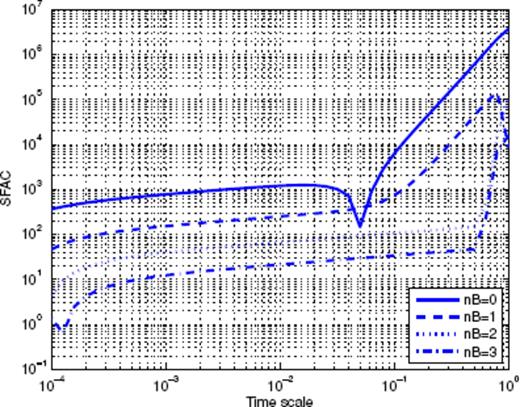
Scaling function analysis coefficient (SFAC) of the time-series shown in Fig. A3 as a function of the timescale s. Each curve corresponds to a given value of n_B used to build the corresponding mother scaling function (MSF).

Open in new tabDownload slide

According to the previous section and expression (A3), a linear behaviour in the log−log plot of Fig. A1 reveals an underlying power law with exponent 1 −p. For each curve, the power-law scaling is absent at the smallest scales which are comparable with the sampling rate, reflecting the signal digitization effect. The power-law scaling also breaks down at the largest scales, as N(t) is defined over a finite time range (a finite size effect), whereas the daughter scaling functions can take values significantly different from 0 over a larger range. For example, Fig. A1 shows that the chosen MSF remains significant in the interval [0;1.5], so that finite size effect will appear for timescales larger than about 2/3 in the SFA.

• (i)

  For n_B = 0, the MSF erases only the constant background contribution, which is anyway absent in the present example for N(t). As a consequence, a power-law scaling holds at small scales (up to about 10⁻²) with an exponent close to 0.2 (as expected from the prediction 1 −p for p = 0.8). Scaling then breaks down due to the existence of both the linear and quadratic contributions. At large scales, the exponent is close to 3, which means that the corresponding p-value is close to −2, which is exactly the signature of the quadratic term.

• (ii)

  For n_B = 1, the linear trend is erased, so that the power-law scaling now extends over a slightly larger range of timescales, with the same exponent, but the quadratic trend influence remains.

• (iii)

  For n_B = 2, the influence of the quadratic trend should be also erased, which is indeed the case as the power-law trend with exponent 0.2 now extends up to a scale s≈ 0.5.

• (iv)

  If we now increase n_B to 3, we see that the scaling range and exponent are the same, as there is indeed no contribution of higher degree to filter out (we obtain the same results using scaling functions with even larger n_B values).

Using this analysis, we are thus able to retrieve that the degree of the polynomial background term is n_B = 2, and that the Omori exponent is p = 1 − 0.2 = 0.8.

A2.2 Gamma law with constant background term

Fig. A5 shows a dashed-line plot of the gamma function

(A11)

It exhibits a power-law behaviour at small times, followed by an exponential roll-off at large times. This law could describe the time decay of swarms in volcanic areas, for example, with τ₀ being the characteristic duration of the swarm (here we took τ₀ = 10⁻³). The continuous line on the same figure shows the same function to which a constant background term B = 20 has been added. Note that this new time-series could very easily be mistaken for a pure Omori-law with a constant background. We performed a SFA of this last time-series, and Fig. A6 shows the obtained results using the same four scaling functions as above.

Figure A5.

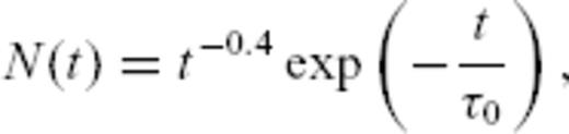
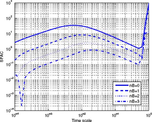
Gamma function (dashed line) defined by expression (A11) and Gamma function with an added constant background (continuous line).

Open in new tabDownload slide

Figure A6.

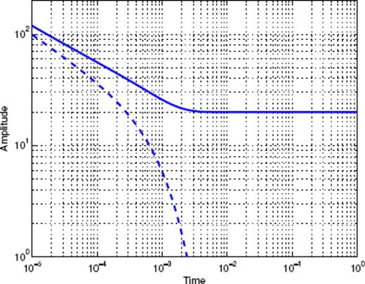
Scaling function analysis of the Gamma function with constant background term shown in Fig. A5. Each curve corresponds to a given value of n_B used to build the corresponding MSF.

Open in new tabDownload slide

As the only polynomial trend in N(t) is a constant term, all curves exhibit the same scaling behaviour, which results from two complementary effects. The first effect is that the gamma function can be described as an effective Omori-like power law with a tangent exponent p that continuously increases with time. Since the effective exponent is smaller than 1 at small times and larger than 1 at large times, the SFAC first increases and then decreases with timescale. The second effect is of a different nature. Fig. A5 illustrates that the Gamma function takes values significantly different from zero within a finite interval spanning roughly [0;10⁻²]. As the timescale increases, the associated SFAC will thus increase as the daughter scaling function progressively enters a kind of resonance with this finite-size feature. The maximum resonance is obtained when the scale of the daughter scaling function is of the order of 10⁻². Further increasing the timescale, the resonance amplitude decreases, leading to a decreasing SFAC. The interplay between those two effects leads to a reasonably well-defined maximum of the dependence of the SFAC as a function of the scale s, providing a rough estimate of τ₀. The drawback is that the left side of the power-law scaling behaviour in Fig. A6 is distorted and doesn't provide an accurate measure of p (in the present example, the measured p value is 0.2, compared with the true value p = 0.4). Overall, we conclude that the SFA clearly reveals the existence of a characteristic scale which precludes the existence of a genuine Omori scaling over the whole range of time. In this sense, the SFA provides a useful diagnostic. The final increase for the largest scales is due to the finite size of the interval over which the non-zero signal is defined.

A2.3 Mix of gamma law, Omori law and constant background term

The next synthetic example we wish to present is a sum of an Omori-like power law, a gamma law and a constant background term

(A12)

with τ₀ = 10⁻³. This function can describe the mixture of pure Omori-like sequences with swarm sequences in the presence of a constant background noise within the same data set. This function is plotted in Fig. A7 and displays a very complex time behaviour, that is sometimes observed in real time-series (see Fig. 1). When observing such a time-series, one generally tries to fit it with an Omori-law, considering that its fluctuations in log-log scale are just of statistical nature.

Using the same approach as before, Fig. A8 shows the results of the SFA on this function (A12). The obtained trend for small timescales is the same whatever the chosen value for n_B, and is compatible with a power law with an exponent close to 0.5 (corresponding to p = 0.5). The difference from the real exponent p = 0.4 is due to the same effects as in the case of the single gamma law discussed above. All curves then go through a maximum, and then decrease. This reveals the existence of a characteristic scale (which is τ₀ = 10⁻³ for expression A12). Then, for timescales larger than 10⁻¹, all curves increase again. This behaviour is due to the fact that, at such timescales, the gamma function is now negligible compared with the Omori-like contribution, and the SFAC exhibits a positive slope compatible with the true exponent p = 0.8 of the Omori law. As n_B increases, the maximum is shifted to larger and larger timescales, which implies that the positive slope to the right of this maximum which is associated with the Omori law can be observed only at larger and larger scales. As the timescales are limited by the time range of N(t), the slope corresponding to the Omori component can not always be measured with sufficient accuracy for the larger n_B values. However, we qualitatively find the same shape for all values of n_B.

A2.4 The modified Omori-Utsu law with constant background term

The modified Omori-Utsu law has been introduced as a convenient way to model the nearly constant seismicity rate after a large event at short timescales. We thus considered the following decay function

(A13)

which is shown in Fig. A9 for p = 1 and τ₀ = 10⁻⁴.

Figure A9.

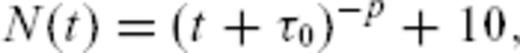
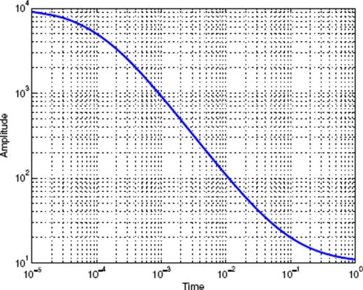
Modified Omori law defined by (A13) with a constant background term, for p = 1 and τ₀ = 10⁻⁴.

Open in new tabDownload slide

Results of the SFA are shown in Fig. A10. The SFACs first increase non-linearly (in log-log scales) up to a scale of about 10⁻¹, then behave as power laws with the associated exponent 1 −p = 0. Note that the transition from non-power law to power-law scaling is very smooth and thus offers a very small timescale range to estimate p, despite the fact that τ₀ is small.

Figure A10.

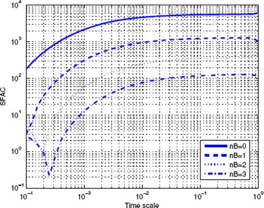
Scaling function analysis of the time-series shown in Fig. A9. Each curve corresponds to a given value of n_B used to build the corresponding MSF.

Open in new tabDownload slide

We also performed a SFA using n_B = 0 and different values of n_D(= 0, 5, 10, the number of orders of derivatives of Ψ that vanish at t = 0). Fig. A11 shows that, as n_D increases, the power-law scaling now holds for timescales larger than 10⁻², so that we can provide a more reliable determination of p.

Figure A11.

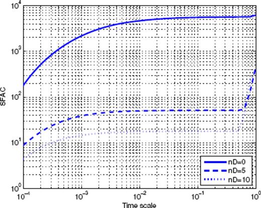
Scaling function analysis of the time-series shown in Fig. A9. Each curve corresponds to a given value of n_D used to build the corresponding MSF: n_D is the number of orders of derivatives of Ψ that vanish at t = 0.

Open in new tabDownload slide

A2.5 Piecewise power-law scaling

The next synthetic example we consider is the case of a piecewise power-law scaling with constant background,

(A14)

which is plotted in Fig. A12. This function has a characteristic timescale of 10⁻².

Figure A12.

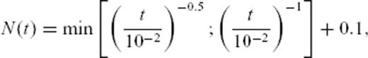
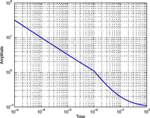
Piecewise power law with constant background term as defined by expression (A14).

Open in new tabDownload slide

The result of the SFA is plotted in Fig. A13. As the timescale increases, two power-law scaling regimes are revealed, separated by a smooth step at a timescale of about 2 × 10⁻², not too far from the built-in characteristic timescale of the process defined by expression (A14). The left part of the curves allows one to infer that the corresponding p-value is close to 0.5. The second right scaling range is not long enough to determine the scaling exponent with sufficient accuracy, but it gives however a rather good description of the change of exponent with scale/time.

Figure A13.

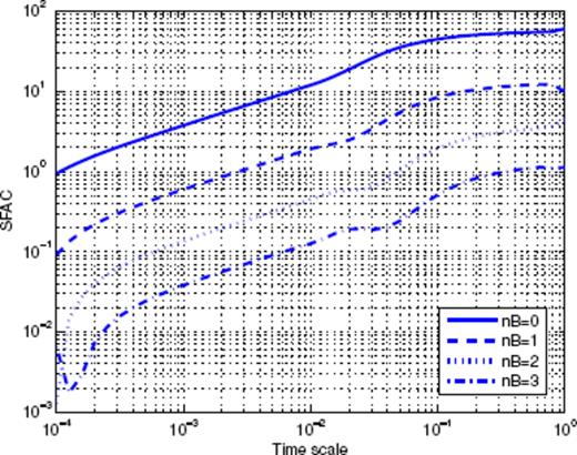
Scaling function analysis of the time-series shown in Fig. A12. Each curve corresponds to a given value of n_B used to build the corresponding MSF.

Open in new tabDownload slide

Now, setting n_B = 0 and using non-zero values for n_D, one can get a better picture of the complex scaling of N(t). Fig. A14 shows that increasing n_D sharpens the transition at timescale ≃10⁻², and that two different scaling ranges can clearly distinguished, over which the corresponding two values of the exponent p can be determined with high accuracy.

Figure A14.

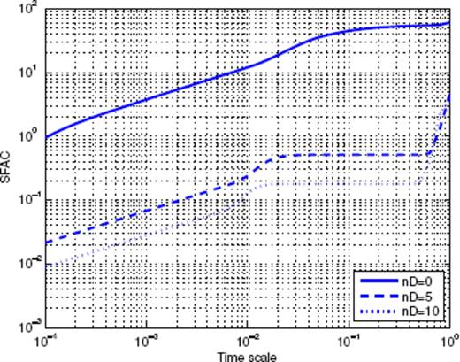
Scaling function analysis of the time-series shown in Fig. A12. Each curve corresponds to a given value of n_D used to build the corresponding MSF.

Open in new tabDownload slide

A2.6 Omori law with aftershock series from a previous event

This last example indeed illustrates a case that motivated the development of the SFA method. We use

(A15)

which is plotted in Fig. A15. The first term on the right-hand side stands for the aftershock sequence triggered by a main event at time t = 0. The second-term stands for the decay of the aftershock series triggered by a larger event that occurred 1 yr before. Note that this larger event triggered 100 times more aftershocks than the other one. The last term is the usual constant background term. One clearly sees that N(t) scales as a power law only for times lower than 10⁻³. At larger times, the power-law scaling is strongly distorted and slowed down by the occurrence of the previous event and the background term. Fig. A16 shows that we can retrieve the correct exponent p = 1 (so that 1 −p = 0) up to a timescale s = 10⁻¹ when n_B = 0. If n_B increases, the time interval over which power-law scaling holds widens, as the SFA method indeed progressively erases the contribution of the previous largest event. This shows that the potential contamination of aftershock time-series by previous larger events can reasonably be approximated by a polynomial function B(t) with low degree (2 or 3 at most).

Figure A15.

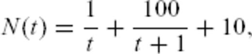
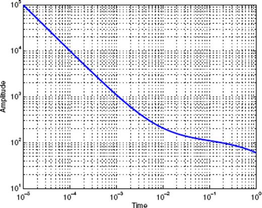
Omori-like decay mixed with constant background and an aftershock sequence triggered by a larger previous event.

Open in new tabDownload slide

Figure A16.

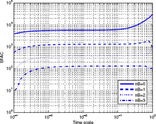
Scaling function analysis of the time-series shown in Fig. A15. Each curve corresponds to a given value of n_B used to build the corresponding MSF.

Open in new tabDownload slide