Tomographic resolution of ray and finite-frequency methods: A membrane-wave investigation Free

Summary

1 Introduction

Surface waves propagate within the outermost shells of the Earth. While earthquakes and seismic stations are non-uniformly distributed all over the globe, surface waves travel through remote regions where no stations can be placed. They sample the Earth's upper mantle relatively uniformly. Depending upon their frequency, surface waves are sensitive to different depth ranges in the mantle. For these reasons, observations of surface waves are a valuable source of information on the global structure of the Earth. Many studies have been conducted to measure phase anomalies of surface waves with respect to an a priori reference Earth (Laske 1995; Trampert & Woodhouse 1995, 1996, 2001; Laske & Masters 1996; Ekström et al. 1997; van Heijst & Woodhouse 1999). They lead to excellent databases of phase anomalies for surface waves with periods down to approximately 35 s. The measurement techniques differ in the details (Trampert & Woodhouse 2001), but share the main principle, which consists of filtering the seismograms around a period of interest within a narrow frequency band. The signal can also be decomposed into fundamental-mode and overtones as well as arrivals for multiple orbits. Synthetic seismograms are computed in a chosen, usually spherically symmetric, reference model. The phase anomalies are determined with respect to such synthetic seismograms by cross-correlation or other procedures (e.g. a downhill-simplex algorithm as in Ekström et al. 1997).

Once a number of source-station average dispersion curves have been measured, an inverse problem can be formulated, to determine the structure through which the surfaces waves travelled. Very large databases of phase-anomaly measurements are usually inverted for local phase velocities, leading to global phase-velocity distributions—which are, to first order, a linear combination of the underlying 3-D velocity structure. Before a seismic image is used for geodynamical interpretation or other applications, its resolution must be known. The resolving power of tomographic imaging is influenced by many factors, for example, by data coverage and measurement quality. It is often investigated by so-called checkerboard tests (Lévêque et al. 1993), solving for resolution radii (e.g. Trampert & Woodhouse 1996) or by examining the full resolution matrices (e.g. Boschi 2003; Boschi et al. 2007). All these studies are limited, in that the approximate theory used to formulate the inverse problem (ray theory) coincides with the theory used to compute synthetic data: inaccuracies in model resolutions resulting from inaccuracies in the approximate formulations of wave propagation cannot be estimated (Lévêque et al. 1993). In principle, one can overcome this problem by computing synthetic data with a completely numerical forward approach. Numerical forward simulations using different solution models can also identify model errors independent of their employed inversion methods, and thus objectively discriminate between the found solution models. Unfortunately, for a fully realistic 3-D earth model, this is extremely expensive (Qin et al. 2008), resulting in a very limited amount of available synthetic data.

Concerning the theories involved in the formulation of the inverse problem, global tomography has mostly relied on ray theory due to its intuitive physical interpretation and computational efficiency. When inverting for a phase-velocity model, ray theory requires the assumption that any perturbation of phase is due to a perturbation in phase velocity somewhere along the ray path of the considered phase. Especially for surface waves at longer periods, further away from the regime where ray theory is valid, this approximation might limit significantly tomographic resolution. Single scattering of surface waves causes phase-anomaly measurements made over a finite-frequency band to be sensitive to phase-velocity perturbations distributed over large areas on the globe, and not only on the ray (Woodhouse & Girnius 1982; Meier et al. 1997; Marquering et al. 1998; Spetzler et al. 2002; Zhou et al. 2004; Yoshizawa & Kennett 2005; Boschi 2006; Peter et al. 2007). These sensitivity areas, sometimes referred to as Born kernels (Marquering et al. 1998; Dahlen et al. 2000; Hung et al. 2000), are unique for every single measurement. In the presence of adequate data coverage, finite-frequency theory is expected potentially to reveal phase-velocity structures with spatial scalelengths smaller than the wavelength under consideration.

In the past, comparisons made between ray and finite-frequency theory have not decisively determined whether or not current formulations of finite-frequency theory improve the resolution of tomographic images. Zhou et al. (2005) showed an improvement when analytical finite-frequency theory was employed in 3-D inversions for seismic velocities. They also concluded that the 2-D problem of deriving phase-velocity maps was limited due to fact that it inherently uses ray-theoretical assumptions for the description of scattering, especially when simplifying its dependence upon depth. However, the statistical significance of such improvements remains to be determined. Concerning the inversion of phase-anomaly observations, Spetzler et al. (2002), Trampert & Spetzler (2006), Boschi (2006) and Peter et al. (2007) found that phase-anomaly observations for Love waves at intermediate to long periods were equally well inverted by rays and by Born kernels. The same can be deduced from Sieminski et al. (2004) at the regional scale, where a test with synthetically computed fundamental Rayleigh-wave data and a realistic distribution of events and stations suggested no improvement when using finite-frequency sensitivity kernels. On the other hand, Ritzwoller et al. (2002) inverted surface wave group-velocity measurements for group velocity models and found a clear difference at all periods between ray-theoretically and finite-frequency derived maps.

In this study, we compare different tomographic algorithms based on ray versus single-scattering finite-frequency theory. In Sections 2 and 3, we first consider the forward problem of predicting phase anomalies for a given phase-velocity model. In the first part of this study, we derive an asymptotic expression for membrane waves travelling on a sphere. This analytical expression can further be used to calculate waveforms for heterogeneous background models, once the ray path between source and station is found. We validate phase-anomaly predictions made by exact ray and finite-frequency theories, comparing them with numerical ‘membrane-wave’ results. In the second part of this study, we measure the accuracy of tomographic algorithms based on linearized ray-theory and finite-frequency tomography. The effects of scalelength, amplitude, noise and wavelength upon the imaging process are all specifically evaluated. To calculate synthetic data, we simplify the numerical approach by employing the membrane-wave method to simulate non-linear surface wave propagation effects for a laterally heterogeneous Earth. The synthetic databases are comparable in size to existing ones. We invert Love waves at intermediate to long periods with a realistic source-station distribution. Additionally, we investigate the effects of realistic noise in the data upon the inversion solutions and show to which extent they complicate comparisons between ray and finite-frequency theories.

2 Asymptotic Theory for Membrane Waves

To obtain the asymptotic, monochromatic waveforms of waves propagating on a heterogeneous membrane (Tanimoto 1990; Tape 2003; Peter et al. 2007), we first derive a travelling-wave expression of membrane waves for a homogeneous model. To then account for lateral heterogeneities, we calculate the phase and amplitude anomalies for a laterally heterogeneous phase-velocity distribution by a ray tracing algorithm. We use them to correct the homogeneous waveforms.

2.1 From standing waves to travelling waves

The idea is to start from a standing-wave representation of membrane waves and derive an analytical, asymptotic formulation in terms of travelling waves. Following the work of Gilbert (1976), we will conduct here a simplified treatment for waves propagating on a zero-thickness, spherical membrane (Tanimoto 1990). Motion on a membrane with wave velocity c is described by the equation

1

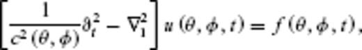
(e.g. Peter et al. 2007), where the displacement depends on colatitude , longitude φ and time t, while and denote time derivation and surface Laplacian on the sphere, respectively. We prescribe a forcing term

2

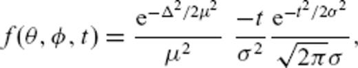
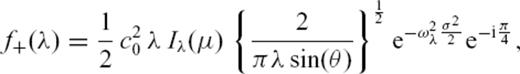
with arc-distance from the source . The source parameters σ and μ govern the characteristic frequency content of the source. An analytical solution is available for a constant velocity c₀ (Tape 2003, eq. 3.34):

3

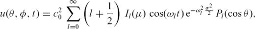
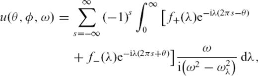
with P_l denoting the Legendre polynomials of degree l. The angular frequency at degrees is given by

4

for a given surface radius a. The integrals

5

can be evaluated numerically. Note that the waveform due to this initial source and given by eq. (3) is represented as a standing-wave summation.

2.1.1 Asymptotic approach and orbit separation

We rewrite eq. (3) with an asymptotic expression for the Legendre polynomials P_l (Gilbert 1976, eq. 9), valid for large degrees l. Additionally, we substitute and separate even from odd orbits, following the derivation of Ferreira (2005, appendix B1). Hence, we can rewrite

6

where

7

8

with * denoting a complex conjugate. The coefficients f₊ belong to waves for even orbits while the coefficients f₋ to those for odd orbits. From the standing-wave solution (6), applying Poisson's formula and transforming to frequency domain, we find the expression

9

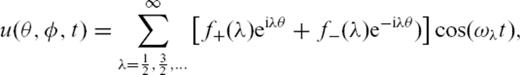
which has single poles at . Taking advantage of the general dispersion relation , which for the membrane-wave model becomes

10

we apply Cauchy's residue theorem to obtain

11

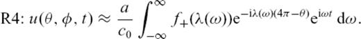
where terms are ignored. Finally, eq. (11) is Fourier-transformed back to time domain to find the travelling-wave solution

12

2.2 Travelling waves on a homogeneous membrane

The travelling-wave solutions for different orbits follow from the expression (12). For example, for odd orbits we set and use for the first, third, fifth and so on orbit. The corresponding expressions for the first and third orbits are

13

14

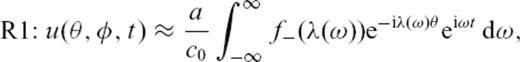
For even orbits, we set and use for the second, forth, sixth and so on orbits. The following expressions are for the second and fourth orbits:

15

16

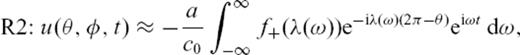
To plot the corresponding waveform solutions, we calculate the integrands of eqs (13) to (16) at each ω explicitly, and use a numerical integration to find . The Legendre polynomials P_l for non-integer values of the angular degree , with , are found numerically by spline interpolation. Similarly, the integrals , given by eq. (5), were interpolated by splines for non-integer values of the angular degree .

2.2.1 Waveform example

We choose an initial source-station pair with epicentral distance of about and compare the asymptotic solution against the numerical one. Fig. 1 shows the waveform for the fourth orbit obtained by the asymptotic approach of eq. (16) together with the numerical solution, calculated by finite-differences integration on a spherical membrane (Peter et al. 2007). Note that the numerical solution provides all orbits up to the end time of the computation. The asymptotic waveform has a slightly smaller amplitude at maximum displacement than the numerical one. The phase offset between the two is small. The agreement in this homogeneous case is good enough to proceed and obtain an asymptotic trace for a laterally heterogeneous model.

Figure 1.

Waveform solutions on a spherical membrane by the asymptotic approach for the fourth orbit (green), or calculated numerically (red) with the finite-differences membrane-wave model of Peter et al. (2007).

Open in new tabDownload slide

2.3 Ray theory on a heterogeneous membrane

The asymptotic approach provides us with a waveform for a homogeneous membrane-wave model. To extend the treatment of Section 2.2 to the heterogeneous case, we first use the laws of optics to determine the ray path travelled by a wave (Woodhouse & Wong 1986; Boschi & Woodhouse 2006), then compute the phase by integration along such a ray.

2.3.1 Ray tracing

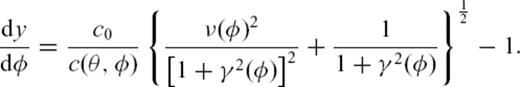
To calculate the phase for a heterogeneous background model

17

with local phase velocities , we need to compute the corresponding ray between the seismic source and a receiver station, a problem treated by Woodhouse & Wong (1986) for the sphere. For brevity, we just give the two equations which relate to our case here. We simultaneously solve for and in eqs (33) and (38) of Woodhouse & Wong (1986):

18

19

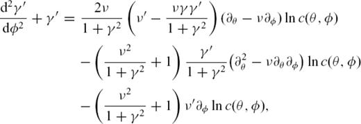
where and ′ denotes differentiation with respect to the initial value of ν, at constant φ. The boundary conditions are and . It should be clear that in this formulation the colatitude is a function of longitude φ, describing the ray.

2.3.2 Ray-theoretical traveltime anomalies

Let us rotate the reference frame such that source and receiver are located on the equator. becomes the epicentral distance between source and receiver. For a homogeneous reference model, the phase can be written as

20

where a is the Earth's radius and c₀ the constant phase velocity for the reference model. The phase anomaly is defined as the difference in phase from that in the reference model, that is (Woodhouse & Wong 1986, eq. 42)

21

22

Note that the phase anomaly is calculated for a single frequency at a certain reference period .

We use local phase velocities which are derived from maps of relative phase-velocity perturbations at given taken from Trampert & Woodhouse (1995). We can define

23

so that

24

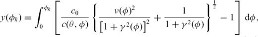
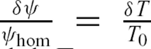This can be solved simultaneously with the other eqs (18) and (19) from above. We prefer working with traveltime anomalies, thus we make use of the identity between relative phase anomalies and relative traveltime anomalies , where T₀ denotes the traveltime for the reference model. From eq. (20), we find

25

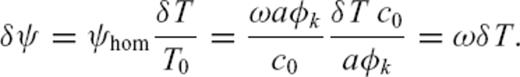
3 Comparison of Different Approaches to the Forward Problem

To compare predictions of traveltime anomalies, we model an array of 38 receivers located at about 90° epicentral distance from one source at 0°N, 0°E. The heterogeneous phase-velocity model for Love waves at about 150 s period is taken from Trampert & Woodhouse (1995). We conduct a series of independent experiments, where we expand the model up to degrees 4, 8, 12 or 20, respectively. The setup is similar to the one used in Tape (2003). For each source-station pair, we consider arrivals up to the fourth orbit, thus at least 152 prediction values are compared for each of the four different models. The numerically derived values, which are recalculated for each model with different degrees of complexity, can be seen as the ‘true’ values, which the predicted ones should match in an ideal case.

3.1 Evaluation of ray theory

We first compare the ray-theoretical predictions of traveltime anomalies against numerically calculated traveltime anomalies. A reference trace for the homogeneous model and a second trace for the heterogeneous model are computed numerically with the finite-differences approach of Peter et al. (2007). We bandpass-filter the two numerical traces around an angular frequency ω, for which we have also determined ray-theoretical traveltime anomalies according to eq. (25). The ray-theoretical predictions are calculated for both exact rays as are given by eqs (18) and (19), and great-circle rays corresponding to the first-order approximation. The bandpass-filter uses a half-bandwidth of 2.5 mHz around the centre frequency ω. Following Ekström et al. (1997), we then determine the corresponding numerical traveltime anomaly by a non-linear downhill-simplex algorithm (Nelder & Mead 1965). We checked this algorithm against a cross-correlation measurement technique and found almost identical results for the phase anomalies.

Fig. 2 compares the traveltime anomalies calculated by eq. (25) for exact and linear ray theory with the corresponding measurements derived from the numerical simulation. Values on the diagonal correspond to perfect agreement. We see that ray theory predicts the first-orbit anomalies accurately; for higher orbits (shown with different symbols), the values are more scattered around the diagonal, particularly for models with energy at increasingly high harmonic degrees (compare Fig. 2a with Figs 2b–d). In general, the plots of Fig. 2 are in agreement with the results of Tape (2003). Particularly large differences between the ray-theoretical prediction and the ground-truth value for higher orbits and expansions are observed when multiple ray paths between source and receiver location exist (in such cases, we plot in Fig. 2 the traveltime anomaly calculated from the phase-anomaly associated with the first ray found by our ray tracing algorithm).

Figure 2.

Ray-theoretical predictions of traveltime anomalies (RAY) using exact rays (exact) given by eqs (18) and (19) and linear/great-circle rays (linear) are plotted in blue and green, respectively, against the numerically calculated, ground-truth ones (numerical traveltime anomaly) for 38 source-station pairs with about 90° epicentral distance. The source is located at 0°N/0°E. The phase-velocity map is taken from Trampert & Woodhouse (1995) filtered to maximum harmonic degrees (a) 4, (b) 8, (c) 12 and (d) 20. predictions for the first orbit are plotted as squares, second orbit as diamonds, third orbit as triangles and fourth orbit as circles. The grey shaded area around the diagonal indicates the standard deviation of 5.7 s for traveltime measurement errors estimated by Ekström et al. (1997) for Love waves at 150 s period.

Open in new tabDownload slide

As expected, predictions from linearized ray-theory using only great-circle rays degrade faster than predictions from exact ray theory, particularly for higher-orbits and higher-degree heterogeneity. However, for 150 s Love waves at least, differences between exact and linear predictions for first- (and second) orbit arrivals are smaller than the phase-anomaly measurement error as estimated by Ekström et al. (1997). Interestingly, traveltimes for both linearized and exact rays appear to be slightly biased towards earlier (negative) traveltime anomalies in our study. This is explained by the distribution of our sources and stations, which for the 150 s Love-wave phase-velocity map of Trampert & Woodhouse (1995) results in waves travelling mostly through faster-than-average regions.

3.2 Evaluation of finite-frequency theory

We also consider the traveltime anomalies predicted on the basis of the finite-frequency kernels derived by the single-scattering approximation, specifically the numerical kernels 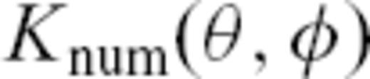from Peter et al. (2007). These kernels were derived by the adjoint method (Tromp et al. 2005, and references therein) and computed for both homogeneous and heterogeneous background models. We calculate the corresponding traveltime anomaly by integrating

26

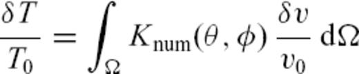
over the surface Ω of the membrane, and multiplying with the reference traveltime T₀ of the homogeneous case. denotes relative phase-velocity perturbations in the model of Trampert & Woodhouse (1995) expanded up to degrees 4, 8, 12 or 20. Fig. 3 compares the traveltime anomalies calculated this way, with the corresponding ground-truth ones. The kernels are computed for every orbit separately. An example of the numerical kernels based on the homogeneous background model for a particular source-station pair for all four orbits is given in Fig. 4. Note that the shape of the kernels is strongly affected by the filtering at 150 s period (corresponding to the measurement technique) with a half-bandwidth of 2.5 mHz.

Figure 3.

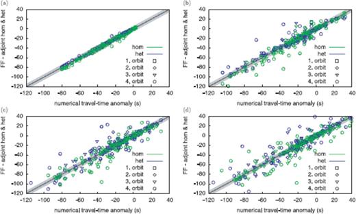
Finite-frequency predictions of traveltime anomalies (FF) calculated via eq. (26) are plotted versus the numerically calculated ones (numerical traveltime anomaly), employing sensitivity kernels computed for both homogeneous (hom) and the corresponding heterogeneous (het) background phase-velocity maps. Source, stations and earth model are the same as in Fig. 2. The phase-velocity map from Trampert & Woodhouse (1995) is filtered to maximum harmonic degrees (a) 4, (b) 8, (c) 12 and (d) 20. predictions for the first orbit are plotted as squares, second orbit as diamonds, third orbit as triangles and fourth orbit as circles.

Open in new tabDownload slide

Figure 4.

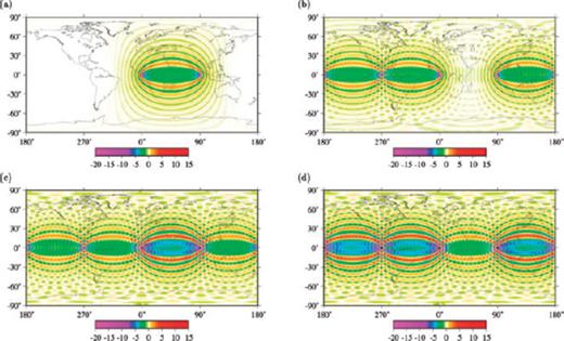
Example of numerical sensitivity kernels (Peter et al. 2007), based on the adjoint method, used for the predictions of traveltime anomalies (FF, hom) in Fig. 3 for the source located at 0°N/0°E and a receiver at 0°N/90°E. Plotted are the relative traveltime kernels for the (a) first, (b) second, (c) third and (d) fourth orbits.

Open in new tabDownload slide

Analysing the scatter in Figs 2 and 3, we find that finite-frequency predictions are more accurate than the ray-theoretical ones of Fig. 2 only for the first orbit. As a quantitative measure of scatter, we used a linear regression to calculate the rms of the residuals shown in Table 1, which for linear ray-theoretical predictions of first-orbit arrivals range between 0.1 and 1.1 s for the background phase-velocity map filtered to degrees 4, 8, 12 and 20 (Figs 2a–d). The corresponding rms ranges for residuals of the finite-frequency predictions using homogeneous background kernels of first-orbit arrivals shown in Figs 3(a)–(d) are between 0.1 and 0.6 s. At higher orbits, the situation is reversed, with exact ray theory predicting ground-truth traveltime anomalies more accurately than the finite-frequency kernels. We tested also predictions from analytical kernels for the first and second orbit, calculated as in Spetzler et al. (2002). Their analytical kernels are computed with ray theory, like the ones from Zhou et al. (2004) or Ritzwoller et al. (2002). The scatterplot results shown in Figs 5(a)–(d) are analogous to those found from numerical kernels. The rms residuals for numerical (heterogeneous and homogeneous) and analytical finite-frequency predictions shown in Table 1 follow in general the values associated with linearized ray theory. Finite-frequency kernels suffer, especially for higher orbits, from their inherent linearity. A similar effect has been noted in attempts to compute higher-orbit waveforms by the Born approximation (Capdeville 2005, see fig. 8), demonstrating that non-linear effects become significant for longer travel distances.

Table 1.

rms values of the residuals for a linear regression through the predicted traveltimes anomalies versus the ‘ground-truth’ numerical ones shown in Figs 2, 3 and 5.

Open in new tabDownload slide

Figure 5.

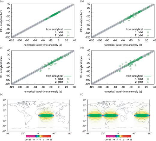
Finite-frequency predictions of traveltime anomalies using analytical sensitivity kernels for minor- and major-arcs as described by Spetzler et al. (2002). Source, stations and earth model are the same as in Fig. 3. The phase-velocity map from Trampert & Woodhouse (1995) is filtered to maximum harmonic degrees (a) 4, (b) 8, (c) 12 and (d) 20. predictions are shown for the first (squares) and second orbits (diamonds). An example, similar to Fig. 4, of the analytical sensitivity kernels for the source located at 0°N/0°E and a receiver at 0°N/90°E is given for the (e) first and (f) second orbits.

Open in new tabDownload slide

In general, the accuracy of prediction depends upon the ratio of the scalelength Λ of heterogeneities to the width W of the first Fresnel zone. Baig et al. (2003) and Dahlen (2004) define a dimensionless ‘doughnut-hole’ parameter D valid for their 3-D sensitivity kernels in a cartesian box model

27

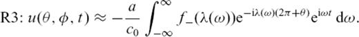
where L denotes the travelled distance and λ the wavelength. Spetzler & Snieder (2001) adapted the width to spherical geometry, limited to the 2-D (surface wave phase velocity) case, thus

28

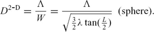
Theoretically, it is assumed that for , ray-theoretical predictions would become perfectly accurate.

For wave propagation in a weakly heterogeneous, 3-D cartesian box, Baig et al. (2003) found that finite-frequency predictions are accurate for , and ray-theoretical ones only for . Yang & Hung (2005) found that for analytical finite-frequency sensitivity kernels, in a similar 3-D case, traveltime predictions are only accurate for weakly heterogeneous media with perturbations ≤ 3 per cent. Their Fig. 2 shows that ‘Born’ theory predictions are less accurate than those of exact (general) ray theory for . 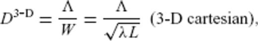In our heterogeneous models, phase-velocity perturbations can amount to about ±6 per cent, and depending upon the maximum degree of harmonic expansion, Λ varies between 1953 and 8896 km, with corresponding doughnut-hole parameters (for our first-orbit kernels with epicentral distances). Only for first-orbit arrivals, we found finite-frequency kernels to perform similarly to or better than exact ray theory as a solution to the forward problem. Finite-frequency predictions otherwise follow the same error trend as linearized ray-theory.

3.3 Multiple ray path example

For higher-orbit arrivals and higher maximum degree phase-velocity maps, there are cases where multiple rays are found (see also Tape 2003; Ferreira & Woodhouse 2007). A reference case shown in Fig. 6 is chosen here for a source-station pair such that we obtain three ray paths, for the fourth orbit, which arrive at the same station location (source at equator 0°N/0°W, station at about 25°N/90°W). Rays are traced, and phase calculated in the 150 s Love-wave phase-velocity map of Trampert & Woodhouse (1995), with a spherical harmonics expansion up to degree 10. The considered case is the only multipathing occurrence found for this phase-velocity map and maximum harmonic degree, among 38 investigated source-station pairs with about 90° epicentral distance. If the model is filtered to lower harmonic degree, no multiple ray paths are found for the same source-station pairs; at higher harmonic degrees, multipathing becomes increasingly frequent.

Figure 6.

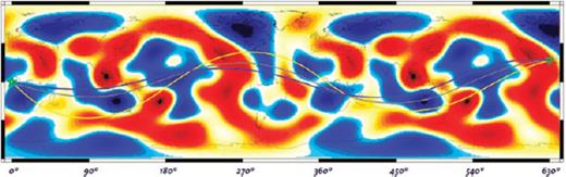
Multiple ray paths for a reference case with the fourth-orbit arrival in a heterogeneous background phase-velocity distribution (Trampert & Woodhouse 1995). All three rays solve the same ray tracing equations from Woodhouse & Wong (1986) leading to different phase- and amplitude-anomaly predictions shown in Table 2.

Open in new tabDownload slide

The ray tracing algorithm calculates for each ray, denoted by i = 1, 2, 3, the corresponding phase anomaly , which is further divided by the angular frequency to obtain the corresponding traveltime anomaly for monochromatic waves with a period of about 150 s. To obtain the waveform, the amplitude anomaly for each ray is considered as well. The cumulative travelled epicentral distance from source to receiver is 630°. The ray-theoretical predicted values are applied to the monochromatic trace obtained by filtering first the asymptotic waveform for the fourth orbit (see Section 2.2). We further corrected the traveltime and amplitude of the monochromatic waveform for all three rays separately by the predicted traveltime anomaly and amplitude anomaly A_i to obtain three single waveforms

29

Finally, all three waveforms are summed up to obtain the resulting one

30

Note that is now valid for the heterogeneous model.

Eq. (30) is also implemented via the harmonic addition theorem, expressing the sum of n harmonic waves as

31

where

32

33

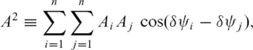
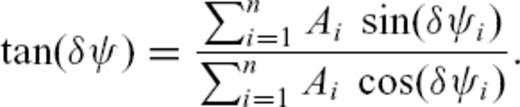
Hence, the resulting phase anomaly , resp. traveltime anomaly , and amplitude anomaly A of as defined by eq. (30) can be calculated directly from the single predictions and A_i. We compare all values with the traveltime and amplitude anomaly obtained by the numerical algorithm in Table 2.

Table 2.

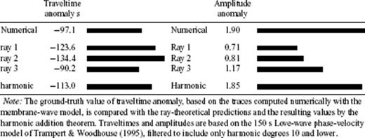
Example of multipathing, with three fourth-orbit rays joining source and receiver.

Open in new tabDownload slide

We observed that the resulting, asymptotic waveform, given by eq. (30), was shifted by about 17 s and exhibited a slightly larger amplitude of about 5 per cent with respect to the numerical, ground-truth trace. Note that the discrepancy of these observed anomalies to the analytical, harmonic values from Table 2 might be found in the finite bandwidth of the single traces used for the summed waveforms of eq. (30), while the analytical values are valid only for monochromatic waves. Still, the traveltime anomaly of the resulting trace is closer to the numerical, ground-truth prediction than the single predictions for the second and third rays, but worse than the prediction of the first ray. It is therefore crucial to find all rays to properly account for the predicted anomalies.

Our study differs with respect to the work on synthetic seismograms of a more realistic case by Wang & Dahlen (1994, see fig. 21). We consider only the monochromatic (or very narrowly filtered) waveform for an analytical source, instead of an integration over a complete frequency range. Such an integration becomes more expensive as for each frequency the corresponding, ray-theoretical phase and amplitude anomalies must be found first. Additionally, we investigated especially a multiple ray path example where Wang & Dahlen (1994) only consider single ray examples. A more systematic investigation of multipathing effects as done here could in principle be conducted with the membrane-wave model (Tanimoto 1990; Tape 2003; Peter et al. 2007).

4 Comparison of Different Approaches to the Inverse Problem

To compare the performance of different tomographic methods in different scenarios, we construct a number of independent databases of ground-truth, numerically computed phase anomalies of 150 s Love waves, and invert them either by a ray-theoretical or a finite-frequency algorithm. Differences in the solution maps can then be ascribed to the effects of different theoretical descriptions of seismic wave propagation. Databases are derived from three ‘checkerboard’ phase-velocity maps of different spatial frequency, as well as from the model of Trampert & Woodhouse (1996). We also experiment with the amplitude of ‘input’ anomalies, and with realistic random noise added to the synthetics. We invert each ground-truth data set on a grid of approximately equal-area pixels, of extent at the equator. Linearized ray-theory and numerical finite-frequency kernels (computed on a homogeneous background phase-velocity map by Peter et al. 2007) are used independently to construct the corresponding matrices relating phase-velocity perturbations to the data.

In both cases, a least-squares algorithm (Paige & Saunders 1982; implemented as in Boschi 2006) finds the phase-velocity solution to the inverse problem, with only roughness-damping and no norm-damping applied. We repeat the inversions with different roughness-damping coefficients (Boschi 2006; Boschi et al. 2006; Peter et al. 2007) and visualize the ‘L-curves’, where the misfit to the data is plotted versus the normalized model roughness (as defined by Boschi 2006) on a log-log scale. As explained by Boschi (2006) in his section 4 and fig. 3, if different formulations of the inverse problem are applied, equal numerical values of the damping parameter do not lead to equally regularized solutions from the different approaches: we therefore need to (1) compare entire families of solutions and/or (2) identify an equivalent criterion to select the damping parameter values in the two formulations. (1) We systematically visualize how solution models change as a function of damping parameter value, merging in a single animation the sequence of solutions corresponding to a given surface wave mode and a given theoretical formulation. We provide the animations on line at. From the comparison of ray-theory versus finite-frequency animations, it is apparent that the latter is performing better than the former: of the ray-theory results, even the most similar to the input model are visibly less well correlated with it than the finite-frequency ones. (2) We choose the criterion of maximum curvature of the L-curve (Hansen 1992; Hansen & O'Leary 1993) to identify equivalently regularized solutions from ray-theory and finite-frequency inversions. Given the impossibility of including animated images in a traditional publication, in the following we limit ourselves to comparing specific solutions resulting from the maximum curvature criterion.

4.1 Data coverage

We employ the same source-station pairs as in the database of Ekström et al. (1997), updated as described by Boschi & Ekström (2002), for minor-arc Love waves at 150 s period. For each source-station pair, we construct a synthetic measurement by cross-correlation between the trace obtained for a homogeneous background model, and the trace calculated for a corresponding laterally heterogeneous input model. The number of synthetic measurements (∼10⁴) is therefore equal to the number of observations in the real data set at this period. Fig. 7 shows the great-circle rays for all measurements with the chosen source-station distribution. The data coverage defined by the number of rays passing through each single pixel of the inversion grid coincides with that of Peter et al. (2007, fig. 12). Regions with the highest number of ray counts are distributed over Asia and North America. The Southern Hemisphere in general has relatively poor data coverage.

Figure 7.

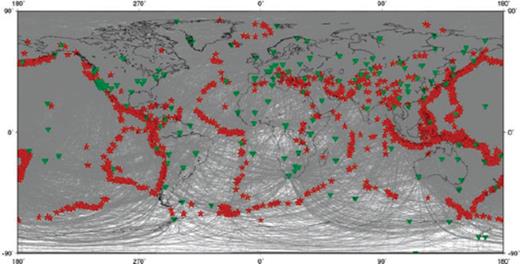
The synthetic data sets use the global distribution of sources (red stars) and stations (green triangles) taken from Ekström et al. (1997) for Love waves at 150 s periods. They include 16 624 measurements. For each measurement, the great-circle ray is plotted between the corresponding source and station.

Open in new tabDownload slide

4.2 Scalelength test

We compare the inversions of synthetic data computed from assumed velocity distributions of different spatial frequencies, each coinciding with a single spherical harmonic function (similar to a global checkerboard). To illustrate the effect of different scalelengths of heterogeneities upon the performance of the inverse method, we can either (1) change the spatial extent of the perturbations in the input models or (2) consider smaller wavelengths/wave periods.

Figs 8 and 9 show the results of experiment (1), Fig. 10 those of experiment (2) respectively. The L-curves (defined as in Hansen 2001, eqs 12 and 13) for ray-theoretical and finite-frequency inversions, with different strengths of roughness damping, are shown in Fig. 8. For each L-curve, we calculate its curvature and select the solution corresponding to the maximum curvature as our preferred solution. In our synthetic test, we can calculate, for each solution, the rms difference between solution and input phase-velocity models. As can be seen in Fig. 8, the curvature maxima for finite-frequency inversions are close but not necessarily identical to the solutions with minimal rms error. The same is true in the ray-theory case. Still, we consider solutions found by this criterion to be sufficiently close to the optimal ones. Importantly, damping parameters corresponding to optimal solutions are different in the ray-theoretical versus finite-frequency cases. In the rest of this study, we will adhere to this maximum-curvature criterion to find equivalently regularized solutions in ray-theoretical and finite-frequency inversions.

Figure 8.

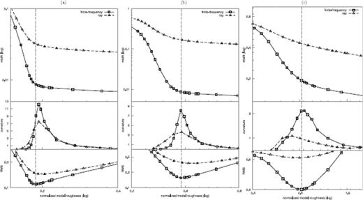
L-curves (misfit versus normalized model roughness) for the suites of ray-theoretical (triangles) and finite-frequency (squares) synthetic inversions described in Section 4.2. Plots from left- to right-hand side correspond to different input models, namely: (a) a single spherical harmonic of degree l = 9 and order m = 5, (b) l = 13 and m = 7 and (c) l = 20 and m = 10. Top: L-curves shown on a log-log scale. Bottom: curvature of the L-curves, and rms of the difference between input and output models. Vertical dashed lines mark finite-frequency solutions corresponding to the minimum difference between input and output: importantly, they are close to the points of maximum curvature on the L-curve.

Open in new tabDownload slide

Figure 9.

Inversions for Love waves at 150 s period and input models of 2 per cent perturbations and different scalelengths of heterogeneities: (a) checkerboard defined as a single spherical harmonic of degree l = 9 and order m = 5, (b) checkerboard with l = 13 and m = 7 and (c) checkerboard with l = 20 and m = 10. The input models are shown in the left-hand column, solutions corresponding to the maximum curvature in Fig. 8 for the ray-theoretical inversions in the middle and finite-frequency inversions on the right-hand column.

Open in new tabDownload slide

Figure 10.

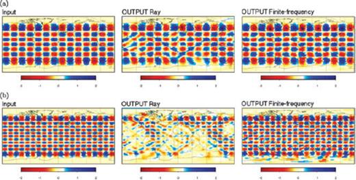
Inversions for Love waves at 100 s period and input models of 2 per cent perturbations and different scalelengths of heterogeneities: (a) checkerboard with spherical harmonic degree l = 13 and m = 7 and (b) checkerboard with l = 20 and m = 10. The input models are shown in the left-hand column, solutions of the ray-theoretical inversions in the middle and finite-frequency inversions on the right-hand column.

Open in new tabDownload slide

Fig. 8 shows the solution models that correspond to the maximum curvatures of the L-curves. The selected ray-theoretically derived solutions start differing from finite-frequency solutions for the higher-degree input models. The lengthscale of the perturbations for the chosen input models vary in a range of ∼2000–4000 km, that is, about three to six times the wavelength under consideration. Fig. 10 follows the idea (2) and changes the wave period down to 100 s to derive the synthetic data sets for the two higher-degree checkerboards of the previous example. In this case, at the highest-degree model, the lengthscale of perturbations is about four times the wavelength. Especially for regions with good data coverage, the inversions can retrieve the input model fairly accurately.

From a comparison of Fig. 9(a) with Fig. 9(b) or (c), or of Fig. 10(a) with Fig. 10(b), we infer that finite-frequency methods, applied to minor-arc phase-velocity data at the periods under consideration, perform significantly better at smaller scalelengths of heterogeneity than ray-theoretical methods. Differences between ray-theoretical and finite-frequency solutions are small for low-degree ‘input’ models (<10: Fig. 9a), but start to become significant for higher degrees (≥ 13: Figs 9b, c and 10b). Considering shorter wavelengths, this effect shifts to higher spherical harmonic degrees (compare Fig. 9b with Fig. 10a). The finite-frequency solutions clearly retrieve the input structures with higher accuracy. Differences are most prominent in regions with lower data coverage (oceans, Southern Hemisphere), where ray theory is systematically less accurate. As a general rule, in this ideal case without any noise in the data, finite-frequency solutions achieve a much better datafit than ray-theoretical ones.

4.3 Noise test

The goal here is to investigate the effect of measurement errors on the tomographic images. Adding realistic noise to a synthetic database is difficult, because there can be sources of systematic errors, which are not known a priori, in the real databases. Ekström et al. (1997) estimate the quality of their observations by comparing measurements from pairs of nearby source-station pairs. In this, they are able to derive a Gaussian distribution of possible errors of the data set. The standard deviation of this Gaussian distribution is then an estimate of the accuracy of the measurement technique. We add Gaussian random noise to the synthetic data. The standard deviation has the same size as that found by Ekström et al. (1997) as described above, for the same wave period. This is about 5.7 s in terms of traveltime shift. The error in the synthetic data set is also checked by the same searching algorithm of pairs of source-station pairs that are within a 3° radius from source and receiver location.

We show in Fig. 11 the results of inverting the noise-added, ground-truth database constructed from the degree 13 (Fig. 11a) and degree 20 (Fig. 11b) checkerboards (left-hand panels), using the ray-theory (middle panels) and finite-frequency-theory based (right-hand panels) inverse algorithms. By comparing with the optimal rms solutions for this case here, we noticed that the maximum curvature criterion leads to solutions that are slightly overdamped. In contrast to Figs 9(b) and (c), the statistical noise degrades the solutions and diminishes the differences between the two approaches in question. This is in agreement with what suggested Sieminski et al. (2004). Still, even in the presence of noise, our solutions from finite-frequency inversions are somewhat closer to input models than those found from ray-theory ones.

Figure 11.

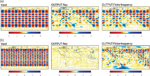
Using statistical noise in the synthetic data set, solutions for Love waves at 150 s period and an input model of 2 per cent perturbations are shown: (a) with a checkerboard with l = 13 and m = 7 and (b) with a checkerboard with l = 20 and m = 10. The input models are shown in the left-hand column, solutions of the ray-theoretical inversions in the middle and finite-frequency inversions on the right-hand column.

Open in new tabDownload slide

These results are somewhat different from those obtained for global scale inversions by Zhou et al. (2005, see fig. 19). There are, however, a few important differences between their study and ours: (1) unlike Zhou et al. (2005), we construct the synthetic database by means of a non-linearized numerical method, so that the accuracy of the synthetics is not hindered by the same approximations used in the inversion, as is the case in classical checkerboard tests conducted by Zhou et al. (2005). (2) While Zhou et al. (2005) adds Gaussian-distributed, random noise with an rms error of about 50 per cent of the ‘structural signal’, we apply the same kind of statistical noise but with the same standard deviation as found in the real data set of Ekström et al. (1997). The amplitude of noise is therefore different. Additionally, the effects of noise strongly depend on the data coverage of the data set, which is also different between the two studies. (3) Zhou et al. (2005) calculate analytical sensitivity kernels based upon a far-field approximation, while our kernels are computed strictly numerically. We also use a different coarseness of the inverse grid, which leads to different resolution of the kernels actually used by the inverse algorithm. As we use a slightly finer parametrization, our kernels will be represented in more detail thus exhibiting a bigger difference to rays, which itself can be assumed to lead to bigger differences in the inverse solutions found between the two theories.

4.4 Amplitude test

Both ray and single-scattering finite-frequency theories are linearized theories, whose performance is contingent on the extent and amplitude of perturbations with respect to a reference model, that is they fail when applied to (very) rough media. We next explore the specific non-linear effects of the amplitude of Earth's structure heterogeneities in an example case with amplitude perturbations as high as ±10 per cent. The input model pattern is a checkerboard, coinciding with the spherical harmonic function of degree 9 and order 5 as in the previous Section 4.2. The synthetic database is then constructed for Love waves at 150 s period without any statistical noise.

Images resulting from the inversion of the corresponding synthetic data set are shown in Fig. 12(a). Comparing them with the solutions plotted in Fig. 9(a), we see that both theories suffer from their inherent linearization. The power spectra of the ray-theoretical solution in Fig. 12(b) and of the finite-frequency solution in 12(c) both reveal the initial power spectrum of the 10 per cent checkerboard input model with a strong peak at spherical harmonic degree 9, the finite-frequency solution achieving a slightly higher peak. Both power spectra show further aliasing of energy towards surrounding harmonic degrees. Note that non-linear effects are not only degrading the performance of both inverse methods, but they also tend to affect the stability of the solutions, so that maximum curvature of the L-curve is achieved for values of the damping parameters higher than in the experiments described above.

Figure 12.

Influence of large amplitude of heterogeneities. Solutions are shown for Love waves at 150 s period and an input model of (a) 10 per cent perturbations with a checkerboard with l = 9 and m = 5. On the left-hand side, the input model is shown, while in the middle and on the right-hand side the ray-theoretical and finite-frequency solutions, respectively, are plotted. The power spectrum up to spherical harmonic degree 25 is shown of the ray-theoretical solution image in (b) as red bars, the corresponding one of the finite-frequency solution image in (c), both plotted against the initial power spectrum of the input model (black box).

Open in new tabDownload slide

To overcome such limitations, a non-linear solution could be found iteratively, using the solution of a previous inversion as a new starting model to reconstruct the matrices for a new inversion. We tested this approach in the finite-frequency case, computing all sensitivity kernels again in the new starting model (Peter et al. 2007). Even after three iterations, the solution (not shown here) did not improve significantly. Starting each iteration with a highly damped model (and, consequently, a relatively poor datafit) increases the total number of iterations needed to find a sufficiently good result. On the other hand, starting with a rougher model like the output models of Fig. 12, the solution is perturbed very little at each iteration. This suggests that the inverse scheme might be trapped at a local minimum of the misfit function.

4.5 Realistic input model test

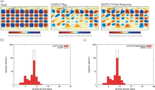
While the checkerboard test provides a useful measure of resolution, it is still of interest to determine the way in which imperfect resolution reflects itself on the tomographic inversion of a realistic phase-velocity distribution. We choose as input model the phase-velocity map originally derived by Trampert & Woodhouse (1996) for Love waves at 150 s period. The source-station distribution of Trampert & Woodhouse (1996) differs from the distribution assumed here (Section 4.1). We conducted ∼10⁴ synthetic measurements based on the source-station distribution of Ekström et al. (1997) and added statistical noise as described in Section 4.3, to obtain the synthetic database. Fig. 13(a) shows the preferred solutions for the ray-theoretical and finite-frequency inversion methods. The power spectra of both solutions are plotted against the power spectrum of the input model in Figs 13(b) and (c); the power spectrum of both the ray-theoretical and finite-frequency inversion results is slightly overpredicting the lowest harmonic degrees while losing energy at higher degrees (>8).

Figure 13.

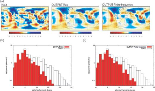
Realistic input model TW96 solved for Love waves at 150 s period. (a) The input model is shown on the left-hand side, the ray-theoretical inversion in the middle and the finite-frequency inversion solution on the right-hand side. The corresponding power spectra up to spherical harmonic degree 25 of (b) the ray-theoretical solution image (red bars) and (c) the finite-frequency solution image (red bars) are plotted against the initial power spectrum of the input model (black boxes).

Open in new tabDownload slide

As explained above, solutions compared in Fig. 13 were selected after an L-curve analysis with the criterion of maximum curvature proposed by Hansen (1992) and Hansen & O'Leary (1993). Those authors concluded that the misfit to the data is an effect of both regularization and measurement errors, and that the ‘corner’ of the L-curve corresponds to a balance between the two. They also showed that the maximum-curvature solution corresponds to the solution also found by the quasi-optimality criterion as well as the generalized cross-correlation, but that especially in presence of noisy data the L-curve criterion remains more stable. We observe that employing this criterion slightly overregularizes the solution in presence of noise. As a result, Fig. 13 shows smooth ray-theoretical and finite-frequency solutions. This might somewhat reduce the discrepancy between the results of the two approaches.

5 Conclusions

Using the asymptotic approach, we derived an analytical description for the propagation of elastic waves on a zero-thickness membrane in terms of travelling waves, consistent with the more general treatments of Gilbert (1976) and Ferreira (2005). We used this formulation of ray theory on a membrane in a comparison to the forward predictions of finite-frequency kernels (analytical and numerical: see Peter et al. 2007), and a ground-truth database of numerical, membrane-wave synthetics. Our work extends the investigations made for 3-D sensitivity kernels within 3-D cartesian boxes (Baig et al. 2003; Baig & Dahlen 2004; Dahlen 2004; Yang & Hung 2005) to a 2-D spherical geometry. We further employed finite-frequency sensitivity kernels for higher orbits. While predictions made by finite-frequency theory for first-orbit arrivals are more precise than those of ray theory, we found that finite-frequency sensitivity kernels cannot predict phase anomalies accurately enough for higher orbits and even weakly heterogeneous phase-velocity models (spherical degree expansions >4).

We also compared the tomographic inverse method based on ray theory, against the finite-frequency tomographic algorithm of Peter et al. (2007), based on the adjoint method. Both approaches were applied independently to invert the same synthetic database of phase-anomaly measurements based on a realistic source/receiver distribution (Ekström et al. 1997) for global phase-velocity perturbations (implications for 3-D tomography were not explored). The results of the latter experiment, limited to first-orbit data, indicate that finite-frequency theory performs significantly better than linearized ray theory. We infer this by comparing ray-theory and finite-frequency solutions derived from an equivalent criterion to select the value of the damping parameter, or, equivalently, by analysing the whole spectra of possible solutions in the two formulations. The reader can repeat this analysis by means of the animation files that we provide online at. In regions with poor data coverage, noise in the data can strongly affect the tomographic solution. This complicates comparisons between ray and finite-frequency theories based on real (noisy) phase-anomaly measurements. Nevertheless, one can expect that, in a regime of very good data coverage and quality, accounting for single scattering of intermediate- to long-period surface waves will improve significantly the resolution of tomographic imaging.

Acknowledgments

We thank Domenico Giardini for his constant support and Jeannot Trampert for making his phase-velocity models available to us. Thanks also to Göran Ekström for providing his dispersion database to us and Carl Tape for helpful comments. Careful reviews by Guust Nolet and Yann Capdeville and, again, Jeannot Trampert, helped us to improve an earlier version of the manuscript. We gratefully acknowledge support from the European Commissions Human Resources and Mobility Programme Marie Curie Research Training Network SPICE Contract No. MRTN-CT-2003-504267. Some figures were generated using the generic mapping tools (GMT; Wessel & Smith 1991).

References

Author notes