


Summary
Teleseismic data recorded during one and a half years are investigated with the receiver function technique to determine the crustal and upper-mantle structures underneath the highly elevated Altiplano and Puna plateaus in the central Andes. A series of converting interfaces are determined along two profiles at 21°S and 25.5°S, respectively, with a station spacing of approximately 10 km. The data provide the highest resolution gained from a passive project in this area, so far. The oceanic Nazca plate is detected down to 120 km beneath the Altiplano whereas beneath the Puna, the slab can unexpectedly be traced down to 200 km depth at longer periods. A shallow crustal low-velocity zone is determined beneath both plateaus exhibiting segmentation. In the case of the Altiplano, the segments present vertical offsets and are separated by inclined interfaces, which coincide with major fault systems at the surface. An average depth to Moho of about 70 km is determined for the Altiplano plateau. A strong negative velocity anomaly located directly below the Moho along with local crustal thinning is interpreted beneath the volcanic arc of the Altiplano plateau between 67°W and 68.5°W. A deep section of the Puna profile reveals thinning of the mantle transition zone. Although poorly resolved, the detected anomaly may suggest the presence of a mantle plume, which may constitute the origin of the anomalous temperatures at the depth of the upper-mantle discontinuities.
1 Introduction
The Andes extend about 7500 km along the western coast of South America and are among the largest mountain belts worldwide (e.g. Giese et al. 1999). The orogen is formed and controlled by an active convergent margin where the oceanic Nazca plate is subducting beneath the continental South American plate at a current rate of ∼63 mm a−1 with a mean direction of 76–79 N°E (Angermann et al. 1999; Ruegg et al. 2002; Kendrick et al. 2003). In the Central Andes between 14°S and 27°S, subduction proceeds at angles between 20° and 30° and is flanked to the north and the south by flat slab regions (Cahill & Isacks 1992; Isacks 1988).
The Altiplano–Puna plateau in the Central Andes has an extension of about 1800 km from north to south and is up to 400 km wide. The plateau is subdivided into the Altiplano north of ∼22°S with an average elevation of ∼3.8 km and the southern Puna, which is on average about 1 km higher (e.g. Allmendinger et al. 1997). To the west, both plateaus are confined by the active magmatic arc of the Western Cordillera. To the east, they are limited by the thin-skinned fold and thrust belt of the Eastern Cordillera and the Subandean Ranges. Towards the south, the Santa Barbara Ranges and the Sierra Pampeanas are located on the eastern side of the Puna plateau. The mountain belt significantly narrows in the flat-slab areas and is also characterized by the ceasing of Post-Pliocene volcanism, which is well developed in the segment of steeper subduction (e.g. Whitman et al. 1996).
Highly elevated plateaus are mostly related to continent–continent collisions as in the case of Tibet. In the differing case of the Central Andes, various processes have been postulated to explain the presence of high elevations and thickened crust in the context of a subduction regime. Magmatic addition or underplating can only contribute with a small amount of crustal thickening (e.g. Giese et al. 1999), whereas crustal shortening is commonly suggested to be the most important mechanism of uplift and plateau formation. Amounts up to about 350 km of shortening have been reported in the Altiplano segment and about 150 km have been estimated for the Puna area (e.g. Whitman et al. 1996; Yang et al. 2003; Sobolev & Babeyko 2005). The Central Andes developed mainly in Neogene times although subduction is proceeding since at least the Jurassic. Uplift started at about 30 Ma in the Altiplano coinciding with a stage of fast subduction and changing slab geometry of the Nazca plate. Shortening in the Altiplano ceased at ∼10 Ma and shifted eastwards into the thin-skinned Subandean belt displaying simple shear mode tectonics. Development of the Puna plateau, however, started at about 15–20 Ma and continued until 1–2 Ma representing pure shear mode tectonics (Allmendinger & Gubbels 1996; Allmendinger et al. 1997; Babeyko & Sobolev 2005).
Delamination has been suggested as one possible explanation for the observed amount of plateau uplift: if crustal thickness exceeds a determined value, density will increase due to mineral phase transformation (Kay & Kay 1993). Gravitational instabilities are then followed by subsequent delamination of the eclogitic lower crust and underlying mantle lithosphere possibly fostered by lithospheric softening due to thermal influxes. Uplift occurs in isostatic response to the removal of the dense material, which is suggested to be the reason for the higher elevation of the Puna plateau (Kay & Kay 1993; Whitman et al. 1996; Sobolev & Babeyko 2005). Lithospheric thinning as a consequence of delamination is derived from lateral alteration of volcanism in the Puna region (Kay & Kay 1993). Additionally, seismological evidence is given by results of local earthquake tomography. However, no significant thinning of the lithosphere is detected beneath the Altiplano area (e.g. Kay et al. 1994; Haberland et al. 2003; Schurr et al. 2006). On the other hand, receiver function studies (e.g. Heit et al. 2007) suggest an important thinning of the lithosphere beneath the Altiplano showing the controversial nature of this issue.
The Altiplano–Puna elevated region in the Central Andes is the second highest plateau worldwide and there has been much debate about the causes and mechanisms of uplift in this region. Many studies have been performed in the area to unravel the subsurface structure and the history of plateau formation making use of different geophysical methods. Previous seismological investigations have been carried out in different parts of the Altiplano and Puna plateaus revealing some prominent features underneath that region. Here, we present the results of the Receiver Function Central Andes (ReFuCA) experiment consisting of two profile lines with the narrowest station spacing ever implemented in the Central Andes. Thus, allowing for much higher resolution than in previous studies our aim is to map in greater detail the seismic interfaces existing underneath the highly elevated plateaus.
2 Data and Processing Steps
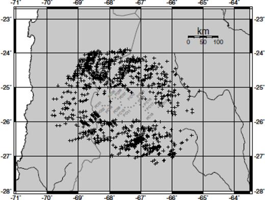
In this study, we use teleseismic data recorded along two E–W trending profiles across the Altiplano and Puna plateaus at 21°S and 25.5°S, respectively (Fig. 1). The topography of the Moho, the subducted slab and the upper-mantle discontinuities are investigated using P receiver functions. We analyse data of the ReFuCA project, a passive source experiment carried out in the framework of the collaborative research program ‘Deformation processes in the Andes’ (SFB-267). Instruments were set up in cooperation with GeoForschungsZentrum Potsdam and South American partners. The northern profile (hereafter referred to as RF profile) transects the Altiplano plateau along 21°S and extends the reflection line of the ANCORP'96 project (ANCORP Working Group 2003) about ∼200 km to the east. A total of 59 seismological stations were deployed from 2002 March to 2004 January between the coast of Chile (70°W) and the Bolivian Inter-Andean region (64.5°W). Nine stations were equipped with Guralp CMG-3ESP broad-band seismometers and SAM digitizers. Three stations consisted of CMG-40T seismometers with RefTek recorders. The other stations operated with short-period 1-Hz MARK L43-D seismometers using RefTek or EDL digital recorders. The length of the RF profile was ∼600 km and the station spacing was about 10 km.
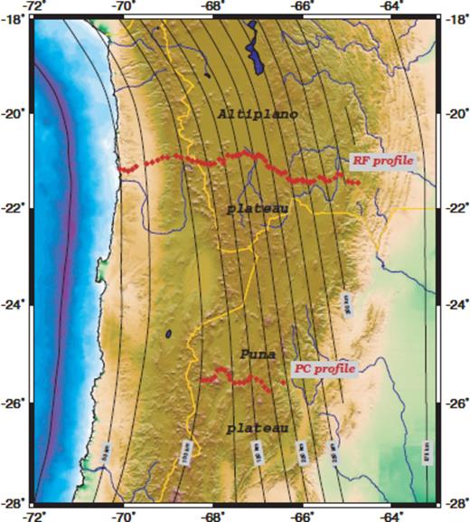
Map showing station locations (red diamonds) of the Altiplano profile (RF) and the Puna profile (PC) in the Central Andes. The black lines indicate depths to the WBZ (Cahill & Isacks 1992).
The southern profile (hereafter referred to as PC profile) is located in the Puna plateau between the volcanic arc to the west (68.5°W) and the Eastern Cordillera to the east (66.5°W). The profile consists of 19 stations: nine broadband and 10 short period. The profile was ∼200 km long and the stations were operational between 2002 July and 2004 January. On both profiles, PC and RF, data are recorded with sampling frequencies of 100 and 50 Hz, respectively.
We use selected teleseismic events with magnitudes ≥5.5mb at epicentral distances between 30° and 95° (Fig. 2) to examine P-to-S converted seismic phases. We apply the receiver function technique as described by Yuan et al. (1997): first, we resample all traces with 20 Hz. To make stations comparable, we restore the true ground motion by using a displacement restitution filter. Seismograms are then rotated into the ray coordinate system (L, Q, T) with the components oriented in the directions of the P-, SV- and SH-waves, respectively.
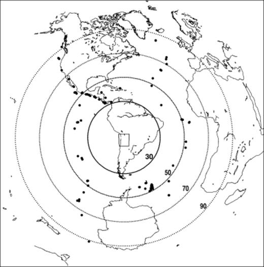
Distribution of teleseismic earthquakes used in this study. Events accumulate in the SE (Sandwich region) and in the NW (along the west coast of Central and North America), respectively. The circles denote the epicentral distance given in degrees.
To optimize the rotation process, we use the observed backazimuth and incident angles derived from the eigenvalues of the covariance matrix. We compare them with the theoretical rotation angles computed for the IASP91 reference earth model (Kennett & Engdahl 1991). If the difference exceeds 40° or 30° in back azimuth or incidence angle, respectively, theoretical angles are used for rotation to avoid false readings caused by noise influence. If the deviation of the incidence angle exceeds 50°, we remove the event from the data set. By deconvolving the P-waveforms on the L-component from the corresponding Q- and T-components, we remove the source and path effects. We obtain a total of 2499 receiver functions for the RF profile and 1659 for the PC profile, respectively.
As the amplitude of a converted phase is only a few per cent of the incident signal, we increase the signal-to-noise ratio by stacking the receiver function traces using two discriminative approaches. (1) The first is the binning procedure where single traces from different events and stations are stacked according to neighbouring piercing point locations at a given depth. Before stacking a moveout correction is applied to account for variations of delay times of converted phases relative to the originating P-wave with epicentral distance. We use a reference slowness of 6.4 s deg.−1, which corresponds to an epicentral distance of 67°. The summation enhances coherent signal whereas simultaneously suppressing random background noise. In the arc and backarc regions, strong attenuation has been suggested from Qp observations (e.g. Schurr et al. 2003, 2006). Therefore, we apply the sliding window technique, that is, binning windows slightly overlap. This leads to lateral smoothing and considerably improves the signal where the coverage is poor. (2) The second approach is the migration method (e.g. Kosarev et al. 1999; Kind et al. 2002). We use a back projection technique where incident ray paths are traced back according to a reference velocity model described in the next section. In this study, broader cones rather than rays have been back projected to account for increasing width of the Fresnel zones with depth.
3 Velocity Model
Using an inappropriate velocity model would result in false depth derived from migration, and would also influence the computation of piercing point locations. For this reason, the selection of the velocity model has strong impact. We start with a 1-D model derived from a joint inversion of velocity structures, station delays and hypocentre positions down to 230 km depth from Schurr et al. (1999). For deeper portions we use the global IASP91 reference model (Kennett & Engdahl 1991) assuming, that the processes of subduction, crustal thickening and plateau formation only affect the shallower parts of the upper mantle. Depths to Moho derived from this model fit reasonably well to the results of previous studies (e.g. Giese et al. 1999; Schurr et al. 1999; Yuan et al. 2000, 2002). However, in the migration section the major upper-mantle discontinuities at depths of 410 and 660 km, respectively, are imaged far too deep mainly due to the very high sublithospheric velocities of the inversion model in Schurr et al. (1999). Therefore, we modify the starting model by lowering the velocities beneath 125 km depth conforming more to the values of the IASP91 model. We also include a crustal low-velocity layer corresponding to the Altiplano low-velocity zone (ALVZ; Yuan et al. 2000) and a slight velocity decreases at 80 km depth corresponding to the lithosphere-asthenosphere boundary (hereafter referred to as LAB, Heit et al. 2007). The S wave velocity profiles are compared in Fig. 3.
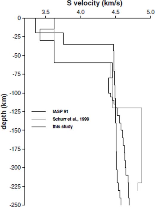
Comparison of S-wave velocity models. The thick black line marks the model used in this study. It is based on the inversion results of Schurr et al. (1999) marked by the grey line. We modify their model by adding a crustal low velocity layer (ALVZ) and a negative step corresponding to the lithosphere-asthenosphere boundary. Below a depth of 120 km, we use lower S-wave velocities than Schurr et al. to better fit the depths to the upper-mantle discontinuities obtained from the migration to global average values of 410 and 660 km, respectively. The thin black line denotes the global reference model IASP91 (Kennett & Engdahl 1991).
4 Observations and Discussion
In general, the observations are limited to a high-frequency band due to the short-period instrument responses. In some cases, even after restitution, the signal decreases at periods falling below 6 s. The frequency content is also depending on the station locations and points to attenuation variations. In the forearc, Qp values are uniformly high in contrast to those in the backarc region where low Qp values are attributed to fluids and elevated temperatures. Attenuation significantly alters the recorded waveforms and, in some parts, even leads to a complete lack of S wave energy (Schurr et al. 2003, 2006).
We observe similar changes in our receiver function data illustrated by means of single receiver functions of the MW 7.6 event on 2003 August 4 (Fig. 4). Traces are obtained from broad-band station RF48 (bottom) and from short-period stations RF59 (middle) and RF09 (top). RF48 and RF59 are located in the backarc region in the easternmost part of the Altiplano profile. The short-period station RF59 is not able to detect the long periods prevailing at the broad-band station. However, both traces display a rather low frequency waveform compared to the forearc station RF09, which is clearly dominated by higher frequencies.
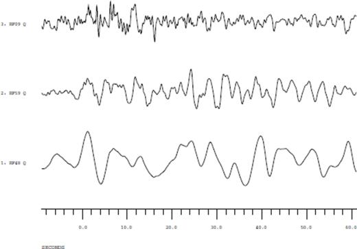
Data example for the 2003 August 4 event. The traces show final receiver functions computed from records of broad-band station RF48 (bottom) and of two short period stations, one of which located in the back arc (RF59, middle) and the other one placed in the fore arc region (RF09, top). A 5 Hz lowpass filter is applied to avoid aliasing effects caused by resampling. Comparison of the waveforms demonstrates the different frequency contents. As the PC profile is much shorter, we only show stations from the RF profile.
4.1 Altiplano plateau
The RF profile is in particular affected by a limited frequency content caused by attenuation and a rather high noise level. Due to the resulting lack of long-period signal the detection of broad gradual velocity transitions is difficult. We do not obtain a clear signal from the mantle transition zone underneath the Altiplano plateau. In Fig. 5, we present the binning section along the RF profile in the time domain. Before stacking, traces are filtered with a 3 Hz to 5 s bandpass and sorted from west to east by piercing points at a depth of 70 km (Moho depth from Yuan et al. 2000) with a corresponding delay time relative to P onset of 8.84 s. Resolution is usually estimated from the first Fresnel zones. Here, the dominating period is about 2.5 s. We compute λ/4-Fresnel zones for a single ray of roughly 16.6 and 23.7 km at depths of 60 and 100 km, respectively. However, effectively, the resolution is much better due to overlapping Fresnel zones and dense ray coverage. We select a small binning width of approx. 3 km to most efficiently stack coherent signal originating at dipping structures. Lateral smoothing is obtained from bins overlapping by ca. 1 km. The associated depth migrated section is displayed in Fig. 6. Here, we use a 3 Hz to 8 s bandpass filter before applying the method described above. We include hypocentre locations from Engdahl et al. (1998) between 20°S and 22°S.
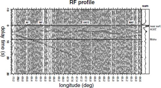
Section of binned traces along the RF profile using 3 Hz to 5 s bandpass filter. Traces are sorted by piercing points calculated for a depth of 70 km using the velocity model shown in Fig. 3. The labels at zero time denote fault systems occurring at the surface: AF – Atacama Fault, WF – West Fissure, UKFZ – Uyuni Kenayani Fault Zone and MAT – Main Andean Thrust. The thin solid line marks the corresponding delay time of 8.84 s. We select a binning width of 0.03° with 0.01° overlapping. The Moho converted phase (dashed line) appears very weak and becomes seismically invisible at about 66.8°W. The dipping slab is clearly mapped to 12 s delay time and can be traced further down to ca. 19 s (dashed line, left-hand side). Within the crust, we see a pronounced negative arrival ranging from 1–3 s followed by a weaker positive phase, which we both relate to the ALVZ. Finally, a relatively shallow dipping interface is found in the westernmost part of the profile. Crustal converted phases are marked with dotted lines.
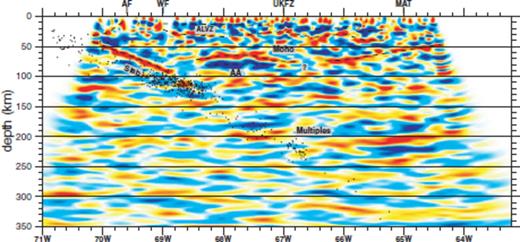
Migrated section to 350 km depth along the RF profile using a 3 Hz to 8 s bandpass filter. The dashed lines mark the structures also recognized in the binning section (Fig. 5). The black dots indicate hypocentre locations between latitudes of 20–22°S (Engdahl et al. 1998). The east-dipping slab converted phase stands out clearly down to roughly 120 km. The signal originating at the Moho is more pronounced than in the stacked traces, but still exhibits a gap between 67.0–66.5°W. The same crustal structures are identified as denoted in Fig. 5. In addition, a strong negative asthenospheric anomaly (labelled as AA) occurs beneath the deflected Moho segment between 68.3 and 67.1°W.
High-amplitude converted phases originating near the surface stretch across the entire binning section (Fig. 5). These are most likely related to sediments covering the bedrock and are also seen in previous studies (e.g. Yuan et al. 2000, 2002). Besides the shallow sediments, we identify four pronounced features in both figures as discussed below: The Nazca slab, the continental Moho, an intracrustal low velocity layer (ALVZ) and a dipping structure within the western part of the crust.
(1) Slab: strong positive signal occurs in the westernmost part of the profile (left-hand side) being generated at the inclined structure of the subducting plate. The amplitude is strong in the shallower western part until reaching a delay time of roughly 13 s corresponding to a depth of about 110 km at 68.8°W (Fig. 5). Though amplitudes are weak, the coherent signal can be traced further to delay times of 20 s (175 km) at 67.4°W. However, it has to be considered, that sorting of the traces is only appropriate at 8.86 s indicated by the thin line. The termination of the high-amplitude conversions can also clearly be identified in Fig. 6. Lateral smearing occurs due to the overlapping bins. Thus, weak phases generated at non-horizontal interfaces are annihilated, especially at greater depths where Fresnel zones increase in width. It has to be mentioned that the depth and the dip of inclined structures are not properly imaged with the customary migration method. To improve detection of the slab signal, we adopt a technique accounting for dipping interfaces as applied by Li et al. (2000). The resulting section exhibits only minor changes pertaining to the inclination but does not influence the general findings and is not presented here.
The positive polarization (dark and red signals in Figs 5 and 6, respectively) denotes an upward velocity decrease, which we explain as the Moho discontinuity of the downgoing slab. The fading slab-signal at roughly 110 km is caused by reduced impedance contrast. This is within the expected depth range for the completion of eclogitization of oceanic gabbro. This transformation involves release of water, which enhances rock failure and may thus trigger seismicity (e.g. Bock et al. 2000; Yuan et al. 2000; Abers et al. 2006). The occurrence of dehydration embrittlement is confirmed in Fig. 6 by the correlation of increased seismicity and the weakening of the slab converted phase.
(2) Continental Moho: in the binning section (Fig. 5), the signal from the continental Moho is uncommonly weak and reveals a gap at about 66.8°W. The weakness of the Moho conversion indicates a gradual velocity change from the crust to the mantle rather than a sharp boundary. This approves the interpretation from seismic reflection data, where no Moho signal has been observed (ANCORP working group 2003). The signal is more distinctive in the migrated section, but the gap still remains. To the east of the gap, the Moho is continuously shallowing from ca. 80 (∼9.9 s) to 45 km (∼6.0 s). This shallowing coincides with the subsequent occurrence of a high velocity block found by teleseismic tomography (Heit 2005; Heit et al. 2008) and has been interpreted as the Brazilian Shield, which seems not to be affected by crustal shortening. To the west of the gap, the converted signal is strongest between 67°W and 69°W revealing a slight upward deflection. Delay times between 8 and 9 s indicate a mean depth to Moho of about 70 km, which is also visible in the migration results (Fig. 6) and agrees well with previous results (e.g. Beck et al. 1996). Further to the west, beyond 69°W, no clear signal from the Moho is detected.
A strong negative anomaly is detected directly beneath the deflected part of the continental Moho between 68.3°W and 67.1°W at 80 km depth, which is most obvious in Fig. 6 but also slightly present in Fig. 5. The negative phase marks a layer exhibiting strongly decreased velocities that appears at the same position where a low velocity anomaly is independently derived from the same data set applying the teleseismic tomography method (Heit et al. 2008). A previous receiver function study (Yuan et al. 2000) did not detect this anomaly as should have been expected due to the strong amplitude revealed in this study. However, the investigated areas do not directly cover the same latitude range. Therefore, the presence of a rather local low velocity zone could add some evidence to a possible scenario of lithospheric delamination of local extent, which is one of the models discussed in the context of high uplift rates of the Altiplano (Garzione et al. 2006). The removal of a lithospheric block as suggested by Heit et al. (2008) would help the ascension of hot asthenospheric material filling in the gap from the delaminated portion of the lithosphere producing as a result a layer with anomalous low velocities at the base of the crust.
(3) Low velocity layer: a wide-spread low-velocity layer correlating with the ALVZ can be clearly seen in the binning section in Fig. 5 (subhorizontal dotted lines). The top of the layer appears as a pronounced negative phase with delay times ranging from 1.5 to 2.5 s according to a mean depth of about 16 km. It is followed by a positive signal 1–3 s later marking the lower boundary. On average, we derive a layer thickness of about 15 km in agreement with previous results (e.g. Yuan et al. 2000; ANCORP Working Group 2003). The frequency range used in this study allows for high vertical resolution of about 2.25 km allowing to detect strong topography of the lower bound of the low-velocity layer. Topography, again, reduces the distinctness of both the upper and lower boundary in the migrated section (Fig. 6).
We repeat the stacking procedure with piercing points computed for a depth of 20 km (Fig. 7) to avoid false sorting of the traces. The lower boundary appears a little more pronounced but remains more diffuse than the top of the layer. To the west, the lower boundary of the ALVZ terminates at 68.8°W correlating well with the position of the Quebrada Blanca Bright Spot (QBBS). The QBBS is a strong reflection anomaly that has been detected by a steep angle seismic experiment (ANCORP Working Group 1999 & 2003; Yoon et al. 2003) and has been linked to the presence of fluids released from the subducting slab. This suggestion has become more evident in local tomographic images obtained by Koulakov et al. (2006). By observing the binning section in Fig. 7, it is possible to suggest a correlation between the ALVZ and the QBBS as both are located at nearly the same depth and have the aspect of a low-velocity unit. The upper boundary of this low-velocity layer is interrupted at 69.0°W (also seen in Fig. 6) and can be traced at slightly shallower depths near 69.6°W. The position of the gap coincides with the West Fissure fault system, which is believed to be a vertical fault zone also reaching down to the depths of the QBBS (e.g. ANCORP Working Group 2003; Heit et al. 2008).
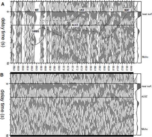
(A) Binned section as described in Fig. 5 but focusing on shallower structures. Piercing points are calculated for 20 km depth corresponding to a delay time of 2.6 s (solid line). Upper and lower ALVZ boundaries are denoted by dashed lines. The segmentation of the upper bound coincides with the dipping structures (dotted lines) and in two cases correlate with the UKF and MAT lineaments at the surface. For the other one at approximately 65.8°W, no surface structure has been reported so far. The signal originating at the QBBS, though not very well resolved, can be imaged at 69.0°W indicating a connection to the lower ALVZ boundary. (B) The same binned traces without markings. The distances of traces are not to scale to emphasise the coherency of the phases.
In the eastern part, the top of the ALVZ (Fig. 7) appears to be segmented by westward dipping faults between 67°W and 66°W. The segmentation is associated with vertical offsets of some 8–10 km where as the bottom is more continuous, also revealing depth variations. The ALVZ terminates between 65.6°W and 65.4°W where the westward dipping main Andean thrust (MAT) is located. The first step in the upper boundary at 67°W is concordant with the location of the Uyuni-Kenayani Fault Zone (UKFZ). Yet, neither of both structures (i.e. MAT and UKFZ) can be convincingly corroborated by the presence of clear converted phases, where as weak signal occurs at the second step near 65.8°W. This feature is vaguely observable in Fig. 5 and confirmed by making use of piercing points at shallower depth in Fig. 7. However, no related fault is known at this position on the surface and the evidence arising from Figs 5 and 7 is only faint. From the segmentation of the upper boundary and correlating positions, we indirectly presume that the major fault systems extend into the ALVZ, that is, down to depths of about 15 km but do not penetrate into the lower crust. Our analysis supports the interpretation of the ALVZ being a weak partial-melt layer, which could serve as an intracrustal detachment zone as it is required by the simple shear model (e.g. Allmendinger & Gubbels 1996; Babeyko & Sobolev 2005).
(4) Dipping interface: we detect a further inclined upper crustal structure at the westernmost part of the profile. The interface is dipping to the west from near surface at 69.6°W and can be traced in Fig. 5 down to delay times of ca. 4 s, that is, 30 km, at 70.2°W where it approaches the Nazca slab. The nature of this interface is unclear. It seems to reach the surface at the position of the Atacama Fault (AF), which has been described as a subvertical to slightly east-dipping normal fault (e.g. Delouis et al. 1998) that extends about 1000 km along the coastal ranges of northern Chile. However, it is possible that the west dipping interface detected in this study might be related to the location of the AF at the surface as well as to a zone of Jurassic underplating at depth assumed from reflection data (ANCORP Working Group 2003). A relationship between both structures has not yet been observed possibly due to a gradual velocity transition within the fracture zone that cannot be detected at higher frequencies.
4.2 Puna plateau
The PC profile is much shorter than the RF profile and is limited to the Puna plateau. The depth to the slab derived from the Wadati–Benioff zone (WBZ; Cahill & Isacks 1992) ranges between 100 and 200 km from west to east (Fig. 1). At that depth, the gabbro-eclogite transition should already be completed, so the slab is expected to be more or less invisible for receiver functions. To image the crustal structure, we apply the same processing steps and filters as described in 4.1. We slightly change the binning parameters using a binning width of 0.025° with an overlap of 0.005°. For the Puna profile, we calculate piercing points for a depth of 60 km equivalent to the expected Moho depth below this area (Schurr et al. 1999). A second binning section with shallower piercing points (25 km) is computed to consider different order of traces at different depths. The resulting sections are presented in Figs 8(a) and (b). The comparative migration method described above is used for lithospheric depths without alteration and its result is illustrated in Fig. 9. We include hypocentre locations computed by Engdahl et al. (1998) with latitudes ranging between 24 and 26°S.
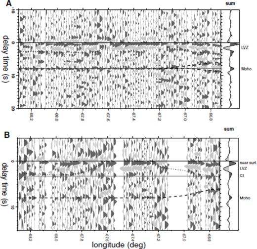
Section of stacked traces along the PC profile using a 3 Hz to 5 s bandpass filter similar to Fig. 5. In Section A, traces are sorted by piercing points computed for 60 km depth and binned in steps of 0.025° with a slight overlap of 0.005°. To investigate the shallow crustal structures, in Section B, we sort traces by piercing points calculated for a depth of 25 km. Here, a binning width of 0.015° is used, again with 0.005° overlapping. In both sections, the dashed lines mark the Moho converted phase. In Section A, the Moho phase, apparently, splits up in the eastern part whereas in Section B only the shallowing branch is confirmed. The dotted lines mark dipping interfaces at shallow depths within the crust referred to as CI (crustal interfaces).
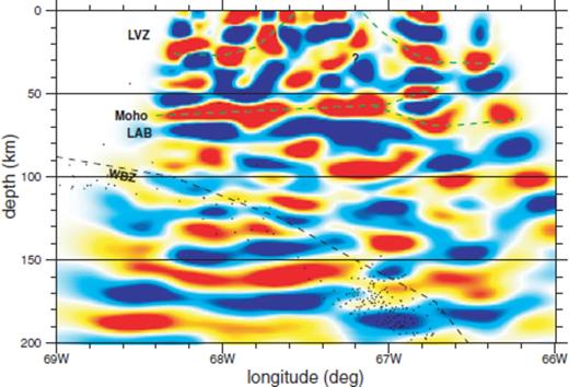
Migrated section of the crust and uppermost mantle along the PC profile. A bandpass filter from 3 Hz to 8 s is applied. The black line denotes the depth to the middle of the WBZ derived by Cahill & Isacks (1992), black dots mark the hypocentre positions between 24°S and 26°S located by Engdahl et al. (1998). Green lines emphasise the observed structures confirming those in the binning section. Additionally, a westward dipping crustal interface appears between 67 and 68°W, but, much less striking in Fig. 8 probably being an artefact.
The stacked traces displayed in Fig. 8 show converted phases much more pronounced than those obtained from the RF profile (Fig. 5). Immediately after the P-onset a dominating near-surface conversion is detected. The noise level is lower than for the RF profile and the crustal structure is less disguised exhibiting similar features as observed in the Altiplano. The continental Moho is clearly imaged, as well as a pronounced negative signal at 1–2 s delay time. Two dipping interfaces can be recognized in the upper half of the crust. The associated migrated section (Fig. 9) presents similar features in general but differs slightly in detail. In both sections, the slab converted phase is absent. Finally, we present a migrated section at longer periods (Fig. 10) down to 800 km illuminating the mantle transition zone.
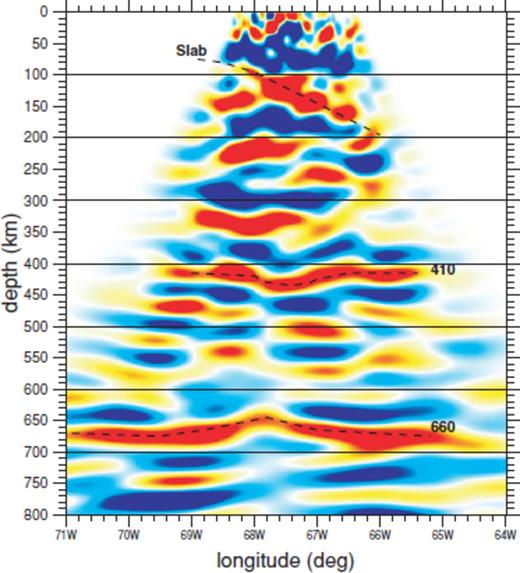
Migrated deep section along the PC profile. We apply a bandpass filter from 5 to 20 s. Lithospheric structures cannot be resolved in this frequency band, where as we observe a distinct slab signal. Converted phases originating at the major upper-mantle discontinuities at 410 and 660 km depth reveal anomalous down- and upwelling, respectively. Based on the Clapeyron-slopes of the underlying mineral phase transitions, the anomalies are typical for locally increased temperature in the mantle.
(1) Moho: we map the Moho as a plane interface at 7.8 s delay time corresponding to the expected depth of roughly 60 km without significant topography between 68.6 and 67.1°W. Further to the east, in Figs 8(a) and 9, the Moho signal apparently bifurcates with one branch shallowing to depths of 47 km at 66.7°W. The second branch is dipping downward reaching nearly 70 km depth. The latter phase is more pronounced in the migrated section (Fig. 9) but with lower resolution. We interpret the deeper branch as an artefact, most likely caused by multiple reflections generated at the crustal interfaces. This consideration is supported by Fig. 8(b) where piercing points at 25 km depth are used for sorting. Here, only the shallower interface remains.
Similar to the Altiplano, the Moho signal is rather weak beneath the Puna although less disturbed. At longer periods (Fig. 9), the Moho phase is immediately followed by distinct negative signal in the western part (67°W), where also the multiple signal interferes. A similar negative anomaly appears beneath the Altiplano (e.g. in Fig. 6) roughly at the same longitude range. The negative signal must emerge from a downward velocity decrease and is most likely related to hot asthenospheric material situated underneath the crust (referred to as LAB). The anomaly could be related to the loss of a lithospheric root on a broad scale as suggested by the delamination model for the Central Andes (e.g. Kay & Kay 1993; Schurr et al. 2006).
(2) LVZ and crustal interfaces: a pronounced negative signal is also detected within the crust, best imaged in the binning section in Fig. 8(b) at nearly constant delay times of 1.65 s (13 km depth). This is in fair agreement with the top of the ALVZ verified underneath the RF profile and we therefore assume that the low-velocity layer extends to the PC profile, as can also be derived from Yuan et al. 2000. The negative anomaly is dissected by two dipping interfaces. To the west of 67.7°W, the signal is still present, but weaker than in the other parts. Unlike the northern RF profile, the segmentation along the PC profile does not lead to vertical shifts of the discontinuities and the negative phases remain at constant delay times. The migrated section (Fig. 9) indicates a further structure within the crust dipping to the west. We do not interpret this signal, as it is not confirmed by the binning sections.
The first intersecting interface is dipping to the west from 67.6°W at the surface and merges at 67.9°W into a subhorizontal positive structure located at about 21 km (∼2.7 s). From the data, we cannot distinguish whether this structure is simply continuing at constant depth or if it only terminates at the contact with the horizontal interface. It possibly marks the lower boundary of the LVZ, but we are not able to detect a continuous interface clearly related to it.
(3) Slab: as a result of eclogitization, the signal originating from the slab becomes very weak. Therefore, the slab cannot be detected in the binning section (Fig. 8). In the migrated section (Fig. 9), the theoretical depths of the WBZ is shown derived from hypocentres (black dots) of neighbour event locations (Cahill & Isacks 1992). Very weak signal occurs 10–20 km above the WBZ, which may be suggestive of the slab conversion. The misfit of the dip angle could be explained be the migration process and can be corrected using the dip migration technique (Li et al. 2000). However, no evidence can be derived from the data due to the weakness of the signal. A stronger converted phase occurs at the same depth range when we use longer periods as further described below (Fig. 10).
(4) Mantle transition zone:Fig. 10 displays a migrated section down to 800 km depths beneath the PC profile. We apply a bandpass filter from 5 to 20 s to better image the major discontinuities of the mantle transition zone at 410 and 660 km depth (referred to as ‘410’ and ‘660’, respectively). Whereas the long-period signal is suitable to detect velocity gradient zones, the small-scale crustal structure is not resolved here. The upper part of the section is dominated by a smeared negative phase, which we relate to the LAB and is also seen by Heit et al. (2007). It is followed by an eastwards dipping interface, which can be traced down to 200 km at 66°W. We interpret this interface as the subducting slab. Both upper-mantle discontinuities can be clearly identified roughly at the expected depths. However, the velocity model introduced in Section 3 has been constructed particularly to better fit the shallower lithospheric structures and does not reliably reflect the deeper velocity structure. We thus focus on differential traveltimes of both mantle discontinuities.
In general, the 410 and 660 equally appear about 10 km deeper than the global average, so their differential traveltime still agrees well to IASP91. Surprisingly, both, the 410 and 660 discontinuities reveal significant depth anomalies at the central part of the profile between 67.5°W and 68°W. The 660 seems to be upwardly deflected by 20 km, where as the 410 exhibits a downwelling of 15–20 km. It is well known, that the mantle discontinuities seismically reflect mineral phase transitions in the olivine system, reversely dependent on pressure and temperature (e.g. Bina & Helffrich 1994). The downwelling of the 410 and the simultaneous upwelling of the 660, as observed here, could be explained by an increase in temperature, which may be possibly caused by a rising mantle plume.
The thinning of the mantle transition zone by about 40 km (Fig. 10) corresponds to approximately 300 K excess temperature (Collins et al. 2002). However, it is important to mention that the ray coverage is rather poor in the central part of the profile especially where the anomalies have been found. Fig. 11 shows the distribution of piercing points at a depth of 410 km. Nevertheless, from the opposite sign of the depth variations, we exclude the possibility of inappropriate velocities in our model, which would be capable of generating processing artefacts (i.e. ‘smileys’), as this effect would cause both interfaces to be deflected to the same direction. The projection of broad Fresnel zones used in the applied migration technique entails smearing effects annihilating the small-scale topography of the discontinuities. Moreover, the gap in ray coverage beneath the profile is partly reduced by the Fresnel zones. The smaller cut-off period of 5 s is taken as a basis to calculate λ/4-Fresnel zones (70 km at a depth of 410 km). As a consequence of the poor coverage at that depth, we do not determine any radius of the hypothesized plume-like structure. For the same reason, the derived thinning of about 40 km can only provide a rough estimate.
Distribution of piercing points calculated for a depth of 410 km. Converted phases generated at the mantle discontinuities have to be interpreted carefully, due to the lack of information directly beneath the profile.
5 Conclusions
Seismic data recorded at two dense profiles transecting the Altiplano and Puna plateaus in the Central Andes have been investigated with the P receiver function method. In general, the results evidence similar structures beneath both plateaus, but also exhibit some local differences. A crustal low-velocity layer (ALVZ) with its top boundary at about 15 km depth has been detected beneath both plateaus confirming previous results that interpret this as a layer of partially molten material (e.g. Yuan et al. 2000). From a high-resolution binning section beneath the Altiplano, we determine the thickness of the ALVZ to be 20 km. Whereas beneath the Puna no clear lower boundary has been found, indicating a rather diffuse transition to the lower crust at this area. We have detected several dipping interfaces cutting through the top of the ALVZ at both profiles. Beneath the RF profile, the interfaces are possibly related to the presence of some major faults known at the surface. The segmented top of the ALVZ demonstrates offsets in depth. Thus, it might act as a detachment zone within the crust as it would be required by the simple shear model (Babeyko & Sobolev 2005). Beneath the Puna plateau, we do neither see related fault zones at the surface nor significant offsets in the ALVZ upper bound. Here, the interfaces most likely mark velocity contrasts of hot fluid accumulations supplying the local Antofalla and Galan volcanoes as derived from a complementary tomographic study (Heit 2005).
An average crustal thickness of 70 km is observed beneath the Altiplano plateau. Anomalous thinning of the crust occurs in the central region. This upwardly deflected part of the Moho is followed by a negative anomaly. Beneath the Puna, the crust is about 10 km thinner but shows no irregular topography. The LAB beneath the Puna plateau can be traced along the entire profile roughly spanning the same longitude range as the negative anomaly at the Altiplano. The strong amplitude of the negative signal indicates a significant S-velocity decrease most likely associated to partially molten material. Beneath the Altiplano, we find this anomaly to be locally confined to the area beneath the volcanic arc and further east, so reduced velocities could be related to melt accumulations below the crust. However, this would not explain the anomalous thinning of the overlying crust as indicated by the deflected Moho signal. A possible mechanism would be the local delamination of the lithosphere including parts of the lowermost crust. Excess temperature and enhanced melt generation would be the result of ascending hot asthenosphere replacing the delaminated block. Due to the limited length of the PC profile, we are unable to determine the lateral extent of the analogous negative anomaly beneath the Puna plateau. The amplitudes, again, indicate strongly reduced velocities similar to the RF profile. Taking into consideration that the crust is thinner by some 10 km, removal of lower crust to a greater extent than below the Altiplano plateau would be possible.
Converted phases generated at the slab interface fade at roughly 110 km below the RF profile coinciding with the expected completion depth of the gabbro-eclogite transition. The signal can be traced only weakly down to 160 km depth. Beneath the PC profile, the slab is only sampled at depths below 90 km and is virtually not detected at high frequencies. Unexpectedly, the slab can be imaged down to depths of about 200 km at longer periods. Findings from the tomographic study by Heit (2005) complement with low-velocity anomalies situated underneath the Antofalla and Galan volcanoes with an additional source of fluids released from the slab beneath Puna at roughly 200 km, which is deeper than commonly expected. The observed features reflect processes indicative for higher temperatures and enhanced heat flow in that region.
A possible reason has been derived from the deep cross-section imaging the major mantle discontinuities. Here, local thinning of the transition zone has been observed as it would be characteristic for a rising mantle plume. We have to point out, that the data coverage is poor particularly in the area where the anomaly is located, so reliability of this observation remains to be confirmed by future studies. For the same reason, we do not determine excess temperature and radius of this hypothetical plume. However, from the opposite signs of the deflections of the 410 and the 660, we rule out that these anomalies are only processing artefacts. Therefore, a mantle plume could be responsible for the increased heat flow and additional fluid release underneath the Puna plateau.
Acknowledgments
The ReFuCA project was funded by Deutsche Forschungsgemeinschaft (DFG Bonn) within the Collaborative Research Center 267 (SFB-267 Deformation Processes in the Andes). We would like to thank W. Hanka and staff from the GEOFON data centre and the Geophysical Instrument Pool Potsdam (GIPP) for providing instrumentation and equipment. For data processing, we have used the SeismicHandler software package (Stammler 1993). The figures have been generated using Generic Mapping Tools (Wessel & Smith 1998). We also thank two anonymous reviewers for their comments that helped to improve the manuscript.
References
